Many new variable stars discovered in the core of the globular cluster NGC 6715 (M54) with EMCCD observations

Abstract

Context. We show the benefits of using Electron-Multiplying CCDs and the shift-and-add technique as a tool to minimise the effects of the atmospheric turbulence such as blending between stars in crowded fields and to avoid saturated stars in the fields observed. We intend to complete, or improve, the census of the variable star population in globular cluster NGC 6715.

Aims. Our aim is to obtain high-precision time-series photometry of the very crowded central region of this stellar system via the collection of better angular resolution images than has been previously achieved with conventional CCDs on ground-based telescopes.

Methods. Observations were carried out using the Danish 1.54-m Telescope at the ESO La Silla observatory in Chile. The telescope is equipped with an Electron-Multiplying CCD that allowed to obtain short-exposure-time images (ten images per second) that were stacked using the shift-and-add technique to produce the normal-exposure-time images (minutes). The high precision photometry was performed via difference image analysis employing the DanDIA pipeline. We attempted automatic detection of variable stars in the field.

Results. We statistically analysed the light curves of 1405 stars in the crowded central region of NGC 6715 to automatically identify the variable stars present in this cluster. We found light curves for 17 previously known variable stars near the edges of our reference image (16 RR Lyrae and 1 semi-regular) and we discovered 67 new variables (30 RR Lyrae, 21 long-period irregular, 3 semi-regular, 1 W Virginis, 1 eclipsing binary, and 11 unclassified). Photometric measurements for these stars are available in electronic form through the Strasbourg Astronomical Data Centre.

1 Introduction

Galactic globular clusters are interesting stellar systems in Astronomy as they are fossils of the early Galaxy formation and evolution. This makes them excellent laboratories in a wide range of topics from Stellar Evolution to Cosmology, from observations to theory.

NGC 6715 (M54) was discovered on July 24, 1778 by Charles Messier. The cluster is in the Sagittarius Dwarf Spheroidal galaxy at a distance of 26.5 kpc from our Sun and 18.9 kpc from our Galactic centre. It has a metallicity [Fe/H]=$-$1.49 dex and a distance modulus (m$-$M)_V=17.58 mag. The magnitude of its horizontal branch is V_HB=18.16 mag (2010 version Harris, 1996). The stellar population and morphology of NGC 6715 have attracted the attention of several studies. Although NGC 6715’s position is aligned with the central region of the Sagittarius Dwarf Spheroidal galaxy, recent studies have shown that this cluster is not the nucleus of the mentioned galaxy (Layden & Sarajedini, 2000; Majewski et al., 2003; Monaco et al., 2005; Bellazzini et al., 2008). Carretta et al. (2010) found that the metallicity spread in this cluster is intermediate between smaller-normal Galactic globular clusters and metallicity values associated with dwarf galaxies. It has a very peculiar colour-magnitude diagram with multiple main sequences, turnoff points and an extended blue horizontal branch (HB) (Siegel et al., 2007; Milone, 2015). Rosenberg et al. (2004) found that this cluster hosts a blue hook stellar population in its blue HB. It is thought that NGC 6715 might host an intermediate mass black hole (IMBH) in its centre (Ibata et al., 2009; Wrobel et al., 2011) as well.

Oosterhoff (1939) found that globular clusters can be classified into two groups based on the mean periods and the number ratios of their RR0 and RR1 stars. These are the Oosterhoff I (OoI) and Oosterhoff II (OoII) groups, and this is known as the Oosterhoff dichotomy. It was also found that the metallicity of the clusters plays an important role in this classification (Kinman, 1959) and that it could be related with the formation history of the Galactic halo (see e. g. discussions in Lee & Carney, 1999; Catelan, 2004, 2009; Smith et al., 2011; Sollima et al., 2014).

The first Oosterhoff classification for NGC 6715 was done by Layden & Sarajedini (2000) by comparing the amplitudes and periods of 67 RR Lyrae in this cluster with the period-amplitude relation obtained for M3 (OoI) and M9 (OoII). NGC 6715 follows the relation defined by M3 and this implies that it is an OoI cluster. They also found that the mean periods of the RR Lyrae also agree with the OoI classification. Similarly, Sollima et al. (2010) in their study of variable stars in NGC 6715 discovered a new set of 80 RR Lyrae, and they used 95 RR0 and 33 RR1 (after excluding non-members or problematic stars) to find that this cluster shares some properties of both OoI and OoII clusters. For instance, the average period of its RR0 and RR1 stars was found to be intermediate between the values for the OoI and OoII classifications. We note that Catelan (2009) also classified this cluster as an intermediate Oosterhoff type based on its position in the $<P_{\mathrm{RR0}}>$-metallicity diagram.

Several time-series photometric studies focused on the variable star population (Rosino, 1952; Rosino & Nobili, 1958; Layden & Sarajedini, 2000; Sollima et al., 2010; Li & Qian, 2013), but due to the high concentration of stars in its core, many variables have previously been missed due to blending. NGC 6715 is very massive and it is among the densest known globular clusters (Pryor & Meylan, 1993). Due to this, NGC 6715 also took our attention as an excellent candidate for our study of globular clusters using Electron-Multiplying CCDs (EMCCDs) and the shift-and-add technique (Skottfelt et al., 2013, 2015a; Figuera Jaimes et al., 2016).

Section 2 summarises the observations, the reduction, and photometric techniques employed. Section 3 explains the calibration applied to the instrumental magnitudes. Section 4 contains the technique used in the detection and extraction of variable stars. Sections 5 and 6 show the methodology used to classify variables and the color-magnitude diagrams employed, respectively. Section 7 presents our results and Section 8 discusses the Oosterhoff classification of this cluster. Our conclusions are presented in 9.

2 Data, reduction, and photometry

EMCCDs, also known as low light level charge-coupled devices (L3CCD) (see e. g. Smith et al., 2008; Jerram et al., 2001), are conventional CCDs that have an extended readout register where the signal is amplified by impact ionisation before they are read out. Hence the readout noise is negligible when compared to the signal and very high frame-rates become feasible (10-100 frames/s). This provides an opportunity to compensate for the blurring effect of the turbulence in the atmosphere. By shifting and adding the individual frames appropriately, it is possible to construct much higher resolution images than is possible using conventional CCD imaging from the ground. Furthermore, the dynamic range of the stacked images is greatly increased and the saturation of bright stars is therefore not an issue except for the very brightest stars in the sky. However, the main drawback with this technique is that the process whereby the signal is amplified also increases the photon noise component in the images by a factor of $\sqrt{2}$ when compared to conventinal CCD images. One should also be aware that EMCCD imaging data need to be calibrated in a different way to conventional CCD data. Several studies where EMCCDs have been used can be found in the literature e.g. high-resolution imaging of exoplanet host stars in the search for unseen companions (Southworth et al., 2015; Ciceri et al., 2016; Bozza et al., 2016; Street et al., 2016; Evans et al., 2016) photometric and astrometric measurements of a pair of very close brown dwarfs (Mancini et al., 2015), and time-series photometry of crowded globular cluster cores aiming to complete the census of variable stars (Skottfelt et al., 2015a; Figuera Jaimes et al., 2016).

The data presented in this paper are the result of EMCCD observations performed over three consecutive years: 2013, 2014 and 2015 in April to September each year. The 1.54 m Danish telescope at the ESO Observatory in La Silla, Chile was used with an Andor Technology iXon+897 EMCCD camera, which has a 512 $\times$ 512 array of 16 $\mu$m pixels, giving a pixel scale of $\sim 0^{\prime\prime}$.09 per pixel and a total field of view of $\sim 45\times 45$ arcsec².

For this research the EMCCD camera was set to work at a frame-rate of 10 Hz (ten frames per second) and an EM gain of $300e^{-}$/photon. The camera was placed behind a dichroic mirror which works as a long-pass filter. Taking the mirror and the sensitivity of the camera into consideration, it is possible to cover the wavelength range from 650 nm to 1050 nm. This is roughly a combination of SDSS $\mathrm{i}^{\prime}+\mathrm{z}^{\prime}$ filters (Bessell, 2005). More details about the instrument can be found in Skottfelt et al. (2015b). The total exposure time employed for a single observation was 10 minutes, which means that each observation is the result of shifting-and-adding 6000 exposures. The resulting PSF FWHM in the reference image employed in the photometric reductions (see below) was 0.44^′′.

In Figure 1, histograms of the number of observations per night during each year are shown. Data in the left-hand panel correspond to 2013, data in the middle panel to 2014 and data in the right-hand panel to 2015. We aimed to always take two observations per night, although it was not always possible due to weather conditions or time slots needed for other projects as is the case of the monitoring of microlensing events carried out by the MiNDSTEp consortium.

Figure 1: Histograms with the number of observations per night for globular cluster NGC 6715. Left: 2013. Middle 2014. Right: 2015.

Bias, flat-field and tip-tilt corrections, were performed using the procedures and algorithms described in Harpsøe et al. (2012). In particular, the tip-tilt correction allows high-resolution stacked images to be created as described in detail in Skottfelt et al. (2015a); Figuera Jaimes et al. (2016). Briefly, the method uses the Fourier cross correlation theorem where, for each bias- and flat-corrected exposure $I_{k}(i,j)$ within an observation, we calculate the cross correlation image between $I_{k}(i,j)$ and an average of 100 randomly chosen exposures. The peak in the cross correlation image gives the appropriate shift to correct the tip-tilt error. We then stack the shifted exposures according to batches grouped by image quality (a measure of image sharpness), to create ten-layer image cubes. The best quality layers from each cube (i.e. the sharpest layers) are extracted from all of the available observations to create a high-resolution reference image for subsequent difference image analysis (DIA). Finally, each ten-layer cube is stacked to create a single image corresponding to each observation.

To extract the photometry in each of the stacked images we used the DanDIA pipeline (Bramich, 2008; Bramich et al., 2013), which is based on difference image analysis (DIA; Alard & Lupton, 1998; Alard, 2000). The pipeline works by aligning all images to the reference image, solving for a set of convolution kernels modelled as discrete pixel arrays, and subtracting the convolved reference image in each case to create a set of difference images. Stars are detected on the reference image and their reference fluxes $f_{\mathrm{ref}}$ (ADU/s) are measured using PSF photometry. Difference fluxes $f_{\mathrm{diff}}(t)$ (ADU/s) for each star detected in the reference image are measured in each of the difference images by optimally scaling the PSF model for the star to the difference image. The light curve for each star in instrumental magnitudes $m_{\mathrm{ins}}$ are built as shown in Eqn. (1)

$$m_{\mathrm{ins}}(t)=17.5-2.5\log(f_{\mathrm{tot}}(t)),$$ (1)

where $f_{\mathrm{tot}}(t)$ is the total flux in ADU/s defined as

$$f_{\mathrm{tot}}(t)=f_{\mathrm{ref}}+\frac{f_{\mathrm{diff}}(t)}{p(t)}.$$ (2)

The quantity $p(t)$ is the photometric scale factor used to scale the reference frame to each image as part of the kernel model explained in Bramich (2008).

An electronic table with photometric measurements and fluxes for all the variable stars presented in this work is available through the CDS database with the format illustrated in Table 2.

Table 1: Time-series I-band photometry for all known and new variables in the field of view covered in globular cluster NGC 6715. The standard $M_{\mathrm{std}}$ and instrumental $m_{\mathrm{ins}}$ magnitudes are listed in Columns 4 and 5, respectively, corresponding to the variable star, filter, and epoch of mid-exposure listed in Columns 1-3, respectively. The uncertainty on $m_{\mathrm{ins}}$ is listed in Column 6, which also corresponds to the uncertainty on $M_{\mathrm{std}}$. For completeness, we also list the quantities $f_{\mathrm{ref}}$, $f_{\mathrm{diff}}$ and $p$ from Eqn. 2 in Columns 7, 9 and 11, along with the uncertainties $\sigma_{\mathrm{ref}}$ and $\sigma_{\mathrm{diff}}$ in Columns 8 and 10. This is an extract from the full table, which is available with the electronic version of the article at the CDS.

var	Filter	HJD	$M_{\mathrm{std}}$	$m_{\mathrm{ins}}$	$\sigma_{m}$	$f_{\mathrm{ref}}$	$\sigma_{\mathrm{ref}}$	$f_{\mathrm{diff}}$	$\sigma_{\mathrm{diff}}$	$p$
id		(d)	(mag)	(mag)	(mag)	(ADUs-1)	(ADUs-1)	(ADUs-1)	(ADUs-1)
(1)	(2)	(3)	(4)	(5)	(6)	(7)	(8)	(9)	(10)	(11)
V112	I	2456435.88824	13.706	4.679	0.001	141855.480	1550.259	-44401.153	540.539	5.9879
V112	I	2456436.89695	13.689	4.661	0.001	141855.480	1550.259	-30447.356	609.851	5.8368
⋮	⋮	⋮	⋮	⋮	⋮	⋮	⋮	⋮	⋮	⋮
V160	I	2456435.88824	17.882	8.855	0.012	4069.406	1553.328	-7171.335	186.330	5.9879
V160	I	2456436.89695	17.646	8.618	0.015	4069.406	1553.328	-2916.178	292.135	5.8368
⋮	⋮	⋮	⋮	⋮	⋮	⋮	⋮	⋮	⋮	⋮
V173	I	2456435.88824	17.745	8.717	0.011	3251.773	1764.129	+39.643	192.483	5.9879
V173	I	2456436.89695	17.770	8.743	0.017	3251.773	1764.129	-400.238	286.082	5.8368
⋮	⋮	⋮	⋮	⋮	⋮	⋮	⋮	⋮	⋮	⋮

2.1 Astrometry and finding chart

To create a reference image with the astrometric information for each star in the field covered in NGC 6715, we used the celestial coordinates available in the ACS Globular Cluster Survey (see Anderson et al., 2008) which were uploaded for the field of the cluster through GAIA (Graphical Astronomy and Image Analysis Tool; Draper 2000). An (x,y) shift to match their respective stars in our reference image was applied. Stars lying outside the field of view and those without a clear match were removed, and the (x, y) shift was refined by minimising the squared coordinate residuals. A total of 305 stars over the entire field was used to guarantee that the astrometric solution applied to the reference image considered enough stars. The radial Root Mean Square (RMS) scatter obtained in the residuals was $\sim$0^′′.028 ($\sim$ 0.3 pixels). This astrometrically calibrated reference image was used to produce a finding chart for NGC 6715 on which we marked the positions and identifications of all variable stars studied in this work (Fig. 5). Finally, a table with the equatorial J2000 celestial coordinates of all variables is given in Table 9.

3 Photometric calibration

The photometric transformation of instrumental magnitudes to the standard system was accomplished using information available in the ACS Globular Cluster Survey, which provides calibrated magnitudes for selected stars in the fields of 50 globular clusters extracted from images taken with the Hubble Space Telescope (HST) instruments ACS and WFPC.

By matching the positions of the stars in the field of the HST images with those in our reference image, we obtained the photometric transformation shown in Figure 2. The I magnitude obtained from the ACS (see Sirianni et al., 2005) is plotted versus the instrumental $\mathrm{i}^{\prime}+\mathrm{z}^{\prime}$ magnitude obtained in this study. The red line is a linear fit with slope unity yielding the zero point labelled in the title where $N$ is the number of stars used in the fit and $R$ is the correlation coefficient obtained. Due to the substantial differences between the $\mathrm{i}^{\prime}+\mathrm{z}^{\prime}$ and standard I wavebands, there are non-linear colour terms in the transformation that we have not accounted for. However, we have opted for an approximate absolute photometric calibration since variable star discovery and classification do not require a precise calibration. Furthermore, our non-standard $\mathrm{i}^{\prime}+\mathrm{z}^{\prime}$ waveband precludes the possibility of using our RR Lyrae light curves for physical parameter estimation.

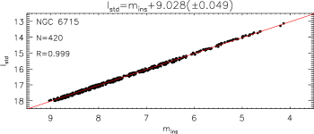
Figure 2: Standard I magnitude taken from the HST observations as a function of the instrumental $\mathrm{i}^{\prime}+\mathrm{z}^{\prime}$ magnitude. The red line is the fit that best matches the data and it is described by the equation in the title. The correlation coefficient is 0.999.

4 Variable star searches

Light curves for a total of 1405 stars were obtained with the DanDIA pipeline in the field covered by the reference image. To detect and extract the variable stars from all the non-variables, three automatic (or semi-automatic) techniques were employed. They are described in Sections 4.1, 4.2, and 4.3.

4.1 Root mean square

A diagram of root mean square (RMS) magnitude deviation against mean I magnitude (see top Fig. 3) was constructed for the cluster. In this diagram, we measure not only the photometric scatter for each star, but also the intrinsic variation of the variable stars over time, which gives them a higher RMS than the non-variables. The classification is indicated by the colour as detailed in Table 7. To select candidate variable stars, we fit a polynomial to the rms values as a function of magnitude and flag all stars with an rms greater than two times the model value.

4.2 $S_{B}$ statistic

A detailed discussion can be found about the benefits of using the $S_{B}$ statistic to detect variable stars (Figuera Jaimes et al., 2013) and RR Lyrae with Blazhko effect (Arellano Ferro et al., 2012). The $S_{B}$ statistic is defined as

$$S_{B}=\left(\frac{1}{NM}\right)\sum_{i=1}^{M}\left(\frac{r_{i,1}}{\sigma_{i,1}}+\frac{r_{i,2}}{\sigma_{i,2}}+...+\frac{r_{i,k_{i}}}{\sigma_{i,k_{i}}}\right)^{2},$$ (3)

where $N$ is the number of data points for a given light curve and $M$ is the number of groups formed of time-consecutive residuals of the same sign from a constant-brightness light curve model (e. g. mean or median). The residuals $r_{i,1}$ to $r_{i,k_{i}}$ correspond to the $i$th group of $k_{i}$ time-consecutive residuals of the same sign with corresponding uncertainties $\sigma_{i,1}$ to $\sigma_{i,k_{i}}$. The $S_{B}$ statistic is larger in value for light curves with long runs of consecutive data points above or below the mean, which is the case for variable stars with periods longer than the typical photometric cadence.

A plot of $S_{B}$ versus mean I magnitude is given for NGC 6715 (see bottom Fig. 3), variable stars are plotted in colour. To select candidate variable stars, the same technique employed in Section 4.1 was used, with the threshold also set at two times the model $S_{B}$ values.

4.3 Stacked difference image

Based on the results obtained using the DanDIA pipeline, a stacked difference image was built for NGC 6715 with the aim of detecting the difference fluxes that correspond to variable stars in the field of the reference image. The stacked image is the result of summing the absolute values of the difference images divided by the respective pixel uncertainty

$$S_{ij}=\sum_{k}\frac{|D_{kij}|}{\sigma_{kij}},$$ (4)

where $S_{ij}$ is the stacked image, $D_{kij}$ is the $k$th difference image, $\sigma_{kij}$ is the pixel uncertainty associated with each image $k$ and the indexes $i$ and $j$ correspond to pixel positions.

All of the variable star candidates obtained by using the RMS and $S_{B}$ diagrams explained in Sections 4.1 and 4.2 were inspected visually in the stacked image and by blinking the difference images to confirm or refute their variability.

5 Variable star classification

To define the type of variation in each of the variable stars found, several steps were done. First, we used their position in the colour-magnitude diagram (CMD; Fig. 4) as a reference for their evolutionary stage as most types of variable stars are placed in very well defined zones in the CMD. Second, we implemented a period search for each of the light curves by using the string method (Lafler & Kinman, 1965) and by minimising the $\chi^{2}$ in a Fourier analysis fit. Periods found and light curve shapes were also taken into account. Finally, to classify the variable stars, we used the conventions defined in the General Catalogue of Variable Stars (Samus et al., 2009).

In Table 7, the classification, corresponding symbols, and colours used in the plots throughout the paper are shown.

6 Colour magnitude diagram

As our sample has data available for only one filter, we decided to build the colour-magnitude diagram (CMD; see Fig. 4) by using the information available from the HST images at the ACS Globular Cluster Survey. The data used correspond to the V and I photometry obtained in Sirianni et al. (2005). The CMD was useful in classifying the variable stars, especially those with poorly defined light curves such as long period variables and semi-regular variables, as well as corroborating cluster membership.

7 NGC 6715 / C1851-305 / Messier 54

The details of all variable stars in our FoV that are discussed in this section are listed in Table 9, and all light curves are plotted in Figure 7.

Table 2: Convention used in the variable star classification of this work based on the definitions of the General Catalogue of Variable Stars (Samus et al., 2009).

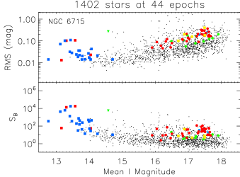
Figure 3: Root mean square (RMS) magnitude deviation (top) and $S_{B}$ statistic (bottom) versus the mean $I$ magnitude for the 1402 stars detected in the field of view of the reference image for NGC 6715. Coloured points follow the convention adopted in Table 7 to identify the types of variables found in the field of this globular cluster.

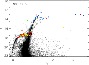
Figure 4: Colour magnitude diagram of the globular cluster NGC 6715 built with V and I magnitudes available in the ACS globular cluster survey extracted from HST images.

7.1 Known variables

This globular cluster has of the order of 200 known variable stars listed in the Catalogue of Variable Stars in Galactic Globular Clusters (CVSGGC; Clement et al., 2001). Most of them are of the RR Lyrae type but a few are long-period irregular, semi-regular, W Virginis, eclipsing binaries, and SX Phoenicis. To date four studies report variable star discoveries in this globular cluster: V1-V28 from Rosino (1952), V29-V82 from Rosino & Nobili (1958), V83-V117 from Layden & Sarajedini (2000), and V118-V211 from Sollima et al. (2010).

In the field of view covered by our reference image there are only five known variable stars (V112, V160, V173, V181, V192). All of them lie towards the edges of the image as can be seen in Figure 5. The star V112 was previously classified as long-period irregular. However, we were able to find a period of $\sim$ 100 days in the variability of this star and due to this we have reclassified it as a semi-regular variable. For V160, we were not able to produce a good phased light curve using the published period of 0.6194848 d. The discovery observations by Sollima et al. (2010) cover a time baseline of only 6 days. With our time baseline of more than two years, our derived periods are much more precise and the period found is in agreement with that found by the Optical Gravitational Lensing Experiment (OGLE, Udalski et al., 1992, see below). For V160, we list the OGLE period of 0.62813716 d in Table 9. For V173, we improved the period estimate over that from Sollima et al. (2010). For V181, we find a very different period with respect to the one estimated by Sollima et al. (2010). The new period of 0.877072 d makes this RR Lyrae the one with the longest period in the cluster. The phased light curve in Figure 7 is somewhat noisy because this variable is highly blended with a brighter star. The case of V192 is particularly interesting because the star was classified as RR1 with a period of 0.3986799 d. However, at the astrometric position reported for this star we found a RR Lyrae type RR0 with a period of 0.600373 d. This is also in agreement with the period and classification found by OGLE (see below) which we list in Table 9. Again, the phased light curve of this variable is noisy because of blending with a brighter star. It is clear then that the Sollima et al. (2010) periods and RR Lyrae classifications are not robust based on relatively few observations. We will discuss the consequences of this later on.

Recently, Montiel & Mighell (2010) announced 50 RR Lyrae candidates based on observations taken with the HST. However, the data obtained consist of 12 epochs covering only 8 hours, which made the study unsuitable for a period search and certainly some RR Lyrae stars will have been missed with such a short time baseline. No light curves were presented in their paper. Of these 50 candidate variable stars, 17 lie outside of our field of view (VC2, VC11-VC18, VC22, VC24, VC38, VC44, VC45, VC47-VC49). As pointed out in the Catalogue of Variable Stars in Galactic Globular Clusters (Clement et al., 2001), 11 of these candidates are previously known variables, thus VC2=V127, VC11=V162, VC12=V163, VC13=V95, VC14=V164, VC15=V142, VC17=V129, VC18=V179, VC44=V46, VC45=V148, and VC47=V76 (see also Appendix A). For 8 of their candidates in our field of view, we could not detect variations in our difference images at their coordinates (VC3, VC6, VC19, VC21, VC29, VC42, VC43, VC50), and we therefore cannot confirm their variability. We plot their positions in Figure 5 with a green square. Three of their candidates in our field of view, VC28, VC34 and VC46, are the known variables V181, V160 and V192, respectively. We confirm the variable nature of the remaining 22 candidates in our field of view, and we have assigned them “V” numbers as part of our study (see Section 7.2). Table 9 lists their VC identification in Column 2. We classify 18 of them as RR Lyrae stars, one as an eclipsing binary, and are unable to classify VC27, VC32, and VC33. We plot their positions in Figure 5 with a square symbol.

The study by McDonald et al. (2014) using the VISTA survey also covered the cluster and presents candidate variables based on typically $\sim$12-13 epochs spread over $\sim$100-200 days, which was insufficient to derive periods for many of them. Of the short period candidate variables listed in their Table 1, 18 are inside the field of view covered by our reference image. None of the bright long-period variables listed in their Table 2 and faint candidates listed in their Table 3 are inside the field covered in our study. Positions of these stars inside our field of view are plotted in Figure 5 with a red circle. It is worth noting that all of these candidates are located more toward the edges of the reference image. We detect variability in only two of the McDonald et al. (2014) candidates within our field of view (SPVSgr18550405-3028580 and SPVSgr18550386-3028593, which we assign V identifications as V229 and V263, respectively -see Section 7.2).

Similarly, the field of this cluster was also covered by OGLE, particularly with their OGLE-IV survey (Udalski et al., 2015). We found in this survey 15 of the variable stars studied in our work of which two are previously known variables (V160 and V192) and 13 are new discoveries by OGLE (we assigned the following V identifications: V227-V229, V233, V236, V237, V240, V244, V246, V250-V253). The OGLE light curves for these stars have typically $\sim$150 epochs covering a baseline of $\sim$2.5 years and OGLE derived precise periods for them. With our data we were also able to find the same periods and type of classification assigned by OGLE. The positions of these stars are plotted in Figure 5 with a blue colour. Again, it is worth noticing that all of these variables are located more toward the edges of the reference image. In the particular case of V229, V244, and V246, the pipeline was not able to detect these stars in the reference image but their variation is clear in the difference images. Their differential fluxes against phase are plotted in Figure 7. Finally, epochs, periods, mean magnitudes, amplitudes, and classifications for these three stars were taken from the OGLE database, although the number of data points listed in Table 9 correspond to our light curves.

In Appendix A (Table A), we provide the cross identifications for the previously known RR Lyrae stars in NGC 6715 between the CVSGGC (Clement et al., 2001), the variable star candidates from Montiel & Mighell (2010), and the OGLE RR Lyrae stars (Udalski et al., 2015).

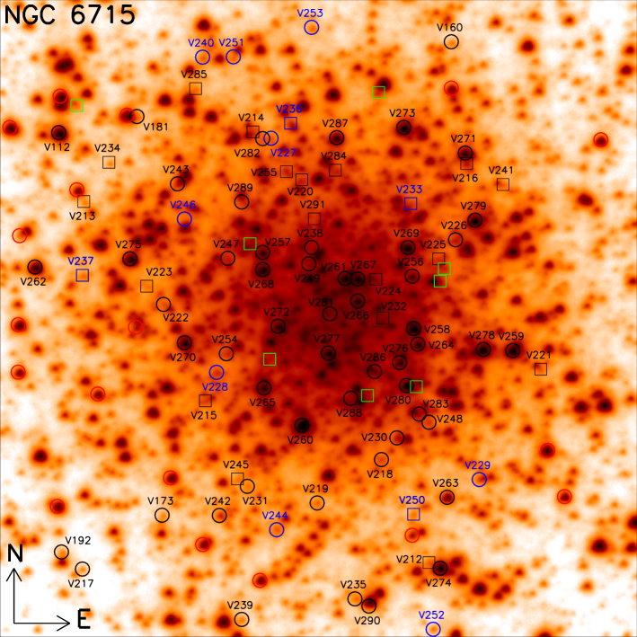
Figure 5: Finding chart for the globular cluster NGC 6715. The image used corresponds to the reference image constructed during the reduction. All known variables and new discoveries are labelled with their V numbers. Known variables, or new variables discovered in this work, are plotted with black symbols. Variables discovered by the OGLE survey are plotted with blue symbols. Those variables that were candidate variables from Montiel & Mighell (2010) are plotted using squares. Otherwise symbols are circles. Green squares and red circles, both without labels, are candidate variables from Montiel & Mighell (2010) and McDonald et al. (2014) respectively for which we do not detect variability in our survey. Image size is $\sim 40\times 40$arcsec².

7.2 New variables

After employing the methods described in Section 4, we were able to extract 67 new variable stars in the core of NGC 6715 of which 30 are RR Lyrae, 1 is a W Virginis star (CWA), 21 are long-period irregular, 3 are semi regular, 1 is an eclipsing binary, and 11 remain without classification.

7.2.1 RR Lyrae

V213-V226, V230-V232, V234-V235, V238-V239, V241-V243, V245, V247-V249, V254-V255: These 30 newly discovered variable stars are clear RR Lyrae variables. Their positions in the CMD, light curve shapes, periods, and amplitudes corroborate their variability type. We found that 17 are pulsating in the fundamental mode (RR0); 8 are pulsating in the first overtone (RR1); 1 is a double-mode pulsator (RR01) and 4 RR Lyrae remain with an uncetain subtype (3 RR0? and 1 RR1?). As shown in Table 9, their periods range from $\sim$0.28 d to $\sim$0.76 d with amplitudes between 0.06 and 1.69 mag.

The periodogram analysis for V221 showed two predominant frequencies typical of double mode RR Lyrae stars, one equivalent to the fundamental period $P_{0}=$ 0.459608 d and one equivalent to the first overtone period $P_{1}=$ 0.343828 d giving a period ratio $P_{1}/P_{0}=$ 0.748 which falls in the expected ratio range of $\sim 0.725$ to $\sim 0.748$ for this type of pulsating RR Lyrae stars (Netzel et al., 2015; Moskalik, 2013; Cox et al., 1983). Further data for a more detailed analysis of this star will be useful to corroborate its pulsational properties.

7.2.2 W Virginis

V256: Particularly interesting is the case of this star as its variation (and position in the CMD) do not follow the pattern found for the other variable stars studied and classified in this work. We found a very well phased light curve with a period of $\sim$14.771 d and an amplitude of 0.71 mag. This is the only bright variable star on the blue side of the colour-magnitude diagram far away from the red giant branch.

The properties found in the variation of this star and its position in the CMD match very well with the W Virginis type of variable star described in Samus et al. (2009), particularly with the subtype CWA which have periods longer than 8 days (see also Wallerstein, 2002). Although these types of stars have not been commonly found in globular clusters in contrast to RR Lyrae stars, they are not entirely uncommon. In the statistics of variable stars in Galactic globular clusters reported by Clement et al. (2001) it is possible to notice that 60 variable stars are Cepheids, which include Population II Cepheids, anomalous Cepheids, and RV Tauri stars. V256 is the first CWA star discovered in this cluster.

7.2.3 Long-period irregular

V260-V280: These 21 stars are located at the top of the red giant branch as shown with blue squares in Figure 4. Their amplitudes range from 0.05 to 0.46 mag. We found no clear periods for these stars. Due to this and also their position in the colour-magnitude diagram we classified them as long-period irregular. Light curves for all these variables are found in Figure 7.

7.2.4 Semi regular

V257-V259: Based on the position of these 3 stars in the colour-magnitude diagram (see Fig. 4), their periods, and the shape of their light curves, we have classified them as semi-regular. Light curves for these variables may be found in Figure 7. Their amplitudes range from $\sim$0.04 to $\sim$0.45 mag and their periods span between $\sim$20 and $\sim$150 d.

7.2.5 Eclipsing Binary

V212: The light curve variations for this star are very similar to those presented in eclipsing binary systems. We found that the amplitude of the deeper eclipse is of the order of $\sim$0.8 mag and the amplitude of the secondary eclipse is $\sim$0.5 mag. The phased light curve shown in Figure 7 represented a period of $P=$ 0.202144 d.

7.2.6 Other variable stars

V281-V285: These 5 stars are clear variable stars. They show clear variability by blinking the difference images. They have amplitudes between 0.45 and 0.94 mag. Several attempts to determine periods for these stars were done without success. Due to this their light curves in Figure 7 are plotted against HJD. We note that the variable source V281 is ony $\sim$0.24 arcsec from the photometric centre of the cluster as measured by Goldsbury et al. (2010).

V286: Towards the beginning of the 2013 data, we found that the flux of this star was increasing to a maximum at $\sim$2456464.9081 d of about $\sim$39400 ADU/s on the flux scale of the reference image, corresponding to a peak magnitude of $\sim$15.04 mag. After that, its flux strongly decreased during the rest of the observational campaign. During 2014 and 2015, we found that the object seems to be at baseline and it is not detected in the original images.

The centre of NGC 6715 is $\sim$4.45 arcseconds from this source. Also, at a distance of 3.73 arcseconds, there is a X-ray source studied by Wrobel et al. (2011) using data from Chandra and Hubble Space Telescope. Given the relatively small astrometric uncertainties in these positions, V286 is not associated with either. The nature and classification of this variable will need further studies, and it will remain without classification in this work.

V287-V291: These 5 stars were not detected by the pipeline in the reference image. Unfortunately, there are no light curves available in the OGLE database for these stars, but their variations are clear in the difference images. In Figure 7 their differential fluxes against HJD are plotted. As we were not able to produce phased light curves for them, they will remain without classification until future studies are done.

8 Oosterhoff dichotomy

In this work we discovered 30 new RR Lyrae, and OGLE also discovered 17 more (of which 13 are inside our FoV). After removing the stars without a secure classification, there are 33 new RR0 and 9 new RR1 stars, which represent a significant increment in the known RR Lyrae population. The vast majority of these new RR Lyrae stars are cluster members since we have studied the core of NGC 6715. Hence it is pertinent to recalculate the mean periods and number ratios of the RR Lyrae stars to see if it modifies the current conclusions about the Oosterhoff type of NGC 6715.

However, we note that NGC 6715 lies projected against the Sagittarius Dwarf Spheroidal galaxy and behind the Galactic bulge. Therefore, the sample of RR Lyrae stars in the field of the cluster is a mixture of cluster members, Bulge stars, and Sgr dSph stars. Towards the centre of NGC 6715, the cluster member RR Lyraes dominate, but limiting our sample to the cluster core also reduces the number of RR Lyraes that can be used to calculate the mean periods and number ratios. Hence, in Figure 6, we have plotted the total number of RR Lyrae stars, the mean period of the RR0 stars, the mean period of the RR1 stars, and the number ratio of the RR1 to all RR Lyrae stars (nRR1/(nRR0 + nRR1)), all as a function of distance from the cluster centre (RA(J2000) = 18:55:03.33; Dec(J2000)=$-$30:28:47.5; Goldsbury et al., 2010). To convert angles on the sky into distances in parsecs we used the distance from the Sun to NGC 6715 of 26500 pc (Harris, 1996, 2010 version). The inner and outer red vertical lines are the tidal radii estimated by McLaughlin & van der Marel (2005) based on King (1966) and Wilson (1975) models, respectively. The horizontal black lines correspond to the OoI (solid) and OoII (dashed) types given by Smith (1995) in his Table 3.2. We only used RR Lyrae stars with certain classifications (i.e. published phased light curves with reliable period estimates).

Figure 6 clearly shows that within the range of the two estimates of the tidal radii, where the RR Lyrae stars from the cluster still dominate, the values of $<P_{\mathrm{RR0}}>$, $<P_{\mathrm{RR1}}>$ and nRR1/(nRR0 + nRR1) are intermediate between those expected for OoI and OoII clusters. We obtain $<P_{\mathrm{RR0}}>$=0.613529 d, $<P_{\mathrm{RR1}}>$=0.334107 d, and nRR1/(nRR0 + nRR1)= 0.24050633 when calculated for the 79 RR Lyraes within the outer estimate of the tidal radius (i.e. 380 pc). The contaminating RR Lyrae populations have ($<P_{\mathrm{RR0}}>$, $<P_{\mathrm{RR1}}>$)=(0.556 d, 0.310 d) and ($<P_{\mathrm{RR0}}>$,$<P_{\mathrm{RR1}}>$)=(0.574 d, 0.322 d) for the Bulge and Sgr dSph, respectively (Soszyński et al., 2011; Cseresnjes, 2001), placing them in the OoI region in the $<P_{\mathrm{RR0}}>$-metallicity diagram of Catelan (2009). This explains why the values of $<P_{\mathrm{RR0}}>$ and nRR1/(nRR0 + nRR1) tend towards the OoI values beyond the outer estimate of the tidal radius. The value of $<P_{\mathrm{RR1}}>$ is hardly influenced though because there are only 6 RR1 stars beyond the outer estimate of the tidal radius. Hence the new RR Lyrae discoveries in this paper have served to confirm that NGC 6715 is of intermediate Oosterhoff type.

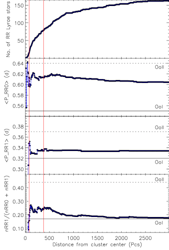
Figure 6: The number of RR Lyraes, mean periods, and number ratios as a function of the distance from the cluster centre. The red lines correspond to the tidal radii calculated by McLaughlin & van der Marel (2005).

9 Conclusions

The globular cluster NGC 6715 turns out to be a very interesting stellar system, for which images with the highest angular resolution have ever been obtained so far with ground-based telescopes. The use of the EMCCD and shift-and-add technique was demonstrated to be an excellent procedure to minimise the effect of the atmospheric turbulence which is one of the main constraints when doing ground-based observations. Thanks to this and the use of difference image analysis it was possible to obtain high-precision time series photometry in the core of this cluster down to $I\sim$18.3 mag.

A total of 1405 stars in the field covered by the reference image were statistically studied for variable star detection. We presented light curves for 17 previously known variables that were found toward the edges of the reference image (16 RR Lyrae and 1 SR). We also discovered 67 new variable stars, which consist of 30 RR Lyrae, 21 long-period irregular, 3 semi-regular, 1 W Virginis, 1 eclipsing binary, and 11 unclassified stars. We estimated periods and ephemerides for all variable stars in the field of our reference image. Our new RR Lyrae star discoveries help confirm that NGC 6715 is of intermediate Oosterhoff type. Finally, our photometric measurements for all variable stars studied in this work are available in electronic form through the Strasbourg Astronomical Data Centre.

Table 3: Ephemerides and main characteristics of the variable stars in the field of globular cluster NGC 6715. Column 1 is the id assigned to the variable star, Column 2 is a previously known id assigned to the stars (5 digit numbers correspond to OGLE identifications of the form OGLE-BLG-RRLYR-NNNNN), Columns 3 and 4 correspond to the right ascension and declination (J2000), Column 5 is the epoch used, Column 6 is the period measured in this work unless the variable is an OGLE star in which case we use their period, Column 7 is median magnitude, Column 8 is the peak-to-peak amplitude in the light curve, Column 9 is the number of epochs and Column 10 is the classification of the variable. The numbers in parentheses indicate the uncertainty on the last decimal place of the period.

^aEpochs, periods, mean magnitudes, amplitudes, and classifications taken from OGLE database       ^b=SPVSgr18550405-3028580; ^c=SPVSgr18550386-3028593; ^d=Peak magnitude       Concluded

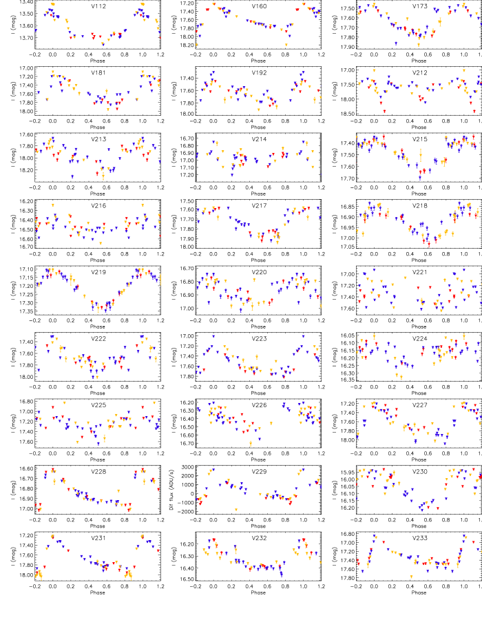
(a)

Figure 7: Light curves of the known and new variables discovered in globular cluster NGC 6715. Red, blue, and yellow triangles correspond to the data obtained during the years 2013, 2014, and 2015, respectively. For V229, V244, V246, V286-V291, we plot the quantity $f_{\mathrm{diff}}(t)/p(t)$ since a reference flux is not available.

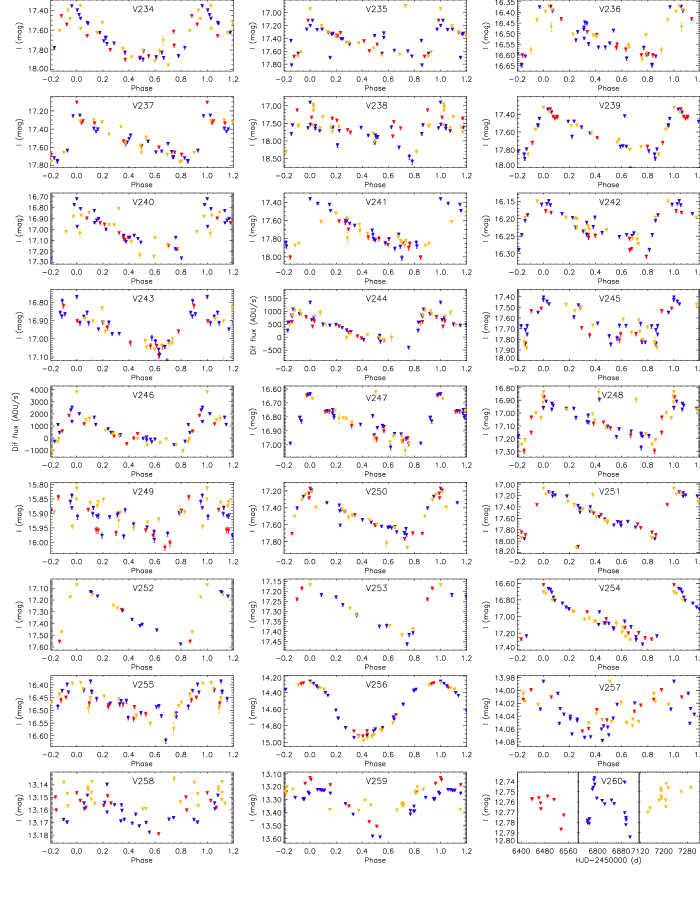
(b)

Figure 7: Light curves of the known and new variables discovered in globular cluster NGC 6715. Red, blue, and yellow triangles correspond to the data obtained during the years 2013, 2014, and 2015, respectively. For V229, V244, V246, V286-V291, we plot the quantity $f_{\mathrm{diff}}(t)/p(t)$ since a reference flux is not available (cont.).

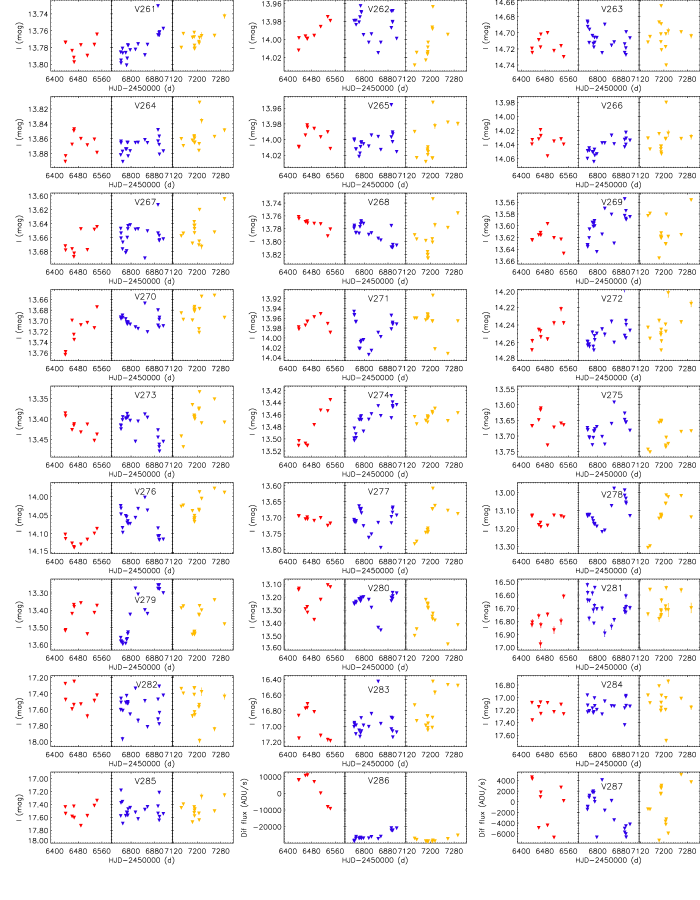
(c)

Figure 7: Light curves of the known and new variables discovered in globular cluster NGC 6715. Red, blue, and yellow triangles correspond to the data obtained during the years 2013, 2014, and 2015, respectively. For V229, V244, V246, V286-V291, we plot the quantity $f_{\mathrm{diff}}(t)/p(t)$ since a reference flux is not available (cont.).

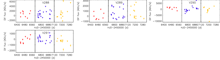
(d)

Figure 7: Light curves of the known and new variables discovered in globular cluster NGC 6715. Red, blue, and yellow triangles correspond to the data obtained during the years 2013, 2014, and 2015, respectively. For V229, V244, V246, V286-V291, we plot the quantity $f_{\mathrm{diff}}(t)/p(t)$ since a reference flux is not available (cont.).

Appendix A Cross identification between variables

Table 4: Cross identification between the RR Lyrae variables listed by the CVSGGC (Clement et al., 2001), the variable star candidates from Montiel & Mighell (2010), and the OGLE RR Lyrae stars (Udalski et al., 2015)