The JCMT Gould Belt Survey: Evidence for Dust Grain Evolution in Perseus Star-forming Clumps

Abstract

The dust emissivity spectral index, , is a critical parameter for deriving the mass and temperature of star-forming structures, and consequently their gravitational stability. The  value is dependent on various dust grain properties, such as size, porosity, and surface composition, and is expected to vary as dust grains evolve. Here we present , dust temperature, and optical depth maps of the star-forming clumps in the Perseus Molecular Cloud determined from fitting SEDs to combined Herschel and JCMT observations in the 160 µm, 250 µm, 350 µm, 500 µm, and 850 µm bands. Most of the derived , and dust temperature values fall within the ranges of 1.0 - 2.7 and 8 - 20 K, respectively. In Perseus, we find the  distribution differs significantly from clump to clump, indicative of grain growth. Furthermore, we also see significant, localized  variations within individual clumps and find low  regions correlate with local temperature peaks, hinting at the possible origins of low  grains. Throughout Perseus, we also see indications of heating from B stars and embedded protostars, as well evidence of outflows shaping the local landscape.

1 Introduction

Thermal dust emission is an excellent tracer of cold, star-forming structures. When observed in wide bands, the spectral energy distributions (SEDs) of these structures are dominated by optically thin, thermal dust emission at far-infrared and sub-millimeter wavelengths. The column densities, and consequently the masses, of star-forming structures can thus be estimated from their dust emission by assuming a dust opacity, $\kappa_{\nu}$, and a dust temperature, $T_{d}$. The dust opacity at frequencies $\nu\lesssim 6$ THz, however, has a frequency dependency typically modelled as a power law, characterized by the emissivity spectral index,  (e.g., Hildebrand 1983). Depending on the dust model, $\kappa_{\nu}$ can be uncertain by up to a factor of 3 - 7 at a given frequency between 0.3 - 3 THz (see Figure 5 in Ossenkopf & Henning 1994). The ability to determine mass precisely, therefore, depends heavily on how well  and the normalization reference opacity, $\kappa_{\nu_{0}}$, can be constrained.

Measuring  is difficult because it requires the SED shape of the dust emission to be well determined, especially when $T_{d}$ is not already known from independent measurements. The ability to determine the true SED shape can be particularly susceptible to noise in the data and temperature variations along the line of sight, resulting in erroneous measurements of  and $T_{d}$ (e.g., Shetty et al. 2009a; Shetty et al. 2009b; Kelly et al. 2012). For this reason, a fixed  value of $\sim 2$ has commonly been adopted in the literature, motivated by both observations of diffuse interstellar medium (ISM; e.g., Hildebrand 1983) and grain emissivity models (e.g., Draine & Lee 1984).

Given that  is an optical property of dust grains and can depend on various grain properties such as porosity, morphology, and surface composition, the  value of a dust population may be expected to change as the population evolves. Indeed, observations have shown that dust within protostellar disks have  $\simeq 1$ (e.g., Beckwith & Sargent 1991), which is substantially lower than the diffuse ISM value ($\sim 2$). Furthermore, a wide range of  values ($1\lesssim$ $\lesssim 3$) has been reported in many observations of star-forming regions on smaller scales ($\lesssim 2^{\prime}$; e.g., Shirley et al. 2005, 2011; Friesen et al. 2005; Kwon et al. 2009; Schnee et al. 2010; Arab et al. 2012; Chiang et al. 2012), as well as a few lower resolution observations on larger scales of a cloud (e.g., Dupac et al. 2003; Planck Collaboration et al. 2011). These results suggest that dust grains in star-forming regions can evolve significantly away from its state in the diffuse ISM, prior to being accreted onto protostellar disks.

Recent large far-infrared/sub-millimeter surveys of nearby star-forming clouds such as the Herschel Gould Belt Survey (GBS; André et al. 2010) and the James Clerk Maxwell Telescope (JCMT) GBS (Ward-Thompson et al. 2007) have provided unprecedented views of star-forming regions at resolutions where dense cores and filaments are resolved ($\lesssim 0.5^{\prime}$). Despite this advancement, only a few studies (e.g., Sadavoy et al. 2013; Schnee et al. 2014; Sadavoy et al. 2016) have attempted to map out  at resolutions similar to these surveys over large areas. Such  measurements can be very valuable in providing more accurate mass and temperature estimates, and consequently gravitational stability estimates, of the structures revealed in these surveys. While the Herschel GBS multi-band data may seem ideal for making  measurements in cold star-forming regions at first, Sadavoy et al. (2013) demonstrated that Herschel data alone are insufficient and longer wavelength data (e.g., JCMT 850 µm observations) are needed to provide sufficient constraints on .

Here we present the first results of the JCMT GBS 850 µm observation with the Sub-millimetre Common User Bolometer Array 2 (SCUBA-2) towards the Perseus Molecular Cloud as a whole. Employing the technique developed by Sadavoy et al. (2013) for combining the Herschel and JCMT GBS data, we simultaneously derive maps of $T_{d}$, , and optical depth at 300 µm, $\tau_{300}$, in the Perseus star-forming clumps by fitting modified blackbody SEDs to the combined data. We investigate the robustness and the uncertainties of our SED fits, and perform a detailed analysis of the derived parameter maps in an attempt to understand the local environment. In particular, we characterize the observed variation in  and discuss the potential physical driver behind such evolution.

In this paper, we describe the details of our observation and data reduction in Section 2, and our SED-fitting method in Section 3. The results, including the parameter maps drawn from SED fits, are presented in Section 4. We discuss the implication of our results in Section 5, with regards to radiative heating (Section 5.1), outflow feedback (Section 5.2), and dust grain evolution (Section 5.3). We summarize our conclusions in Section 6.

2 Observations

2.1 JCMT: SCUBA-2 Data

Table 1: Details of the observed PONG regions

Scan Name	RA	DEC	Clump	Weather Grade	Number of Scans
B5	03:47:36.92	+32:52:16.5	B5	2	6
IC348-E	03:44:23.05	+32:01:56.1	IC 348	1	4
IC348-C	03:42:09.99	+31:51:32.5	IC 348	2	6
B1	03:33:10.75	+31:06:37.0	B1	1	4
NGC1333-N	03:29:06.47	+31:22:27.7	NGC 1333	1	4
NGC1333	03:28:59.18	+31:17:22.0	NGC 1333	2	1
NGC1333-S	03:28:39.67	+30:53:32.6	NGC 1333	2	6
L1455-S	03:27:59.43	+30:09:02.1	L1455	1	4
L1448-N	03:25:24.56	+30:41:41.5	L1448	1	4
L1448-S	03:25:21.48	+30:15:22.9	L1451	2	6

Note. — The names, center coordinates, targeted clump names, and the weather grades of the individual observations made with the PONG1800 scan pattern. Clumps in the Table are ordered from east to west.

Wide-band 850 µm observations of Perseus were taken with the SCUBA-2 instrument (Holland et al. 2013) on the JCMT as part of the JCMT GBS program (Ward-Thompson et al. 2007). We included observations that were taken in the SCUBA-2 science verification (S2SV) and the main SCUBA-2 campaign of the GBS program, i.e., in October 2011, and between July 2012 and February 2014, respectively. As with the rest of the survey, Perseus regions were individually mapped using a standard PONG1800 pattern (Kackley et al. 2010, Holland et al. 2013, Bintley et al. 2014) that covers a circular region $\sim 30^{\prime}$ in diameter.

Our observations covered the brightest star-forming clumps found in Perseus, namely B5, IC 348, B1, NGC 1333, L1455, L1448, and L1451, listed here in order of east to west. Table 1 shows the names and center coordinates of the observed PONG1800 maps, along with the weather grades in which they were observed. Based on priority, each planned PONG target was observed either four times under very dry conditions (Grade 1; $\tau_{225}<0.05$) or six times under slightly less dry conditions (Grade 2; $\tau_{225}=0.05-0.07$) to reach the targeted survey depth of 5.4 mJy beam^-1 for 850 µm. The ‘northern’ PONG region of NGC 1333 is the only exception, containing one extra S2SV PONG900 map observed under Grade 2 weather. As with Sadavoy et al. (2013), we adopted $14.2^{\prime\prime}$ as our effective Gaussian FWHM beamwidth for the 850 µm data based on the two components of the SCUBA-2 beam obtained from measurements.

All SCUBA-2 data observed for the JCMT GBS program were reduced with the makemap task from the Starlink SMURF package (Version 1.5.0; Jenness et al. 2011; Chapin et al. 2013) following the JCMT GBS Internal Release 1 (IR1) recipe, consistent with other JCMT GBS first-look papers (e.g., Salji et al. 2015). The ¹²CO $J=3-2$ line contribution to the 850 µm data is further removed with the JCMT Heterodyne Array Receiver Program (HARP) observations (see Buckle et al. 2009) as part of the IR1 reduction. Weather-dependent conversion factors calculated by Drabek et al. (2012) were applied to the HARP data prior to the CO subtraction. For more details on the IR1 reduction and CO subtraction, see Sadavoy et al. (2013) and Salji et al. (2015).

2.2 Herschel: PACS and SPIRE Data

The Perseus region was observed with the PACS (Photodetector Array Camera and Spectrometer; Poglitsch et al. 2010) instrument and the SPIRE instrument (Spectral and Photometric Imaging Receiver; Griffin et al. 2010; Swinyard et al. 2010) as part of the Herschel GBS program (André & Saraceno 2005; André et al. 2010; Sadavoy et al. 2012, 2014), simultaneously covering the 70 µm, 160 µm, 250 µm, 350 µm, and 500 µm wavelengths using the fast ($60^{\prime\prime}/$s) parallel observing mode. The observation of the western and the eastern portions of Perseus took place in February 2010 and February 2011, respectively, covering a total area of $\sim 10$ deg². We reduced our data with Version 10.0 of the Herschel Interactive Processing Environment (HIPE; Ott 2010) using modified scripts written by M. Sauvage (PACS) and P. Panuzzo (SPIRE) and PACS Calibration Set v56 and the SPIRE Calibration Tree 10.1. Version 20 of the Scanamorphos routine (Roussel 2013) was used in addition to produce the final PACS maps. The final Herschel maps have resolutions of $8.4^{\prime\prime}$, $13.5^{\prime\prime}$, $18.2^{\prime\prime}$, $24.9^{\prime\prime}$, and $36.3^{\prime\prime}$ in order of shortest to longest wavelength. For more details on the Herschel observations of Perseus, see Pezzuto et al. (2012), Sadavoy (2013), and Pezzuto et al. (2016, in prep.).

The SCUBA-2 data are spatially filtered to remove slow, time-varying noise common to all bolometers, such as atmospheric emission to which ground-based sub-millimeter observations are susceptible. For effective combinations, we filtered the Herschel data using the SCUBA-2 map-maker makemap (Jenness et al. 2011; Chapin et al. 2013) following the method described by Sadavoy et al. (2013) to match the spatial sensitivity of the Herschel data to that of the SCUBA-2 observations. Given that any zero-point flux offsets in the Herschel data are removed by the spatial filtering along with other large-scale emission, no offset correction was applied to our Herschel data. Further details on the parameters used for filtering the Herschel data are described in Chen (2015)

3 SED-fitting

We modelled our dust spectral energy distributions as a modified blackbody function in the optically thin regime in the form of

$$I_{\nu}=\tau_{\nu_{0}}\left(\nu/\nu_{0}\right)^{\beta}B_{\nu}(T_{d})$$ (1)

where $\tau_{\nu_{0}}$ is the optical depth at frequency $\nu_{0}$, $\beta$ is the dust emissivity power law index, and $B_{\nu}(T_{d})$ is the blackbody function at the dust temperature $T_{d}$. By adopting a dust opacity value, $\kappa_{\nu_{0}}$, one can further derive the gas column densities as the following using the $\tau_{\nu_{0}}$ values:

$$N(H_{2})=\frac{\tau_{\nu 0}}{\mu m_{H_{2}}\kappa_{\nu 0}}$$ (2)

where $\mu$ is the mean molecular weight of the observed gas and $m_{H_{2}}$ is the mass of a molecular hydrogen in grams. For this study, we adopted a reference frequency $\nu_{0}=1$ THz (300 µm), $\mu=2.8$, and $\kappa_{\nu_{0}}=0.1$ cm² g^-1, consistent with assumptions made by the Herschel GBS papers (e.g., André et al. 2010).

We convolved the CO-removed SCUBA-2 850 µm data and the spatially-filtered Herschel data with Gaussian kernels to a common resolution of $36.3^{\prime\prime}$ to match that of the 500 µm Herschel map, the lowest resolution of our data. We re-aligned and re-gridded the convolved maps to the original 500 µm Herschel map, which has $14^{\prime\prime}\times 14^{\prime\prime}$ pixels. The 70 µm data were excluded from our SED fitting because that emission may trace a population of very small dust grains that are not in thermal equilibrium with the dust traced by the longer wavelength emission (Martin et al. 2012).

Following Sadavoy et al. (2013), we applied color correction factors of 1.01, 1.02, 1.01, and 1.03 to the 160 µm, 250 µm, 350 µm, and 500 µm Herschel data, respectively, to account for the spectral variation within each band. The correction factors are taken from the averaged values calculated from SED models with specific $T_{d}$ and  values (i.e., 10 K $\leq T_{d}\leq 25$ K and $1.5\leq$ $\leq 2.5$). The color calibration uncertainties associated with these color correction factors are 0.05, 0.008, 0.01, and 0.02 times that of the color corrected values, respectively.

For each pixel of the map with signal-to-noise ratios (SNRs) $\geq 10$ in all five bands, we fitted a modified blackbody function (Equation 1) to get best estimates of , $T_{d}$, and $\tau_{\nu_{0}}$. We employed the minimization of $\chi^{2}$ method using the optimize.curve_fit routine from the Python SciPy software package, which uses the Levenberg-Marquardt algorithm for minimization. The flux uncertainties were calculated as the quadrature sum of the color calibration uncertainties and the map sensitivities (see Table 2), and were adopted as standard errors for the $\chi^{2}$ calculation. For each clump, we adopted the 1-$\sigma$ rms noise measured from a relatively smooth, emission-free region within the convolved, filtered maps as the map sensitivity.

In addition to color calibration uncertainties and map noise, we followed Könyves et al. (2015) in adopting 20% as the absolute flux calibration uncertainties for the PACS 160 µm band and 10 % for the SPIRE bands. We also followed Sadavoy et al. (2013) in adopting 10% as the absolute flux calibration uncertainty in the SCUBA-2 850 µm band. We note that 10% is a conservative estimate of the absolute flux calibration uncertainties for extended sources and the calibration accuracy of point sources are much higher ($<7\%$ for PACS bands, Balog et al. 2014; $\sim 5\%$ for SPIRE bands, Bendo et al. 2013; $<8\%$ for SCUBA-2 850 µm band).

The flux calibration uncertainties are assumed to be correlated between the bands within an instrument, and we employed a simple Monte Carlo method to determine the most probable fit given the assumed calibration uncertainties based on a thousand instances. The resulting probability distribution for a given pixel was collapsed onto the $T_{d}$ and  axes separately and fitted with a Gaussian distribution to determine the associated 1-$\sigma$ uncertainties of the derived $T_{d}$ and . Due to the asymmetric distribution of the derived $\tau_{300}$, we used the best fit $\tau_{300}$ from another SED fit with $T_{d}$ and  fixed at their mean best-fit values from their respective Gaussian fits. We derived the uncertainty in $\tau_{300}$ from the covariance of this final fit. For more details on the SED fitting and how the flux calibration uncertainties are handled, see Sadavoy et al. 2013 and Chen 2015.

The  and $T_{d}$ derived using the minimization of $\chi^{2}$ method can produce artificial anti-correlations due to the shape of the assumed SED becoming degenerate in the presence of moderate noise (Shetty et al. 2009b; 2009a) and flux calibration uncertainties. Detailed analysis of these correlated uncertainties are presented in Appendix A. To ensure the robustness of our results, we rejected pixels with  uncertainties $>30\%$, where the fits to the SED are often poor and the  and $T_{d}$ uncertainties occupy a distinct part of the parameter space relative to the main population. We also removed isolated regions that contained less than 4 pixels and where Gaussian fits to the derived  and $T_{d}$ distributions from the Monte Carlo simulation were poor.

Table 2: Noise levels in the Perseus data

Band	160 µm	250 µm	350 µm	500 µm	850 µm
B5	60	50	30	20	20
IC 348	150	110	50	20	40
B1	80	90	60	30	30
NGC 1333	50	60	30	20	30
L1455	60	70	50	20	30
L1448	60	50	30	20	30
L1451	60	50	30	20	30

Note. — The approximate 1-$\sigma$ rms noise levels (mJy beam^-1) of the convolved, spatially filtered maps at the resolution of $36.3^{\prime\prime}$ for different Perseus clumps. The rms noise values were measured in a relatively smooth, emission-free region of the filtered clump maps.

4 Results

4.1 Reduced Data

We present the reduced SCUBA-2 850 µm maps of the B5, IC 348, B1, NGC 1333, L1455, L1448, and L1451 clumps in Figure 1. For a comparison, we also present the reduced, unfiltered SPIRE 250 µm map in Figure 2, cropped to match the same regions shown in Figure 1. For the complete set of reduced, unfiltered PACS and SPIRE maps of Perseus, see Pezzuto et al. (2016, in prep.).

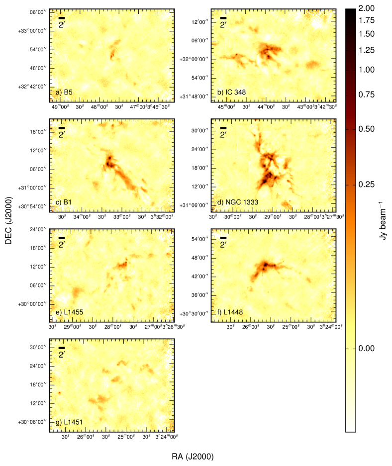
Figure 1: SCUBA-2 850 µm maps of the seven Perseus clumps, ordered from east to west and cropped to focus on the brightest regions. The flux are shown on a log scale from -0.03 Jy beam^-1 to 2.0 Jy beam^-1.

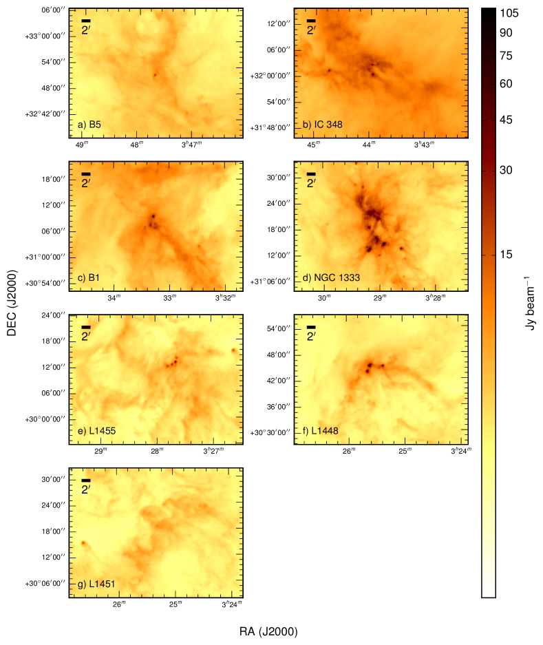
Figure 2: Unfiltered SPIRE 250 µm maps over the same regions shown in Figure 1. The flux are shown on a log scale from 0.05 Jy beam^-1 to 110 Jy beam^-1.

4.2 Derived Dust Temperatures

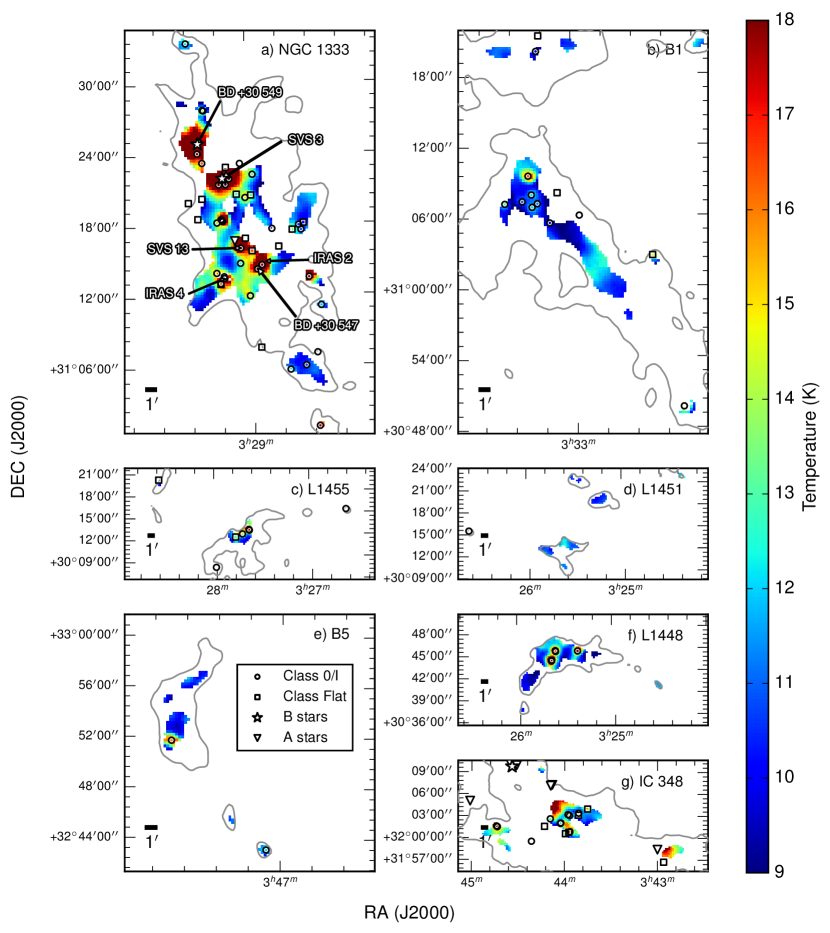
Figure 3: Derived dust temperature maps of the seven Perseus clumps, with the colors scaled linearly from 9 K to 18 K. B and A stars in the region are denoted with star and triangle symbols, respectively. The Class 0/I and Flat YSOs identified in Dunham et al.’s Gould Belt catalogue (2015) are denoted by circles and squares, respectively. Contours of the unfiltered Herschel 500 µm emission at 1.5 Jy beam^-1 are overlaid on the maps in grey.

Figure 3 shows the $T_{d}$ maps for all seven Perseus clumps overlaid with positions of embedded young stellar objects (YSOs), B stars, and A stars. The YSOs shown here are Class 0/I (circles) and Flat (squares) protostars identified from the Spitzer Gould Belt catalogue of mid-infrared point sources (Dunham et al. 2015). The B and A stars identified in various catalogs (referenced in the SIMBAD database, Wenger et al. 2000) are labelled with star and triangle symbols, respectively. Contours of the unfiltered Herschel 500 µm emission at 1.5 Jy beam^-1 are overlaid on the maps in grey. As demonstrated in Appendix A, the uncertainty in the $T_{d}$ measurement due to flux calibration uncertainties is dependent on $T_{d}$. The typical uncertainties at $T_{d}$ values of $<12$ K, 12 - 15 K, 15 - 20 K, and 20 - 30 K are 0.9 K, 1.5 K, 2.5 K, and 5.0 K respectively. The derived $T_{d}$ values at $T_{d}>30$ K are poorly constrained and typically have uncertainties of $\gtrsim 10$ K. Our derived $T_{d}$ values are systematically lower than those obtained from unfiltered Herschel data due to the preferential removal of the warm, diffuse dust emission by the spatial filtering. See Chen (2015) for further details on the bias introduced by the spatial filtering.

The $T_{d}$ structures seen in Figure 3 often appear as circular, localized peaks overlaid on relatively cold backgrounds ($\sim 10-11$ K). Nearly all localized $T_{d}$ peaks are coincident with at least an embedded YSO or a B star along their respective lines of sight, indicating that these objects are likely the source of local heating. The few $T_{d}$ peaks that do not contain an embedded YSO, B star, or A star are all located in IC 348 and partially on the map edges. These $T_{d}$ peaks may be the result of local heating by sources outside of the map such as the nearby A star shown in Figure 3 or the nearby star cluster.

The region just southeast of IRAS 2 in NGC 1333 also appears relatively warm ($\sim 14-15$ K) with no clear source of localized heating. While the star BD +30 547 (a.k.a., ASR 130, SSV 19) adjacent to IRAS 2B has often been classified as a foreground late type star (e.g., G2 IV, Cernis 1990), Aspin (2003) suggested that it may be a late-B V star with a cool faint companion, making BD +30 547 a potential source of heating in this region.

Interestingly, not all embedded YSOs are coincident with localized temperature peaks. This result is in agreement with that found by Hatchell et al. (2013) in NGC 1333. Out of the 61 embedded YSOs located within the temperature maps of Perseus clumps, only seven are not coincident with local temperature peaks. Some of these YSOs may be too faint, embedded, or young to have warmed their surrounding dust significantly. Alternatively, they could be more-evolved, less-embedded YSOs misidentified as Class 0/I or Class Flat objects, potentially due to line-of-sight confusion.

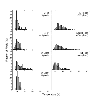
Figure 4: Histograms of derived $T_{d}$ values in the seven Perseus clumps. All the pixels within a clump are shown in light grey while the pixels within a $72.6^{\prime\prime}$ diameter (i.e., two Herschel 500 µm beam widths) centered on a Class 0/I and Flat YSOs are shown in dark grey.

Figure 4 shows histograms of derived dust temperatures, $T_{d}$, in each of the Perseus clumps. The light and dark grey histograms represent all the pixels within a clump and the pixels found within a $72.6^{\prime\prime}$ diameter (i.e., two Herschel 500 µm beam widths) area centered on a Class 0/I and Flat YSOs, respectively. Globally, the $T_{d}$ distributions of Perseus clumps all share two characteristic features: a primary low $T_{d}$ peak and a high $T_{d}$ tail. L1451 is the only clump without a high $T_{d}$ tail. All clumps have their primary $T_{d}$ peaks located at $\sim 10.5$ K, with the exception of IC 348 which has a temperature peak at $\sim 11.5$ K. The former is consistent with the typical $T_{d}$ seen in NGC 1333 (Hatchell et al. 2013), the kinetic temperatures observed towards dense cores in Perseus with ammonia lines (Rosolowsky et al. 2008; Schnee et al. 2009), and the isothermal $T_{d}$ of prestellar cores in other clouds (Evans et al. 2001).

As shown in Figure 4, nearly all the pixels found in the high $T_{d}$ tails of the overall distribution (light grey) of B5, B1, L1455, and L1448 are located within a $72.6^{\prime\prime}$ diameter area centered on an embedded YSO (dark grey), indicating that these YSOs are indeed the main source of heating in these clumps. While protostellar heating also appears to be significant in IC 348 and NGC 1333, as seen in the $T_{d}$ maps (Figure 3), only slightly less than half of the high $T_{d}$ pixels in these two clumps are found near embedded YSOs. The remainder of the pixels in the high $T_{d}$ tails of the distributions are likely from dust externally heated by B stars and nearby star clusters instead. No embedded YSO is found near pixels in L1451 where the SEDs were fitted. This lack of local heating sources likely explains why L1451 does not have a high $T_{d}$ tail.

Looking from another prespective, nearly all the pixels surrounding embedded YSOs (dark grey) in B5, L1455, and L1448 are found in the high $T_{d}$ tail of the overall distribution (light grey). This situation, however, is not seen in IC 348, B1, and NGC 1333, where a large fraction of the pixels near the embedded YSOs are found below $\sim 13$ K, near the 10.5 K $T_{d}$ peak. These low $T_{d}$ pixels are associated with the embedded YSOs not found towards the locally heated regions, or in some cases (e.g., B1) towards localized $T_{d}$ peaks that appear relatively cool.

Our derived $T_{d}$ values do not consistently drop off near map edges. This result indicates that our $T_{d}$ derivation is less susceptible to the edge effects caused by the large-scale filtering seen in the $T_{d}$ map of NGC 1333 derived by Hatchell et al. (2013) using the 450 µm and 850 µm data from the early SCUBA-2 shared risk observations. The north-western edge of our NGC 1333 map was the only exception, where the edge of the fitted map lies near the edge of the external mask used for the data reduction and spatial filtering. Nevertheless, the regions in Perseus where SEDs were fit are typically located well within the adopted external masks and are therefore unlikely to have experienced such a problem. We improved $T_{d}$ derivations in NGC 1333 with respect to Hatchell et al.’s analysis by using four additional bands from Herschel and allowing  to vary. Furthermore, the JCMT GBS data used here were taken with longer integration time with the full SCUBA-2 array instead of just one sub-array and had less spatial filtering. At $T_{d}\sim 10$ K, Hatchell et al.’s $T_{d}$ uncertainties due to flux calibration alone is $\sim 1.2$ K, whereas our typical uncertainty is $\sim 0.9$ K.

The appearance of our derived $T_{d}$ map of B1 is morphologically consistent with that derived by Sadavoy et al. (2013) using the same observations reduced with earlier recipes. In other words, the structures in the two $T_{d}$ maps are qualitatively the same in most places. Due to improvements in the data reduction, our $T_{d}$ values are more reliable than those derived by Sadavoy et al., and tend to be systematically colder by $\lesssim 1$ K at $T_{d}\lesssim 10$ K and warmer by $\lesssim 1$ K at $T_{d}\gtrsim 11$ K. The overall $T_{d}$ distribution of our map is broader near the 10.5 K $T_{d}$ peak than that of Sadavoy et al., with a more pronounced higher $T_{d}$ tail.

4.3 Derived  and $\tau_{300}$

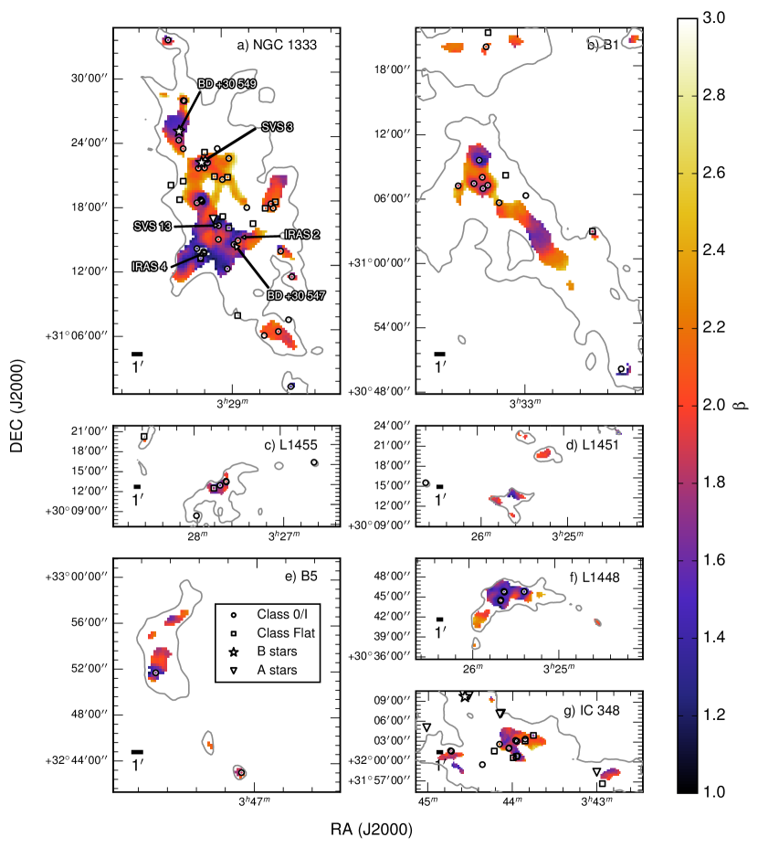
Figure 5: Derived  maps of the seven Perseus clumps, with the colors scaled linearly from 1 to 3. Symbols and contours are the same as in Figure 3.

Figure 5 shows maps of derived in the seven Perseus clumps. The 1-$\sigma$ uncertainties in the  measurement due to flux calibration uncertainties are relatively independent of the derived  values and have a median value of $\sim 0.35$ in Perseus. Pixels with similar values tend to form well-defined structures, indicating that variations seen in these clumps are correlated with local environment and not noise artifacts. Interestingly, low structures tend to correlate with local $T_{d}$ peaks.

To a lesser extent, low  structures also appear to correlate with outflows traced by CO emission (e.g., see Figure 10 for details). The CO contribution to these maps has been subtracted although the percentage contamination seen in most pixels is less than the flux uncertainties of 10% with the exception of a few special, local cases (Chen 2015). The additional uncertainty on the 850 µm fluxes associated with the CO removal process is negligible. The resemblance between some of the minima and outflow structures is therefore unlikely to be an artifact due to errors in the CO decontamination. While no study of free-free emission has been conducted over these outflows to assess whether or not such emission can be a significant contaminant in our data, free-free emission at centimetre wavelengths observed in radio jets is generally $<$ 1 mJy (Anglada 1996). Free-free emission is also expected to be relatively weak at 850 µm compared to the RMS noise of our 850 µm data, given that these jets have widths much smaller than the JCMT beam. High angular resolution observations of the outflow sources SVS 13 (Rodríguez et al. 1997; Bachiller et al. 1998) and IRAS 4A (Choi et al. 2011) in NGC 1333 with the Very Large Array (VLA) have also shown that free-free emission is negligible at $\lambda\lesssim 3$ mm at these locations. The VLA survey of the Perseus protostars conducted by Tobin et al. (2016) also found free-free emission near protostars to be faint relative to sub-millimeter dust emission and very compact with respect to our convolved $36.3^{\prime\prime}$ beam. Free-free emission is therefore unlikely to contaminate our data.

Pixels with  $\geq 3$ are found only in NGC 1333, mostly on the north-western edge where the filtering mask may be affecting the emission, as discussed in Section 4.2. Therefore, we do not trust these steep  values. Low values ($\lesssim 1.5$), however, are generally well within the filtering mask, and are likely robust against the filtering systematics.

Figure 6: Histograms of percentage of pixels with derived  values for seven Perseus clumps.

Figure 6 shows the histograms of derived values from various clumps in Perseus. Unlike $T_{d}$, the distributions of different clumps do not share a similar shape. While four clumps in Perseus appear to have a single peak (i.e., NGC 1333, IC 348, L1455, and B5), the other three clumps (i.e., B1, L1448, and L1451) appear to have two or even three peaks. The separations between most of these peaks are larger than the median  uncertainty ($\sim 0.35$), suggesting that these multiple peaks are not artifacts. The  values of the primary peak in each clump range between 1.5 (e.g., L1448) and 2.2 (e.g., B1), and the  values of most pixels range between 1.0 and 2.7. The latter range of  values is similar to that found in nearby star-forming clouds by Dupac et al. (2003; $1.0\leq$ $\leq 2.5$) and for luminous infrared galaxies by Yang & Phillips (Yang & Phillips 2007; $0.9\leq$ $\leq 2.4$).

The appearance of our derived  map of B1 is morphologically consistent with that derived by Sadavoy et al. (2013) using the same observations reduced with earlier recipes. Due to improvements in the data reduction, our derived  values are more reliable. The majority of our derived  values are lower than those derived by Sadavoy et al. by $\lesssim 0.7$, with the remaining pixels having higher values by $\lesssim 0.3$. The overall distribution of our derived  is shifted downwards by $\sim 0.2$ relative to that of Sadavoy et al., with the primary peak being skewed towards the higher end of the distribution instead of the lower end.

Figure 7 shows maps of derived $\tau_{300}$ in the seven Perseus clumps, overlaid with the same symbols as Figures 3 and 5. Column densities can be further derived from $\tau_{300}$ using Equation 2 by assuming a $\kappa_{\nu_{0}}$ value. The median uncertainty in the $\tau_{300}$ measurement derived from the covariance of the fit with $T_{d}$ and  fixed at the best determined values is $\sim 1.5\%$. The typical uncertainties due to flux calibration uncertainties, however, as seen in the Monte Carlo simulation, is about a factor of 2 (see Appendix A). Higher $\tau_{300}$ structures seen in the B1, IC 348, L1448, and NGC 1333 clumps are found along filamentary structures, much like their dust emission counterparts. This similarity is less clear in the B5, L1455, and L1451 clumps where the areas where SEDs were fit (SNR $>10$) are relatively small.

Embedded YSOs are preferentially found towards local $\tau_{300}$ peaks. Many of these embedded YSOs, however, are spatially offset from the center of these peaks, often by slightly more than a beamwidth of our maps. The differences between  values found between these offsets are smaller than those expected from the anti-correlated uncertainties discussed in Appendix A. Interestingly, we did not find any embedded YSOs towards the centers of the highest $\tau_{300}$ peaks in all Perseus clumps, with the exception of IC 348, which does not have $\tau_{300}$ peaks with distinct high values. The $T_{d}$ values of these starless $\tau_{300}$ peaks are also much lower than their surroundings, suggesting that these structures are cores well shielded from the interstellar radiation field (ISRF) due to their high column densities.

Table 3: Derived column densities in Perseus clumps

Clump	$\overline{N}\left(H_{2}\right)$	$\sigma_{N\left(H_{2}\right)}$	Number of pixels
B5	1.0	0.54	120
IC 348	1.4	1.0	537
B1	2.4	1.8	616
NGC 1333	1.9	1.7	1362
L1455	1.2	0.59	119
L1448	2.0	1.3	449
L1451	0.78	0.31	158

Note. — The units of mean and standard deviation of column densities, $N(H_{2})$, are both $10^{22}$ cm^-2.

The $T_{d}$ values near embedded YSOs and towards higher $\tau_{300}$ regions also tend to be lower than in the lower $\tau_{300}$ regions, suggesting that protostellar heated regions can appear cooler due to being more deeply embedded and having more cool dust along the line of sight. Table 3 shows the mean column densities found in each of the Perseus clumps. Indeed, the clumps with significant amounts of cold ($\lesssim 13$ K) pixels near embedded YSOs, i.e., B1, NGC 1333, and IC 348, have the first, third, and fourth highest mean column densities in Perseus, respectively. The B1 clump in particular has the majority of its pixels near embedded YSOs at $\lesssim 13$ K.

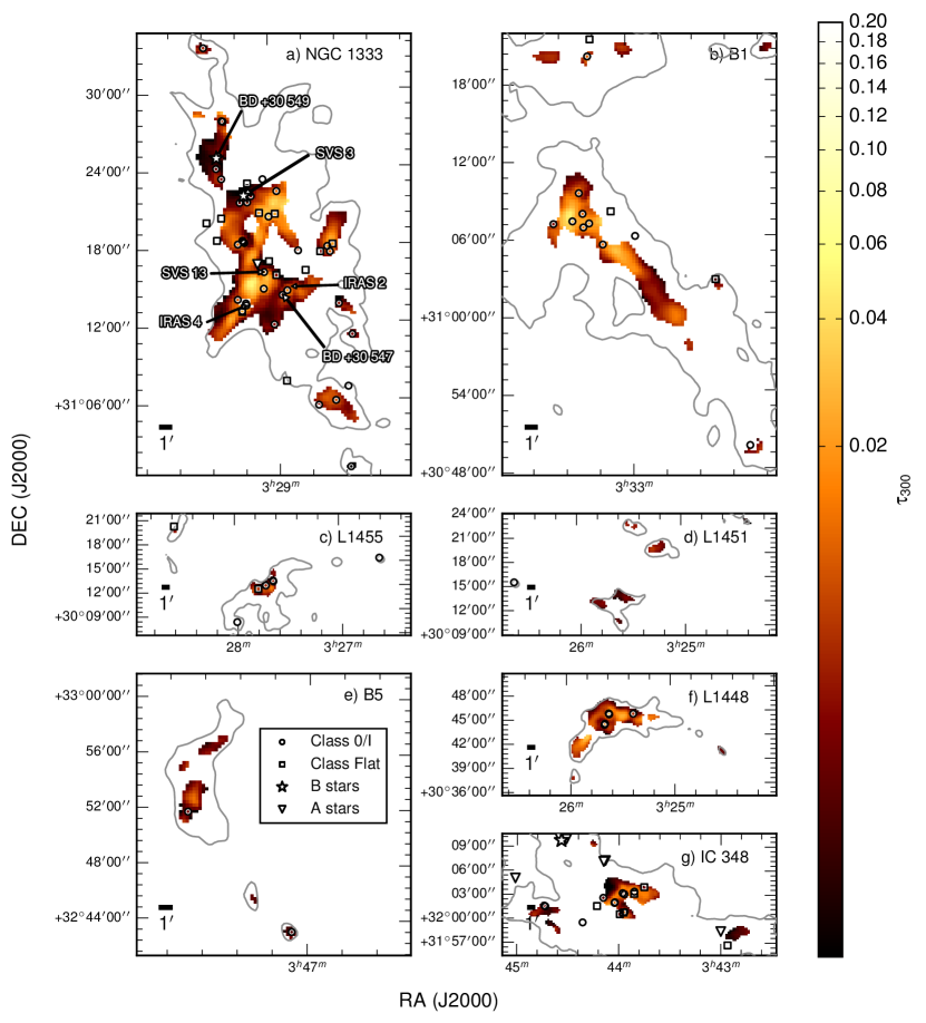
Figure 7: Derived $\tau_{300}$ maps of the seven Perseus clumps, with the colors scaled logarithmically from 0.0035 to 0.1. Symbols and contours are the same as in Figure 3.

4.4 The , $T_{d}$, and $\tau_{300}$ Relations

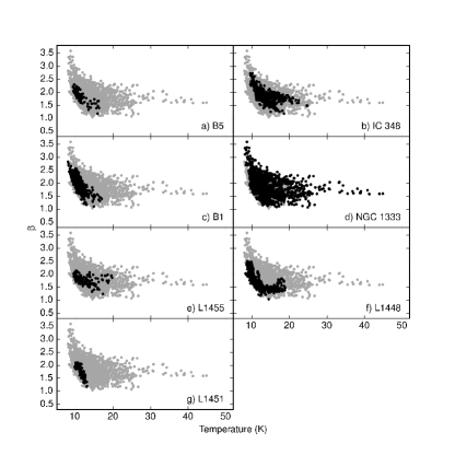
Figure 8: Scatter plots of derived vs. $T_{d}$ for each Perseus clump (black) overlaid onto the same for all Perseus clumps combined (grey).

Figure 8 shows scatter plots of  versus $T_{d}$ for all seven Perseus clumps. At $T_{d}\lesssim 16$ K, anti-correlations between and $T_{d}$ are found in all cases and cannot solely be accounted for by the anti-correlated - $T_{d}$ uncertainties discussed in Appendix A. At these $T_{d}$ values, there appears to be a prominent population of pixels in all seven clumps that exhibits a fairly linear relationship with a slope of $\sim-0.3$. Three clumps in particular, B1, B5, and L1451, seem to consist only of this population. While this slope is similar to those found in the anti-correlated uncertainties presented in Appendix A (see Figure 14), the range of  found in this population is greater than the calculated  uncertainties.

The other four Perseus clumps contain additional populations that extend into warmer temperatures ($T_{d}\gtrsim 16$ K) and have slopes which are much shallower than $-0.3$. In particular, the second population found in L1448 at $T_{d}\gtrsim 13.5$ K appears to have a constant  value of $\sim 1.4$ with a spread of $\pm\sim 0.15$. This spread in  is smaller than the estimated uncertainties based on the assumed absolute flux calibration error, which is systematic across a map. This result suggests that our relative, pixel-to-pixel uncertainties within a map are indeed relatively small, and further indicates that there indeed is an underlying anti-correlation between  and $T_{d}$. The  values found in these warmer populations are generally lower than those found at colder temperatures ($T_{d}\sim 10$ K), but are not necessarily the lowest values found within a clump.

Figure 9 shows scatter plots of derived versus $\tau_{300}$, where these appear to be weakly, postively correlated. Given the positive correlation between  and $\tau_{300}$ uncertainties discussed in Appendix A, however, we do not consider this correlation to be significant.

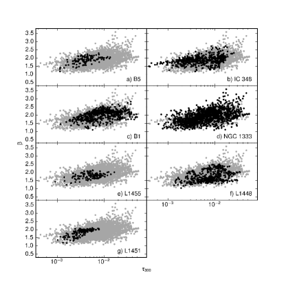
Figure 9: Scatter plots of derived vs. $\tau_{300}$ for each Perseus clump (black) overlaid onto the same for all Perseus clumps combined (grey).

5 Discussion

5.1 Radiative Heating

Throughout Perseus, we see evidence of embedded YSOs and nearby B stars heating their local environments. In contrast with the most common $T_{d}$ found in Perseus, $\sim$10.5 K, the $T_{d}$ near embedded YSOs are typically $\sim$ 14 - 20 K and can be well above 30 K near a B star where $T_{d}$ is not well constrained with our data. While not all embedded YSOs are associated with local $T_{d}$ peaks, all the local $T_{d}$ peaks coincide with locations of embedded YSOs and B stars. The only exceptions are the two extended warm regions in IC 348 that appear to be heated by sources outside of our parameter maps. Indeed, the main star cluster in IC 348 is located just northeast of the eastern warm region, while an A star is located just northeast of the western warm region. A higher local interstellar radiation field from the nearby young star cluster (Tibbs et al. 2011) likely explains why the most common $T_{d}$ found in IC 348 ($\sim$11.5 K) is slightly warmer than the other Perseus clumps.

The majority of the heated regions centered on embedded YSOs are larger than the FWHM beam of our map ($36.6^{\prime\prime}$), often having T${}_{d}\geq 15$ K out to one full beam width from the center. In NGC 1333, all the locally heated regions with radii nearly one beam width in extent coincide with at least a Class 0 or I YSO with bolometric luminosity, $L_{bol}$, of 4 L_⊙ - 33 L_⊙ (Enoch et al. 2009). In other Perseus clumps, similar regions coincide with at least a Class 0 or I YSO with bolometric luminosity of 1 L_⊙ - 5 L_⊙. If we assume our distances to the western and eastern side of Perseus to be 220 pc (Cernis 1990, Hirota et al. 2008) and 320 pc (Herbig 1998), respectively, then these heated regions would have radii of $\sim 8000$ AU and $\sim 12000$ AU, respectively, which is somewhat less than the typical size of a dense core ($\sim$15000 AU in radius, André et al. 2000).

The core $T_{d}$ profile due to protostellar heating can be modelled with radiative transfer codes. Using Dusty (Ivezic et al. 1999), Jørgensen et al. (2006) modelled such $T_{d}$ profiles for various core density profiles, protostellar bolometric luminosities, and interstellar radiation fields (ISRF), assuming the OH5 dust opacities (Ossenkopf & Henning 1994). For a core modelled after the MMS9 core in the Orion molecular cloud with density profile of $n=n_{0}(r/r_{0})^{-1.5}$, where $r_{0}=50$ AU and $n_{0}=2.7\times 10^{8}$ cm^-3, its $T_{d}$ drops down to 15 K at a radius of 2000 AU when an ISRF based on the solar neighborhood value (i.e., the standard ISRF) and a L${}_{bol}=$ 10 L_⊙ for the central source are assumed. Despite having assumed an L_bol that is relatively high, the size of this local heating is a factor of 4-6 smaller than what we find in Perseus. Given that the angular size of this modelled $T_{d}$ profile is smaller than our beam, further analysis that takes beam convolution and its associated errors into account will be needed to make a definitive comparison between the observed $T_{d}$ profile and the model.

Regions locally heated by B stars are more extended than regions heated by protostars. In NGC 1333, we find regions heated by B stars to be $\sim 1.6^{\prime}$ in radius, corresponding to $\sim$ 21000 AU. Since these B stars are not embedded objects, the temperature profile of their surrounding dust can be reasonably approximated in the optically thin limit. An analytic expression of such a temperature profile first derived by Scoville & Kwan (1976) can be generalized as

$$T_{d}(r)=50Q_{abs}^{-q/2}\left(\frac{r}{2\times 10^{15}\textup{m}}\right)^{-q}\left(\frac{L_{bol}}{10^{5}\textup{L}_{\odot}}\right)\textup{K}$$ (3)

where $Q_{abs}$ is the absorption efficient of a dust grain at $\lambda=50$ µm, and $q=2/(4+\beta)$ (Equation 1, Chandler et al. 1998). For the expected range of  values between 1 and 2, the $q$ parameter does not vary significantly. The power-law slopes of the temperature profile at these  values resemble the Dusty profile of Jørgensen et al. (2006) at larger radii where the protostellar envelope is expected to be optically thin, before the ISRF heating starts to become dominant.

We modelled the radial temperature profiles near the two B stars in NGC 1333 by assuming $\beta=1.6$, the typical $\beta$ found near these two B stars, and normalizing Equation 3 to Wolfire & Churchwell’s (1994) dust emission models with $Q_{abs}^{-q/2}=1.2$, as Chandler et al. (1998; 2000) and Jørgensen et al. (2006) did. Given that the B stars BD +30 549 and SVS 3 have luminosities of 42 L_⊙ (Jennings et al. 1987) and 138 L_⊙ (Connelley et al. 2008), respectively, the temperatures of these two stars are expected to drop down to 15 K at radii of $\sim$13000 AU and 24000 AU, comparable to the projected distances of 21000 AU (i.e., $\sim 1.6^{\prime}$) that we observed.

The localized, radiative heating due to YSOs and B stars may provide star-forming structures with additional pressure support. When treating a star-forming structure as a body of isothermal ideal gas with uniform density, the smallest length at which such an object can become gravitationally unstable due to perturbation, i.e., the Jeans length ($\lambda_{J}$), is related to the object’s temperature by $\lambda_{J}\propto T^{1/2}$. The total mass enclosed within a Jeans length, i.e., the Jeans mass ($M_{J}$), scales as $M_{J}\propto T^{3/2}$.

Even though protostellar heating is the most common form of local heating observed in Perseus, protostellar cores are likely no longer Jeans stable given that they are currently collapsing into protostars. Protostellar heating could also provide additional Jeans stability to inter-core gas, but none of the warm regions in Perseus heated by solar-mass YSOs extends beyond the typical radius of a core ($\lesssim$ 15000 AU, André et al. 2000).

While B stars are unlikely to have circumstellar envelopes themselves, they may be capable of heating nearby protostellar cores. Indeed, three SCUBA cores identified by Hatchell et al. (2005) are located in projection within these B-star heated regions: HRF57, HRF56, and HRF54. These cores do not contain known YSOs and have beam averaged $T_{d}$ between 19 K and 40 K. If we assume the densities of these cores remain unchanged in the process of heating and the gas in these cores are thermally coupled to the dust, then the associated Jeans masses of these cores at their respective temperatures are a factor of $\sim$ 3 - 8 higher than those of their counterparts at 10 K.

5.2 Outflow Feedback

Several studies of dust continuum emission in NGC 1333 (Lefloch et al. 1998; Sandell & Knee 2001; Quillen et al. 2005), as well as other nearby star-forming clumps (e.g., Moriarty-Schieven et al. 2006), have suggested that outflows play a significant role in shaping the local structure of star-forming clumps. Indeed, kinematic studies of outflows in Perseus (e.g., Arce et al. 2010; Plunkett et al. 2013) showed that outflows can inject a significant amount of momentum and kinetic energy into their immediate surroundings. As with these prior dust continuum studies, we find several $\tau_{300}$ cavities that coincide with bipolar outflows, particularly towards the ends of outflow lobes, in NGC 1333 and L1448 (see Figures 10). Due to warmer $T_{d}$ values, which can cause low column density dust to emit brightly, some of these cavities were not revealed directly by single-wavelength continuum emission alone.

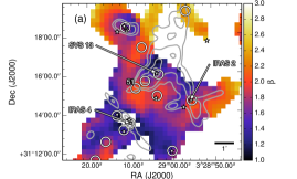
(a)

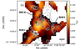
(b)

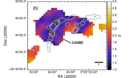
(c)

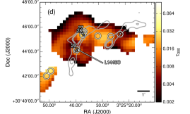
(d)

Figure 10: Maps of derived  in a) NGC 1333 and b) L1448 and their $\tau_{300}$ counterparts c) and d), respectively. These maps are overlaid with the SCUBA cores identified by Hatchell et al. (2005; circles), Class 0/I YSOs identified by Dunham et al. (2015; stars), and contours of spatially filtered, integrated ¹²CO 3-2 emission (grey). Contours of CO emission are drawn at 15 mJy beam^-1, 30 mJy beam^-1, 80 mJy beam^-1, and 110 mJy beam^-1 for the NGC 1333 maps and at 10 mJy beam^-1, 20 mJy beam^-1, and 25 mJy beam^-1 for the L1448 maps. The colors in panels a and b are scaled linearly between 1.0 - 3.0, and logarithmically between 0.002 - 0.2 and 0.002 - 0.1 for panels c and d, respectively. Only the cores mentioned in the text are identified with numbers designated by Hatchell et al.

In addition to low $\tau_{300}$ regions, we also find two high $\tau_{300}$ regions in Perseus that may have been formed from compression by nearby outflows. For example, the high $\tau_{300}$ region near the starless core HRF51 in NGC 1333 has the highest $\tau_{300}$ values in the clump, and is also located towards the southeastern end of the outflow associated with the HH7-11 outflows driven by SVS 13 (Snell & Edwards 1981). The high $\tau_{300}$ region surrounding the HRF27 and HRF28 cores in L1448 also has the second highest $\tau_{300}$ values found in L1448, and is located on the northeastern end of the outflow originating from L1448C (HRF29, a.k.a. L1448-mm) near HH197 (e.g., Bachiller et al. 1990; Bally et al. 1997). The presence of Herbig-Haro objects in these high $\tau_{300}$ regions indicates that outflows are indeed interacting with ambient gas at these locations and perhaps compressing the gas (and dust) in the process, resulting in the observed high $\tau_{300}$ values. Given that the $\tau_{300}$ values we find around the starless core HRF51 are unusually high in comparison with the rest of Perseus, HRF51 would be a good candidate for followup observations to test the limits of starless core stability.

We do not find evidence for shock-heating from outflows in our $T_{d}$ maps, which is unsurprising given that shock heated gas is not well coupled to dust thermally (e.g., Draine et al. 1983; Hollenbach & McKee 1989). The dominant local influence of outflows appears to be their ability to reshape local structures such as cores and filaments. Indeed, gas compression driven by outflows can stimulate turbulence to form starless cores beyond simple Jeans instability. For example, the extra material being pushed towards a starless core by outflows can provide the needed perturbation to trigger core collapse, as well as providing the core with extra mass to accrete. On the other hand, these outflows can in principle also inject turbulence into the structures they compress, providing additional pressure support for these dense structures to remain temporarily stable against Jeans instability. The mechanical feedback from outflows, therefore, is likely important in regulating star formation in clustered environments where it can enhance or impede the processes through compression or clearing, respectively.

5.3 Beta and Clump Evolution

The global properties of a star-forming clump are expected to evolve significantly as star formation progresses within it. Given that dust grains can undergo growth inside cold, dense environments and potentially be fragmented or destroyed in energetic processes, dust grains themselves are expected to evolve over time. If grain evolution in a clump is dominated by processes that result in a net change in , such as growth in maximum grain sizes (Testi et al. 2014), then we should be able to observe the global values of  varying from clump to clump due to the different evolutionary stages of these clumps.

5.3.1 Beta Variation and its Relation to Temperature

In Perseus, we find significant  variations within individual clumps. As shown in Figure 6, the majority of values in these clumps range from 1.0 to 2.7. The spatial distribution of  is not erratic, and appears fairly structured on a local scale, suggesting that is likely dependent on the properties of the local environment. Furthermore, the spatial transition between pixels with $>2$ and $<1.6$, though relatively sharp, is not abrupt with respect to our beam width ($36.3^{\prime\prime}$ FWHM). The overall appearance of the  structures, as well as their $T_{d}$ and $\tau_{300}$ counterparts, is fairly smooth and coherent on scales larger than the beam, suggesting that our derived  values are robust against random noise.

In Figure 8, our derived and $T_{d}$ values appear to be anti-correlated, similar to behavior found in prior studies of nearby star-forming regions at lower angular resolutions (e.g., Dupac et al. 2003; Planck Collaboration et al. 2011). As detailed in Appendix A, this anti-correlation cannot be solely accounted for by the anti-correlated  - $T_{d}$ uncertainties associated with our SED fits. The fact that lower  regions tend to be spatially well structured and coincide with locations that are locally heated by known stellar sources further demonstrates that there indeed exists an anti-correlation between  and $T_{d}$ that is not an artifact of the noise.

Shetty et al. (2009b) have shown that line-of-sight $T_{d}$ variations can lead to an underestimation of and an overestimation of density-weighted $T_{d}$ (column temperature) by fitting a single-component modified blackbody curve to the SEDs of various models of cold cores and warm envelopes that have a single value. When these synthetic SEDs are noiseless and are equally well sampled in both the Wien’s and Rayleigh-Jeans’ regimes, Shetty et al. found that systematic exclusion of shorter wavelength data, i.e., the bands toward the Wien’s regime, will allow the  and $T_{d}$ values drawn from fits to approach the true  values and column temperatures. A single-component modified blackbody curve simply does not fit well SEDs with multiple temperature components in the Wien’s regime.

In Perseus, we find the median $T_{d}$ of starless cores to be $9.8$ K when cores in IC 348 are excluded. The median $T_{d}$ of starless cores in IC 348 is a bit higher ($11.7$ K), likely due the clump having a higher ISRF. The former $T_{d}$ is consistent with both the typical core $T_{d}$ found by Evans et al. (2001; $\sim 10$ K) and the modelled column temperature of 9.6 K from Shetty et al. (2009b), which was itself based on the core density and $T_{d}$ profiles of Evans et al. The agreement between our derived $T_{d}$ and Shetty et al.’s modelled column temperature suggests that our fits to the SEDs of these cold cores are robust against line-of-sight $T_{d}$ variation. If the true  values along the lines of sight of our observations are fairly uniform, then our derived  values should approach those of the true , as demonstrated by Shetty et al. Figure 11a shows a typical example of an SED found in cold core that is well fit by a single component modified blackbody curve.

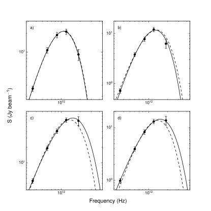
Figure 11: Best SED fits to four selected pixels in NGC 1333 with $T_{d}$, , and $\tau_{300}$ as free parameters (solid), and with  fixed at a value of 2 (dash). The best fit $T_{d}$ values in panels a, b, c, and d with  as a free parameter are 10.6 K, 11.4 K, 16.3 K, and 16.8 K, respectively. Their corresponding best fit  values are 2.0, 2.4, 1.6, and 1.4, respectively. The error bars represent the flux calibration uncertainties in each bands (i.e., 20% for the SPIRE 160 µm band and 10% for the other bands).

In warmer regions, some of our SED fits have trouble reconciling the shortest wavelength band (i.e., 160 µm), suggesting that line-of-sight $T_{d}$ variation may be a concern in these specific regions. Figures 11b-d show some examples. Given that preferential sampling towards the Rayleigh-Jeans tail will allow SED fits to place a tighter constraint on , as Shetty et al. demonstrated, the  values we measured across 160 - 850 µm toward the warmer regions should remain fairly robust against $T_{d}$ variation along the line of sight as the peaks of these SEDs shift further toward shorter wavelengths. Indeed, the fact that our sampled SED fits only have trouble fitting the 160 µm bands in warmer regions suggests that these SED fits are preferentially anchored towards the longer wavelength points where  can be more robustly determined. Measurements of the flux ratio between the longer wavelength bands in NGC 1333 by Hatchell et al. (2013; SCUBA-2 450 µm and 850 µm bands) and in Perseus by Chen (2015; SPIRE 500 µm and SCUBA-2 850 µm bands) have further confirmed that these regions are indeed warm and the $T_{d}$ drawn from the SED fits are not erroneous due to poor fits to the shorter wavelength bands.

5.3.2 The Cause Behind  Variations

The  value of a grain population depends on various physical properties of its grains. The  value we derived in a given pixel should therefore be viewed as an effective  of the various underlying populations seen along the line of sight. If these effective  values are dominated by the  of a single grain population, then a simple comparison with laboratory measurements may reveal some physical properties of this particular population.

Laboratory measurements have shown that values can be intrinsically temperature dependent (e.g., Agladze et al. 1996; Mennella et al. 1998; Boudet et al. 2005). Many of these measured dependencies, however, are not significant enough to explain by themselves the anti-correlation seen here. Agladze et al. (1996) found two species of amorphous grains with values that decrease from $\sim$ 2.5 to $\sim$ 1.7 - 2 as the $T_{d}$ increases from 10 K to 25 K. While these measured temperature dependencies are not strong enough to be the sole cause of the anti-correlation seen here, they are perhaps significant enough to provide a partial contribution.

Dust coagulation models have shown that grain growth can cause values to decrease significantly from the typical diffuse ISM value ( $\sim$ 2), to as low as zero (e.g., Miyake & Nakagawa 1993; Henning et al. 1995). Since dust coagulation is favored in a denser environment, where the dust collision rates are higher, lower values may be expected towards the densest regions.

As shown in Figure 9, we do not find evidence that is anti-correlated with $\tau_{300}$, and thus column density. In contrast, we find that the highest $\tau_{300}$ structures in Perseus tend to have $\gtrsim 2$, especially towards the colder regions not associated with localized heating. The lack of decrease in towards these dense regions, however, is not sufficient to rule out grain growth through coagulation. The presence of ice mantles on the surface of dust grains, for example, can increase the  value from that of bare grains, i.e., $\sim 2$, to $\sim 3$ for dust typically found in diffuse ISM (Aannestad 1975) and from $\sim 1$ to $\sim 2$ for modelled dust in the densest star-forming environments (Ossenkopf & Henning 1994). Since the growth of ice mantles is also favored in the coldest and densest environments, such growth can, in principle, compete with coagulated grain growth by modifying in opposite directions, causing the dust in some of the highest $\tau_{300}$ regions to have $\sim 2$ instead of higher or lower values.

Given that the presence of ice mantles on grain surfaces may be capable of suppressing the decrease in caused by coagulated grain growth, we speculate that the - $T_{d}$ anti-correlation may be explained by the sublimation of ice mantles in warmer environments. This hypothesis is useful in explaining why internally heated protostellar cores have lower values than their starless, non-heated counterparts. Measuring the depletion levels of molecules of which ice mantles typically composed of towards heated and non-heated cores could test this hypothesis, provided these molecules can themselves survive in these heated environments.

While lower  regions tend to coincide with locally heated regions, these  regions also tend to be more spatially extended than the heated regions. The low- region surrounding IRAS 4 in NGC 1333 is a prominent example of this behavior. Interestingly, many low regions also coincide with the locations of bipolar outflows, prompting us to suspect that outflows may be capable of carrying lower grains from deep within a protostellar core out to a scale large enough to be observed with our spatial resolution. Recent high resolution, interferometric studies on the inner regions of a small number of protostellar envelopes have found that  $\leq 1$ (Chiang et al. 2012; Miotello et al. 2014), suggesting that dense, inner regions of cores may indeed be a site for significant grain growth. Further high angular resolution observations of within protostellar and prestellar cores may verify if low grains are preferentially found deep within a dense core, and whether or not their production is associated with the presence of protostars or disks.

Interestingly, the dependence of  on the maximum grain size, $a_{max}$, assuming a power-law grain size distribution, i.e., $n(a)\propto a^{-q}$, behaves similarly regardless of other  dependencies (Testi et al. 2014; see their Figure 4). When $a_{max}$ is less than $\sim 10$ µm, the  values computed by Testi et al. are all between $\sim$ 1.6 - 1.7, independent of the dust grain’s chemical composition and porosity. As $a_{max}$ increases,  values for all three models first increase upwards to a maximum value of $\sim 2.5$ for compact grains, or $\sim 2$ for porous icy grains, and then quickly drop down to values less than 1 starting at $a_{max}\gtrsim 10^{3}$ µm. The  values computed by Testi et al. are for wavelengths measured between 880 - 9000 µm, which do not overlap with our observed wavelengths between 160 - 850 µm. Nevertheless, given that a dust grain has less accessible modes to emit photons with wavelengths longer than or comparable to its physical size, we expect the same  dependency on $a_{max}$ to hold in our observed wavelength range with the corresponding $a_{max}$ shifted towards smaller values. Complementary  measurements at wavelengths greater than 850 µm will test this idea.

If we assume the  dependency on $a_{max}$ to be the dominant, global driver of  evolution in a clump, as shown by Testi et al. (2014), while the other  dependencies are only locally significant, then  values observed on the global scale of a clump should be a good proxy to measure the relative evolutionary stage of a clump in terms grain growth.

5.3.3 Beta Variations Between Clumps

As demonstrated in Figure 6, the  distributions in Perseus differ significantly from clump to clump, suggesting that the dust grains are co-evolving with their host clumps. To make the measurement of  variation more sensitive, we binned our  values into three categories, with  values of 1.5 - 2, 2 - 3, and 0 - 1.5 to represent pristine, transitional, and evolved values of $a_{max}$, and thus , respectively. This choice is based on Testi et al’s (2014) modelled  - $a_{max}$ relations, and we extended the upper limit of the pristine, i.e., medium,  bin to a value of 2 to include the observed  values of $\sim 2$ in the diffuse ISM. While  values of dust do go through the “pristine” category again as they migrate from the transition category to the evolved category, this typically only occurs over a very narrow range of $a_{max}$ values relative to the overall $a_{max}$ values considered. To quantify the advancement of grain growth in each clump, we devise the growth index, $G$, as follows:

$$G=100-P_{pri}+P_{evo}$$ (4)

where $P_{pri}$ and $P_{evo}$ are the percentage of pixels in each clump with the pristine and evolved values, respectively. As the typical $a_{max}$ in a clump increases, the $100-P_{pri}$ term increases as  migrates away from the pristine values, resulting in an increase in $G$. When the grain growth enters an advanced stage, the increase in $a_{max}$ will also increase the value of $P_{evo}$, resulting in further increase in $G$.

Figure 12: Bar graph of derived  in the seven Perseus clumps binned to the three categories based on calculations by Testi et al. (2014): pristine (P), transitional (T), and evolved (E). The corresponding  values in these three categories are 1.5 - 2, 2 - 3, and 0 - 1.5, respectively. The order of the clumps are rearranged here from the least evolved to the most evolved as suggested by growth index, $G$, defined in Equation 4 and shown here in each panel.

Figure 12 shows the percentage of pixels in each of the  categories for the seven Perseus clumps and their corresponding $G$ values. The  bins are arranged in the order of pristine, transitional, and evolved categories from left to right. The order of the clumps here has been rearranged in the order of increasing $G$, corresponding to the perceived increase in $a_{max}$ based on calculations by Testi et al. (2014). As seen in Figure 12, the dust population in each of the Perseus clumps appears to be in a different evolutionary stage. For a reference, the median  uncertainty is $\sim 0.35$. In terms of their relative dust evolution, the Perseus clumps are ordered as L1455, L1451, IC 348, B5, B1, NGC 1333, and L1448. We note that our sample sizes vary significantly from clump to clump, ranging from 1362 pixels in NGC 1333 to only 119 pixels in L1455. Our ability to make comparison between clumps is therefore limited by these sample size differences and the associated uncertainties in measuring .

It may seem surprising at first that the measured  values would suggest IC 348 to be a less-evolved clump in Perseus, given that IC 348 has often been considered to be an older star-forming clump near the end of its star-forming phase (Bally et al. 2008). The region covered by our SED fits, however, actually traces a filamentary ridge of higher density gas just southwest of the main optical cluster. This sub-region hosts a higher fraction of Class 0 and I YSOs and a lower fraction of Class II and III YSOs relative to the rest of IC 348 (Herbst 2008). The relatively higher abundance of embedded YSOs in comparison to their more-evolved counterparts in this area of IC 348 suggests that this sub-region is indeed quite young. Due to low number statistics ($\leq 10$ YSOs), we did not perform a similar consistency check on the youngest clumps, L1455 and L1451.

L1448, NGC 1333, and B1 are likely the more-evolved clumps in Perseus based on their $G$ values. Indeed, the higher fractions of Class II and III YSOs relative to Class 0, I, and Flat YSOs seen in NGC 1333 (Sadavoy 2013) suggest that NGC 1333 is one of the most evolved clumps in Perseus. Interestingly, B1 has the highest fraction of transitional  values and the lowest fraction of evolved  values in Perseus. Given that B1 also has the highest mean column density in Perseus (see Table 3), B1 may potentially be a younger clump with an enhanced grain-growth due to its higher density.

In general, we do not expect the fraction of embedded YSOs and the relative dust evolutionary state to be tightly correlated given that the fraction of embedded YSOs is more indicative of the current star-forming rate whereas the dust evolutionary state measures the accumulated grain growth throughout a clump’s history. Considering that grain growth is subjected to factors such as density and temperature over time, which may also differ between clumps, we do not expect the relative evolution we inferred from $a_{max}$ to be strictly proportional to time either.

As mentioned in Section 4.4, we find a significant anti-correlation between  and $T_{d}$ in all seven Perseus clumps that cannot be solely accounted for by the anti-correlated uncertainties driven by noise or $T_{d}$ variation along the line of sight. Interestingly, there appears to be a population of pixels in all seven clumps that are located at the bottom left corner of the - $T_{d}$ scatter plots with $T_{d}$ less than 20 K (see Fig. 8). The anti-correlation displayed by this particular population appears fairly linear, and has a slope of $\sim-0.3$. This population is primarily responsible for the wide range of values observed in each clump and its presence in all seven clumps may suggest a universal dust evolution that is common to all star-forming clumps. The  - $\tau_{300}$ distributions of Perseus clumps (see Fig. 9) all behave fairly similarly and do not show obvious trends associated with clump evolution.

6 Conclusion

In this study, we fit modified blackbody SEDs to combined Herschel and JCMT continuum observations of star-forming clumps in the Perseus molecular cloud and simultaneously derived dust temperature, $T_{d}$, spectral emissivity index, , and optical depth at 300 µm, $\tau_{300}$, using the technique developed by Sadavoy et al. (2013). We performed a detailed analysis of the derived $T_{d}$, , and $\tau_{300}$ values in seven Perseus clumps, i.e., B5, IC 348, B1, NGC 1333, L1455, L1448, and L1451, and investigated anti-correlated uncertainties between  and $T_{d}$. We found that the  - $T_{d}$ anti-correlations seen in Perseus are significant and are not artifacts of noise or calibration errors. In addition, we demonstrated that our final SED fits are robust against systematic uncertainties associated with temperature variation along lines-of-sight.

We summarize our main findings as follows:

1. The most common (i.e., mode) $T_{d}$ seen in Perseus clumps is $\sim 10.5$ K, except in IC 348 where it is $\sim 11.5$ K. The former $T_{d}$ is consistent with the kinetic temperatures of dense cores observed with ammonia emission lines in Perseus ($\sim$11 K; Rosolowsky et al. 2008; Schnee et al. 2009), and the isothermal $T_{d}$ of prestellar cores seen in various clouds ($\sim$10 K; Evans et al. 2001). The IC 348 clump being slightly warmer than the rest of Perseus may be due to stellar heating from the nearby young star cluster.

2. Nearly all the local $T_{d}$ peaks found in Perseus coincide with locations of embedded YSOs (and nearby B stars in the case of NGC 1333), which indicates local heating by these YSOs. The immediate region surrounding an embedded YSO can have $T_{d}$ of up to $\sim 20$ K whereas that near a B star can have $T_{d}$ well above $\sim 30$ K.

3. We found significant variations over individual star-forming clumps. Most  values found in Perseus are in the range of $1.0\lesssim$ $\lesssim 2.7$, similar to that found in nearby star-forming clouds by Dupac et al. (2003; $1.0\leq$ $\leq 2.5$) and for luminous infrared galaxies by Yang & Phillips (2007; $0.9\leq$ $\leq 2.4$). Maps of , in general, appear well structured on a local scale, indicating that is likely a function of its local environment.

4. We found and $T_{d}$ to be anti-correlated in all Perseus clumps, and that lower regions tend to coincide with local $T_{d}$ peaks. These anti-correlations cannot be solely accounted for by anti-correlated and $T_{d}$ uncertainties associated with our SED fitting. The dust grains’ intrinsic dependency on temperature (e.g., Agladze et al. 1996) may be partially responsible for the anti-correlation, but is not strong enough to be the sole cause. The sublimation of surface ice mantles, which can increase when present on a dust grain (e.g., Aannestad 1975; Ossenkopf & Henning 1994), may provide an explanation for the observed anti-correlation.

5. Similar to prior studies (e.g., Sandell & Knee 2001), we found cavities and peaks in maps of derived $\tau_{300}$, and thus column density, that coincide with the ends of some outflow lobes, suggesting that these structures were cleared out or compressed by local outflows, respectively. The fact that Herbig-Haro objects were found in locations where outflows meet the highest column density structures in individual clumps further supports this view. Creating column density maps from fitting SEDs with $T_{d}$, , and $\tau$, is important for this analysis.

6. The distribution found in Perseus differs from one clump to another (see Figure 6). Binning  values into pristine (medium), transitional (high), and evolved (low) values of  as a function of maximum grain size, $a_{max}$, calculated by Testi et al. (2014) revealed that the typical $a_{max}$ value may also differ from clump to clump (see Figure 12). This result suggests that dust grains can grow significantly as a clump itself evolves.

Following Sadavoy et al. (2013), we mapped values over several star-forming clump at angular resolutions of $\sim 0.5$ arcminutes. Our study is the first of its kind to extend such analysis to the major star-forming clumps across a molecular cloud. In Perseus, we found  values which are significantly different from the diffuse ISM values (i.e., $\sim 2$), indicative of dust grain evolution in the denser, star-forming ISM. The discovery of coherent small-scale, low- regions, and their coincidence with local temperature peaks have provided some hints on the origins of these low- value grains. Further high-resolution observations of toward protostellar cores and starless cores would be most welcome. Observations of potential sublimation of ice mantles may also help to constrain the role of ice mantles.

Appendix A Anti-correlated  - $T_{d}$ Uncertainties

Anti-correlation between and $T_{d}$ can be an artifact of SED fitting using the minimization of $\chi^{2}$ method due to - $T_{d}$ degeneracy. Indeed, Shetty et al. (2009a; 2009b) demonstrated that SED fitting using the minimization of $\chi^{2}$ method can lead to such an anti-correlation when modest amounts of noise are present in data. Such anti-correlations due to erroneous fittings have also been noted in previous works (e.g., Keene et al. 1980; Blain et al. 2003; Sajina et al. 2006; Kelly et al. 2012; Sadavoy et al. 2013).

The anti-correlated  - $T_{d}$ uncertainties arise naturally from both and $T_{d}$’s ability to shift the peak of a modified blackbody SED (see Equation 1). While  is responsible for producing the power-law slope of the Rayleigh-Jeans tail of an SED, it can also shift the SED peak independent of $T_{d}$. An underestimation of , for example, leads to a shallower power-law tail that pulls the SED peak lower in frequency. $T_{d}$, on the other hand, shifts the SED peak through Wien’s displacement law, which acts on the blackbody component of the SED. The position of the SED peak can thus be maintained at a constant value by anti-correlating  and $T_{d}$, resulting in a degeneracy in reduced $\chi^{2}$ SED fitting when the height of the SED can be arbitrary scaled by a free $\tau$ parameter.

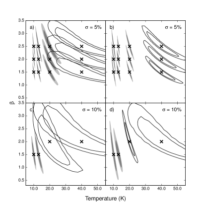
Figure 13: The 50% and 75% probability contours of $T_{d}$ and  drawn from SED fits to noisy modified blackbody models using the Monte Carlo approach. The true $T_{d}$ and  values behind the models are marked with the “X” symbols. The modelled SEDs are sampled at 160 µm, 250 µm, 350 µm, 500 µm, and 850 µm for panels a) and c), and at 100 µm, 200 µm, 260 µm, 360 µm, and 580 µm for panels b) and d). The adopted noise levels are shown in each panel.

Figure 13 shows the 50% and 75% probability contours of $T_{d}$ and  drawn from SED fits to noisy modified blackbody models using the Monte Carlo approach with flux uncertainties of $\sigma=5\%$ and $10\%$. The true $T_{d}$ and  values behind the models are marked with the “X” symbols. The modelled SEDs are sampled at the same wavelengths as our Herschel and JCMT bands for the fits shown in panels a) and c), and at the wavelengths used by Shetty et al. (2009a, i.e., 100 µm, 200 µm, 260 µm, 360 µm, and 580 µm) based on observations made by Dupac et al. (2003) for the fits shown in panels b) and d). Consistent with the results of Shetty et al. (2009a), anti-correlated uncertainties between $T_{d}$ and  are significant for SED fits to these wavelengths, even when the flux noise is relatively modest ($\sigma=5\%$). These uncertainties tend to increase with temperature as the SED peak shifts upwards away from the sampled wavelengths. The fits to SEDs are poorly constrained at $T_{d}\gtrsim 30$ K for a noise level of $\sigma=5\%$ and at $T_{d}\gtrsim 20$ K for $\sigma=10\%$.

By having a broader wavelength coverage and a better sampling of the longer wavelengths than those used by Dupac et al. (2003), we are able to achieve smaller $T_{d}$ and  uncertainties at lower temperatures ($T_{d}\sim 10$ K; see Figure 13) at a given noise level. With 160 µm as our shortest wavelength band instead of the 100 µm used by Dupac et al., however, our uncertainties due to flux noise at higher temperatures are larger than those of Dupac et al. due to having fewer samples on the SED peak. The preferential sampling of the Rayleigh-Jeans tail of the SED instead of the peak, nevertheless, is advantageous in making SED fits more robust against temperature variation along the line of sight (Shetty et al. 2009b).

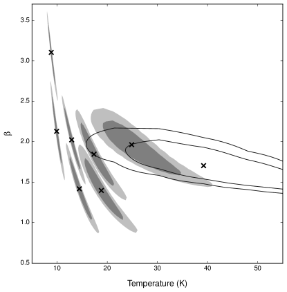
Figure 14: The 50% and 75% probability contours of $T_{d}$ and  drawn from SED fits to a few selected pixels in our NGC 1333 data using the Monte Carlo approach. The uncertainties in our data are assumed to be the dominated by flux calibration errors and random flux calibration corrections are generated for each instrument (i.e., PACS, SPIRE, and SCUBA-2) with an adopted error of 10%. The best fit $T_{d}$ and  values are marked with “X” symbols.

The median flux noises in our data over where SED fits are made are small ($<1\%$ in Herschel bands and $\sim 5\%$ in SCUBA-2 850 µm band) relative to our assumed flux calibration uncertainties ($20\%$ for PACS 160 µm band and $10\%$ for the other bands). Indeed, we found the inclusion of measured rms noise in addition to the flux calibration uncertainties (correlated within each instrument) to have a negligible effect on the $T_{d}$ and  uncertainties derived using the Monte Carlo method with the NGC 1333 data. We therefore assumed flux noise to be negligible with respect to the flux calibration uncertainties, which are systematic across a map, in our final uncertainties analysis. Due the color calibration uncertainties being of the same order as the flux noise, we also assumed the color calibration error to be negligible.

Figure 14 shows the 50% and 75% probability contours of $T_{d}$ and  drawn from SED fits to a few selected pixels in our NGC 1333 data using the Monte Carlo approach. Instead of adding random noise to each individual band, random flux calibration corrections are generated for each instrument and the bands within each instrument received the same flux correction at each iteration of the Monte Carlo simulation. We adopted a flux calibration error of 20% for PACS, 10% for SPIRE, and 10% for SCUBA-2. The best fit $T_{d}$ and  values are marked with “X” symbols. The $T_{d}$ and  uncertainties due to flux calibration we quoted in this paper are effectively derived from fitting a Gaussian to these probability contours collapsed onto one of these axises (see Sadavoy et al. 2013 for details).

As shown in Figure 14, even though the probability contours of these selected pixels collectively resemble the shape of the $T_{d}$ -  scatter plot of NGC 1333 shown in Figure 8d, the probability contours of each pixel are relatively small in comparison to the overall distribution. Furthermore, due to the flux calibration uncertainties being systematic across a map, erroneous offsets in our derived parameters should be spatially correlated on a scale of $\sim 30^{\prime}$, which is the size of our smallest maps (i.e., SCUBA-2 maps). The relative pixel to pixel uncertainties between the derived parameters in each map should therefore be smaller than the stated absolute uncertainties demonstrated in Figure 14.

The derived $T_{d}$ values are well constrained at low temperatures ($\lesssim 20$ K), which include most of our pixels (see Figure 4). At these low temperatures, the uncertainties in the derived  are relatively large with respective to the range of derived  values, and decrease only slightly at higher temperatures. Despite these large uncertainties, low, intermediate, and high  values can still be distinguished from each other at a 1-$\sigma$ confidence interval.

Our adopted flux calibration uncertainties for extended sources are relatively conservative compared to the values estimated for point sources ($<7\%$ for PACS bands, Balog et al. 2014; $\sim 5\%$ for SPIRE bands, Bendo et al. 2013; $<8\%$ for SCUBA-2 850 µm band). The most common $T_{d}$ values found in all Perseus clumps, except for IC 348, agree with each other and with the ammonia gas temperatures of Perseus dense cores (Rosolowsky et al. 2008) to within 0.5 K. In comparison, our estimated absolute $T_{d}$ uncertainties at these temperatures is $\sim 0.8$ K. This result suggests that the flux calibration uncertainties we assumed are indeed relatively conservative.

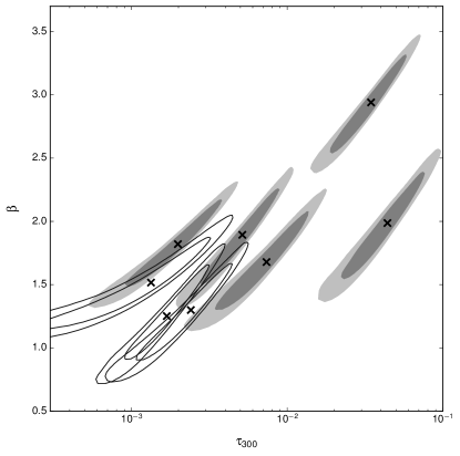
Figure 15: The 50% and 75% probability contours of $\tau_{300}$ and  drawn from SED fits to the same pixels in NGC 1333 as those in Figure 14, using the same method. The best fit $\tau_{300}$ and  values are marked with “X” symbols.

Figure 15 shows the 50% and 75% probability contours of $\tau_{300}$ and  drawn from SED fits to the same pixels as in Figure 14. As expected, $\tau_{300}$ and  are positively correlated, given that the uncertainties between $T_{d}$ and  and between $T_{d}$ and $\tau$ are anti-correlated. The anti-correlation found in the latter is due to the flux of a modified blackbody being positively correlated with $T_{d}$ (see in Equation 1). We find the slopes of the correlated uncertainties to be relatively well defined in the log($\tau$) -  space for well constrained SED fits (i.e., at $T_{d}\lesssim 30$ K), and relatively constant regardless of the fitted parameters. Given these correlated uncertainties, we did not find a significant underlying correlation between  and $\tau_{300}$ shown in Figure 9.

References

- Aannestad (1975) Aannestad, P. A. 1975, ApJ, 200, 30
- Agladze et al. (1996) Agladze, N. I., Sievers, A. J., Jones, S. A., Burlitch, J. M., & Beckwith, S. V. W. 1996, ApJ, 462, 1026
- André & Saraceno (2005) André, P., & Saraceno, P. 2005, in ESA Special Publication, Vol. 577, ESA Special Publication, ed. A. Wilson, 179–184
- André et al. (2000) André, P., Ward-Thompson, D., & Barsony, M. 2000, Protostars and Planets IV, 59
- André et al. (2010) André, P., Men’shchikov, A., Bontemps, S., et al. 2010, A&A, 518, L102
- Anglada (1996) Anglada, G. 1996, in Astronomical Society of the Pacific Conference Series, Vol. 93, Radio Emission from the Stars and the Sun, ed. A. R. Taylor & J. M. Paredes, 3–14
- Arab et al. (2012) Arab, H., Abergel, A., Habart, E., et al. 2012, A&A, 541, A19
- Arce et al. (2010) Arce, H. G., Borkin, M. A., Goodman, A. A., Pineda, J. E., & Halle, M. W. 2010, ApJ, 715, 1170
- Aspin (2003) Aspin, C. 2003, AJ, 125, 1480
- Astropy Collaboration et al. (2013) Astropy Collaboration, Robitaille, T. P., Tollerud, E. J., et al. 2013, A&A, 558, A33
- Bachiller et al. (1998) Bachiller, R., Guilloteau, S., Gueth, F., et al. 1998, A&A, 339, L49
- Bachiller et al. (1990) Bachiller, R., Martin-Pintado, J., Tafalla, M., Cernicharo, J., & Lazareff, B. 1990, A&A, 231, 174
- Bally et al. (1997) Bally, J., Devine, D., Alten, V., & Sutherland, R. S. 1997, ApJ, 478, 603
- Bally et al. (2008) Bally, J., Walawender, J., Johnstone, D., Kirk, H., & Goodman, A. 2008, The Perseus Cloud, ed. B. Reipurth, 308
- Balog et al. (2014) Balog, Z., Müller, T., Nielbock, M., et al. 2014, Experimental Astronomy, 37, 129
- Beckwith & Sargent (1991) Beckwith, S. V. W., & Sargent, A. I. 1991, ApJ, 381, 250
- Bendo et al. (2013) Bendo, G. J., Griffin, M. J., Bock, J. J., et al. 2013, MNRAS, 433, 3062
- Bintley et al. (2014) Bintley, D., Holland, W. S., MacIntosh, M. J., et al. 2014, in Proc. SPIE, Vol. 9153, Millimeter, Submillimeter, and Far-Infrared Detectors and Instrumentation for Astronomy VII, 915303
- Blain et al. (2003) Blain, A. W., Barnard, V. E., & Chapman, S. C. 2003, MNRAS, 338, 733
- Boudet et al. (2005) Boudet, N., Mutschke, H., Nayral, C., et al. 2005, ApJ, 633, 272
- Buckle et al. (2009) Buckle, J. V., Hills, R. E., Smith, H., et al. 2009, MNRAS, 399, 1026
- Cernis (1990) Cernis, K. 1990, Ap&SS, 166, 315
- Chandler et al. (1998) Chandler, C. J., Barsony, M., & Moore, T. J. T. 1998, MNRAS, 299, 789
- Chandler & Richer (2000) Chandler, C. J., & Richer, J. S. 2000, ApJ, 530, 851
- Chapin et al. (2013) Chapin, E. L., Berry, D. S., Gibb, A. G., et al. 2013, MNRAS, 430, 2545
- Chen (2015) Chen, M. C. 2015, Master’s thesis, University of Victoria
- Chiang et al. (2012) Chiang, H.-F., Looney, L. W., & Tobin, J. J. 2012, ApJ, 756, 168
- Choi et al. (2011) Choi, M., Kang, M., Tatematsu, K., Lee, J.-E., & Park, G. 2011, PASJ, 63, 1281
- Connelley et al. (2008) Connelley, M. S., Reipurth, B., & Tokunaga, A. T. 2008, AJ, 135, 2496
- Currie et al. (2014) Currie, M. J., Berry, D. S., Jenness, T., et al. 2014, in Astronomical Society of the Pacific Conference Series, Vol. 485, Astronomical Data Analysis Software and Systems XXIII, ed. N. Manset & P. Forshay, 391
- Drabek et al. (2012) Drabek, E., Hatchell, J., Friberg, P., et al. 2012, MNRAS, 426, 23
- Draine & Lee (1984) Draine, B. T., & Lee, H. M. 1984, ApJ, 285, 89
- Draine et al. (1983) Draine, B. T., Roberge, W. G., & Dalgarno, A. 1983, ApJ, 264, 485
- Dunham et al. (2015) Dunham, M. M., Allen, L. E., Evans, II, N. J., et al. 2015, ApJS, 220, 11
- Dupac et al. (2003) Dupac, X., Bernard, J.-P., Boudet, N., et al. 2003, A&A, 404, L11
- Enoch et al. (2009) Enoch, M. L., Evans, II, N. J., Sargent, A. I., & Glenn, J. 2009, ApJ, 692, 973
- Evans et al. (2001) Evans, II, N. J., Rawlings, J. M. C., Shirley, Y. L., & Mundy, L. G. 2001, ApJ, 557, 193
- Friesen et al. (2005) Friesen, R. K., Johnstone, D., Naylor, D. A., & Davis, G. R. 2005, MNRAS, 361, 460
- Griffin et al. (2010) Griffin, M. J., Abergel, A., Abreu, A., et al. 2010, A&A, 518, L3
- Hatchell et al. (2005) Hatchell, J., Richer, J. S., Fuller, G. A., et al. 2005, A&A, 440, 151
- Hatchell et al. (2013) Hatchell, J., Wilson, T., Drabek, E., et al. 2013, MNRAS, 429, L10
- Henning et al. (1995) Henning, T., Michel, B., & Stognienko, R. 1995, Planet. Space Sci., 43, 1333
- Herbig (1998) Herbig, G. H. 1998, ApJ, 497, 736
- Herbst (2008) Herbst, W. 2008, Star Formation in IC 348, ed. B. Reipurth, 372
- Hildebrand (1983) Hildebrand, R. H. 1983, QJRAS, 24, 267
- Hirota et al. (2008) Hirota, T., Bushimata, T., Choi, Y. K., et al. 2008, PASJ, 60, 37
- Holland et al. (2013) Holland, W. S., Bintley, D., Chapin, E. L., et al. 2013, MNRAS, 430, 2513
- Hollenbach & McKee (1989) Hollenbach, D., & McKee, C. F. 1989, ApJ, 342, 306
- Hunter (2007) Hunter, J. D. 2007, Computing in Science Engineering, 9, 90
- Ivezic et al. (1999) Ivezic, Z., Nenkova, M., & Elitzur, M. 1999, ArXiv Astrophysics e-prints, astro-ph/9910475
- Jenness et al. (2011) Jenness, T., Berry, D., Chapin, E., et al. 2011, in Astronomical Society of the Pacific Conference Series, Vol. 442, Astronomical Data Analysis Software and Systems XX, ed. I. N. Evans, A. Accomazzi, D. J. Mink, & A. H. Rots, 281
- Jennings et al. (1987) Jennings, R. E., Cameron, D. H. M., Cudlip, W., & Hirst, C. J. 1987, MNRAS, 226, 461
- Jones et al. (2001–) Jones, E., Oliphant, T., Peterson, P., et al. 2001–, SciPy: Open source scientific tools for Python, [Online; accessed 2016-04-04]
- Jørgensen et al. (2006) Jørgensen, J. K., Johnstone, D., van Dishoeck, E. F., & Doty, S. D. 2006, A&A, 449, 609
- Kackley et al. (2010) Kackley, R., Scott, D., Chapin, E., & Friberg, P. 2010, JCMT Telescope Control System upgrades for SCUBA-2, doi:10.1117/12.857397
- Keene et al. (1980) Keene, J., Hildebrand, R. H., Whitcomb, S. E., & Harper, D. A. 1980, ApJ, 240, L43
- Kelly et al. (2012) Kelly, B. C., Shetty, R., Stutz, A. M., et al. 2012, ApJ, 752, 55
- Könyves et al. (2015) Könyves, V., André, P., Men’shchikov, A., et al. 2015, A&A, 584, A91
- Kwon et al. (2009) Kwon, W., Looney, L. W., Mundy, L. G., Chiang, H.-F., & Kemball, A. J. 2009, ApJ, 696, 841
- Lefloch et al. (1998) Lefloch, B., Castets, A., Cernicharo, J., Langer, W. D., & Zylka, R. 1998, A&A, 334, 269
- Martin et al. (2012) Martin, P. G., Roy, A., Bontemps, S., et al. 2012, ApJ, 751, 28
- Mennella et al. (1998) Mennella, V., Brucato, J. R., Colangeli, L., et al. 1998, ApJ, 496, 1058
- Miotello et al. (2014) Miotello, A., Testi, L., Lodato, G., et al. 2014, A&A, 567, A32
- Miyake & Nakagawa (1993) Miyake, K., & Nakagawa, Y. 1993, Icarus, 106, 20
- Moriarty-Schieven et al. (2006) Moriarty-Schieven, G. H., Johnstone, D., Bally, J., & Jenness, T. 2006, ApJ, 645, 357
- Ossenkopf & Henning (1994) Ossenkopf, V., & Henning, T. 1994, A&A, 291, 943
- Ott (2010) Ott, S. 2010, in Astronomical Society of the Pacific Conference Series, Vol. 434, Astronomical Data Analysis Software and Systems XIX, ed. Y. Mizumoto, K.-I. Morita, & M. Ohishi, 139
- Pezzuto et al. (2012) Pezzuto, S., Elia, D., Schisano, E., et al. 2012, A&A, 547, A54
- Planck Collaboration et al. (2011) Planck Collaboration, Abergel, A., Ade, P. A. R., et al. 2011, A&A, 536, A25
- Plunkett et al. (2013) Plunkett, A. L., Arce, H. G., Corder, S. A., et al. 2013, ApJ, 774, 22
- Poglitsch et al. (2010) Poglitsch, A., Waelkens, C., Geis, N., et al. 2010, A&A, 518, L2
- Quillen et al. (2005) Quillen, A. C., Thorndike, S. L., Cunningham, A., et al. 2005, ApJ, 632, 941
- Robitaille & Bressert (2012) Robitaille, T., & Bressert, E. 2012, APLpy: Astronomical Plotting Library in Python, Astrophysics Source Code Library, ascl:1208.017
- Rodríguez et al. (1997) Rodríguez, L. F., Anglada, G., & Curiel, S. 1997, ApJ, 480, L125
- Rosolowsky et al. (2008) Rosolowsky, E. W., Pineda, J. E., Foster, J. B., et al. 2008, ApJS, 175, 509
- Roussel (2013) Roussel, H. 2013, PASP, 125, 1126
- Sadavoy (2013) Sadavoy, S. I. 2013, PhD thesis, University of Victoria
- Sadavoy et al. (2016) Sadavoy, S. I., Stutz, A. M., Schnee, S., et al. 2016, A&A, 588, A30
- Sadavoy et al. (2012) Sadavoy, S. I., di Francesco, J., André, P., et al. 2012, A&A, 540, A10
- Sadavoy et al. (2013) Sadavoy, S. I., Di Francesco, J., Johnstone, D., et al. 2013, ApJ, 767, 126
- Sadavoy et al. (2014) Sadavoy, S. I., Di Francesco, J., André, P., et al. 2014, ApJ, 787, L18
- Sajina et al. (2006) Sajina, A., Scott, D., Dennefeld, M., et al. 2006, MNRAS, 369, 939
- Salji et al. (2015) Salji, C. J., Richer, J. S., Buckle, J. V., et al. 2015, MNRAS, 449, 1769
- Sandell & Knee (2001) Sandell, G., & Knee, L. B. G. 2001, ApJ, 546, L49
- Schnee et al. (2014) Schnee, S., Mason, B., Di Francesco, J., et al. 2014, MNRAS, 444, 2303
- Schnee et al. (2009) Schnee, S., Rosolowsky, E., Foster, J., Enoch, M., & Sargent, A. 2009, ApJ, 691, 1754
- Schnee et al. (2010) Schnee, S., Enoch, M., Noriega-Crespo, A., et al. 2010, ApJ, 708, 127
- Scoville & Kwan (1976) Scoville, N. Z., & Kwan, J. 1976, ApJ, 206, 718
- Shetty et al. (2009a) Shetty, R., Kauffmann, J., Schnee, S., & Goodman, A. A. 2009a, ApJ, 696, 676
- Shetty et al. (2009b) Shetty, R., Kauffmann, J., Schnee, S., Goodman, A. A., & Ercolano, B. 2009b, ApJ, 696, 2234
- Shirley et al. (2011) Shirley, Y. L., Mason, B. S., Mangum, J. G., et al. 2011, AJ, 141, 39
- Shirley et al. (2005) Shirley, Y. L., Nordhaus, M. K., Grcevich, J. M., et al. 2005, ApJ, 632, 982
- Snell & Edwards (1981) Snell, R. L., & Edwards, S. 1981, ApJ, 251, 103
- Swinyard et al. (2010) Swinyard, B. M., Ade, P., Baluteau, J.-P., et al. 2010, A&A, 518, L4
- Testi et al. (2014) Testi, L., Birnstiel, T., Ricci, L., et al. 2014, Protostars and Planets VI, 339
- Tibbs et al. (2011) Tibbs, C. T., Flagey, N., Paladini, R., et al. 2011, MNRAS, 418, 1889
- Tobin et al. (2016) Tobin, J. J., Looney, L. W., Li, Z.-Y., et al. 2016, ApJ, 818, 73
- van der Walt et al. (2011) van der Walt, S., Colbert, S. C., & Varoquaux, G. 2011, Computing in Science Engineering, 13, 22
- Ward-Thompson et al. (2007) Ward-Thompson, D., Di Francesco, J., Hatchell, J., et al. 2007, PASP, 119, 855
- Wenger et al. (2000) Wenger, M., Ochsenbein, F., Egret, D., et al. 2000, A&AS, 143, 9
- Wolfire & Churchwell (1994) Wolfire, M. G., & Churchwell, E. 1994, ApJ, 427, 889
- Yang & Phillips (2007) Yang, M., & Phillips, T. 2007, ApJ, 662, 284