A Frequency Domain Test for Propriety of Complex-Valued Vector Time Series

Abstract

This paper proposes a frequency domain approach to test the hypothesis that a complex-valued vector time series is proper, i.e., for testing whether the vector time series is uncorrelated with its complex conjugate. If the hypothesis is rejected, frequency bands causing the rejection will be identified and might usefully be related to known properties of the physical processes. The test needs the associated spectral matrix which can be estimated by multitaper methods using, say, $K$ tapers. Standard asymptotic distributions for the test statistic are of no use since they would require $K\rightarrow\infty,$ but, as $K$ increases so does resolution bandwidth which causes spectral blurring. In many analyses $K$ is necessarily kept small, and hence our efforts are directed at practical and accurate methodology for hypothesis testing for small $K.$ Our generalized likelihood ratio statistic combined with exact cumulant matching gives very accurate rejection percentages and outperforms other methods. We also prove that the statistic on which the test is based is comprised of canonical coherencies arising from our complex-valued vector time series. Our methodology is demonstrated on ocean current data collected at different depths in the Labrador Sea.

Overall this work extends results on propriety testing for complex-valued vectors to the complex-valued vector time series setting.

I Introduction

There has long been an interest in time series motions on the complex plane: the rotary analysis method decomposes such motions into counter-rotating components which have proved particularly useful in the study of geophysical flows influenced by the rotation of the Earth [7, 8, 19, 32, 33].

Let a complex-valued $p$-vector-valued discrete time series be denoted $\{{{\boldsymbol{Z}}}_{t}\}.$ This has as $t$-th element, ($t\in\mathbb{Z}),$ the column vector ${{\boldsymbol{Z}}}_{t}=[Z_{1,t},\ldots,Z_{p,t}]^{T}.$ A length-$N$ realization of $\{{\boldsymbol{Z}}_{t}\}$ namely ${\boldsymbol{z}}_{0},\ldots,{\boldsymbol{z}}_{N-1}$ has ${\boldsymbol{z}}_{t}\in\mathbb{C}^{p}.$ In this paper we assume the $p$ processes are jointly second-order stationary.

We propose a frequency domain approach to testing the hypothesis that a complex-valued $p$-vector-valued time series is proper, i.e., for testing whether the vector time series $\{{\boldsymbol{Z}}_{t}\}$ is uncorrelated with its complex conjugate $\{{\boldsymbol{Z}}^{*}_{t}\}.$ If we denote the covariance sequence between these terms by $\{{\boldsymbol{r}}_{{\boldsymbol{Z}},\tau}\}$ then propriety corresponds to ${\boldsymbol{r}}_{{\boldsymbol{Z}},\tau}={\bf 0}\,\,\text{for all}\,\tau\in{\mathbb{Z}},$ or ${{\boldsymbol{R}}}_{{\boldsymbol{Z}}}(f)={\bf 0}$ over the Nyquist frequency range, where ${{\boldsymbol{R}}}_{{\boldsymbol{Z}}}(f)$ is the Fourier transform of $\{{\boldsymbol{r}}_{{\boldsymbol{Z}},\tau}\}$. Otherwise the time series is said to be improper; the practical importance and occurrence of improper processes is discussed in, e.g., [1], [22] and [28].

The relevance of propriety for two-component complex-valued series ($p=2)$ can be found in [19]. Because the series are complex, two types of cross-covariance can be defined: that between the two series, known as the inner cross-covariance [19], and that beween one series and the complex conjugate of the other, known as the outer cross-covariance [19]. If the vector time series is proper then the outer cross-covariance is everywhere zero.

In this paper we take as an example a six-component complex-valued ocean current time series recorded in the Labrador Sea. Frequency domain analysis is particularly useful in a scientific setting: if the hypothesis is rejected, frequency bands causing the rejection can be identified and quite possibly related to known properties of the physical processes.

Analogous tests applicable to complex-valued random vectors — rather than time series — have been descibed by, e.g., [29] and [34]. However, we need to consider new methodology suitable for very limited degrees of freedom. Our test uses the associated spectral matrix which can be estimated by multitaper methods using, say, $K$ tapers. Standard asymptotic distributions for the test statistic are of no use since they would require $K\rightarrow\infty,$ but, as $K$ increases so does resolution bandwidth which causes spectral blurring. In many analyses $K$ is necessarily kept small, and hence our efforts are directed at practical and accurate methodology for hypothesis testing for small $K.$ Our generalized likelihood ratio statistic combined with exact cumulant matching gives very accurate rejection percentages and outperforms competitor methods.

For the scalar case, $(p=1),$ a parametric hypothesis test for propriety of complex time series is given in [30], [31]. This is based on the series being well-modelled by a Matérn process in [30] or complex autoregressive process of order one in [31], and utilises the $\chi^{2}$ distribution for the test statistic, an asymptotic result. This is in contrast to our approach which (i) is suitable for $p>1,$ (ii) is nonparametric, so does not rely on a good fit to a parametric model, and (iii) develops a suitable non-asymptotic distribution for the test statistic.

Our test statistic is comprised of canonical coherencies arising from the complex-valued vector time series, analogous to the situation for complex-valued random vectors. Canonical analysis of real-valued vector time series has been extensively studied and utilised (e.g., [20, 26]), mostly in the context of parametric autoregressive moving-average (ARMA) models. Miyata [21] looked at real-valued vector time series, and developed canonical correlations through linear functions of discrete vector Fourier transforms of two sets of time series. Rather than work with the Fourier transforms, which are sample values, we instead work with the orthogonal processes underlying the complex-valued vector time series, and whose variances and cross-covariances correspond exactly to the spectral components. We are thus able to define population — as well as sample — canonical coherencies for complex-valued vector time series.

Our methodology is demonstrated on ocean current data collected at different depths in the Labrador Sea.

I-A Contributions

Following some background in Section II on complex-valued time series, and the statistical properties of their spectral matrix estimators under the Gaussian stationary assumption for $\{{\boldsymbol{Z}}_{t}\},$ the contributions of this paper are as follows:

1. In Section III we formally derive the canonical coherencies for $\{{\boldsymbol{Z}}_{t}\}$ and $\{{\boldsymbol{Z}}_{t}^{*}\}$ and show in Section IV how a test statistic $T(f)$ for testing ${{\boldsymbol{R}}}_{{\boldsymbol{Z}}}(f)={\bf 0}$ arises from the sample canonical coherencies.

2. After giving further research context in Section V, we carefully study the statistical properties of $M(f)=-2K\log T(f)$ in Section VI, concentrating on the small $K$ case. We show that Box’s scaled chi-square approximation is exact for $p=1$ but not for $p>1,$ and we derive the cumulants of $M(f).$

3. In Section VII we show that for $p>1$ and small $K$ matching the first three cumulants of $M(f)$ exactly to a scaled $F$ distribution performs at least as well as competitor methods.

4. A simulation study is given in Section VIII which supports the use of the scaled $F$ approximation for $M(f)$ for the complex-valued vector time series setting. A data analysis using 6-vector valued oceanographic time series is given in Section IX which shows that when propriety is rejected, the frequency domain approach usefully shows which frequency bands cause the rejection, which may be linked to the physical processes involved.

5. In Section X we show how our use of canonical coherencies in the complex-valued setting is quite different to an existing approach in the literature derived for real-valued processes, even though there are some structural features in common.

II Background

II-A Some Definitions

We consider a complex-valued $p$-vector-valued discrete time stochastic process $\{{{\boldsymbol{Z}}}_{t}\}$ whose $t$th element, $t\in\mathbb{Z},$ is the column vector ${{\boldsymbol{Z}}}_{t}=[Z_{1,t},\ldots,Z_{p,t}]^{T},$ and without loss of generality take each component process to have zero mean. The sample interval is $\Delta_{\rm t}$ and the Nyquist frequency is $f_{\cal N}=1/(2\Delta_{\rm t}).$ We assume the $p$ processes are jointly second-order stationary (SOS), i.e., ${\rm cov}\{Z_{l,t+\tau},Z_{m,t}\}=E\{Z_{l,t+\tau}Z^{*}_{m,t}\}$ and ${\rm rel}\{Z_{l,t+\tau},Z_{m,t}\}=E\{Z_{l,t+\tau}Z_{m,t}\},$ $1\leq l,m\leq p,$ are functions of $\tau$ only. Note that ${\rm rel}\{Z_{l,t+\tau},Z_{m,t}\}={\rm cov}\{Z_{l,t+\tau},Z_{m,t}^{*}\},$ the covariance between one process and the complex conjugate of the other.

A matrix autocovariance sequence is then given by ${\boldsymbol{s}}_{{\boldsymbol{Z}},\tau}=E\{{{\boldsymbol{Z}}}_{t+\tau}{{\boldsymbol{Z}}}_{t}^{H}\},\,\tau\in\mathbb{Z},$ where superscript $H$ denotes Hermitian (complex-conjugate) transpose. We define $s_{{\boldsymbol{Z}},lm,\tau}\equiv({\boldsymbol{s}}_{{\boldsymbol{Z}},\tau})_{lm},$ and a matrix cross-relation sequence follows as ${\boldsymbol{r}}_{{\boldsymbol{Z}},\tau}=E\{{{\boldsymbol{Z}}}_{t+\tau}{{\boldsymbol{Z}}}_{t}^{T}\},\,\tau\in\mathbb{Z},$ with $r_{{\boldsymbol{Z}},lm,\tau}\equiv({\boldsymbol{r}}_{{\boldsymbol{Z}},\tau})_{lm}.$ From their definitions we see that

$$s_{{\boldsymbol{Z}},lm,\tau}=s_{{\boldsymbol{Z}},ml,-\tau}^{*};\,\,r_{{\boldsymbol{Z}},lm,\tau}=r_{{\boldsymbol{Z}},ml,-\tau},\,1\leq l,m\leq p.$$

We assume $\sum_{\tau=-\infty}^{\infty}|s_{{\boldsymbol{Z}},lm,\tau}|<\infty$ and $\sum_{\tau=-\infty}^{\infty}|r_{{\boldsymbol{Z}},lm,\tau}|<\infty,$ for $1\leq l\leq m\leq p,$ which means that the Fourier transforms $S_{{\boldsymbol{Z}},lm}(f)$ and $R_{{\boldsymbol{Z}},lm}(f)$ for $1\leq l,m\leq p,$ exist and are bounded and continuous. In fact for $|f|\leq f_{\cal N},$ the corresponding matrices are defined as

$${\boldsymbol{S}}_{\boldsymbol{Z}}(f) = \Delta_{\rm t}\sum_{\tau=-\infty}^{\infty}{\boldsymbol{s}}_{{\boldsymbol{Z}},\tau}\,{{\rm e}}^{-{{\rm i}}2\pi f\tau\,\Delta_{\rm t}}\quad\mbox{and}$$

$${\boldsymbol{R}}_{\boldsymbol{Z}}(f) = \Delta_{\rm t}\sum_{\tau=-\infty}^{\infty}{\boldsymbol{r}}_{{\boldsymbol{Z}},\tau}{\rm e}^{-{{\rm i}}2\pi f\tau\Delta_{\rm t}}.$$

We note that

$${\boldsymbol{r}}_{{\boldsymbol{Z}},\tau}={\boldsymbol{r}}^{T}_{{\boldsymbol{Z}},-\tau} \Longrightarrow {\boldsymbol{R}}_{\boldsymbol{Z}}(f)={\boldsymbol{R}}_{\boldsymbol{Z}}^{T}(-f),$$ (1)

a result which will prove useful later.

The covariance stationarity means that there exists [36, p. 317] an orthogonal process ${\boldsymbol{Z}}(f)$ such that

$${\boldsymbol{Z}}_{t}=\int_{-1/2}^{1/2}{\rm e}^{{\rm i}2\pi ft}{\rm d}{\boldsymbol{Z}}(f)$$

where

$$E\{{\boldsymbol{Z}}(f^{\prime}){\boldsymbol{Z}}^{H}(f)\}=\begin{cases}{\boldsymbol{S}}_{\boldsymbol{Z}}(f){\rm d}f,&f=f^{\prime}\\ 0,&\text{otherwise}.\end{cases}$$

II-B Proper Processes

If ${\boldsymbol{r}}_{{\boldsymbol{Z}},\tau}={\bf 0}\,\,\text{for all}\,\tau\in{\mathbb{Z}},$ or ${{\boldsymbol{R}}}_{{\boldsymbol{Z}}}(f)={\bf 0}\,\,\text{for all}\,|f|\leq f_{\cal N},$ then the process $\{{\boldsymbol{Z}}_{t}\}$ is said to be proper. Equivalently we see that if $\{{\boldsymbol{Z}}_{t}\}$ is uncorrelated with its complex conjugate $\{{\boldsymbol{Z}}^{*}_{t}\},$ then the vector-valued process is proper. This paper considers the problem of testing that the vector process is proper.

Remark 1

Based on the naming convention adopted in [28, p. 41] for complex-valued vectors, an alternative would be to call the component processes ‘jointly proper.’

II-C Spectral Matrices

Let

$$Z_{l,t}=X_{l,t}+{\rm i}Y_{l,t},$$ (2)

with $\{X_{l,t}\}$ and $\{Y_{l,t}\}$ real-valued, for $l=1,\ldots,p,$ where ${\boldsymbol{V}}_{t}=[{\boldsymbol{X}}_{t}^{T},{\boldsymbol{Y}}^{T}_{t}]^{T}=[X_{1,t},\ldots,X_{p,t},Y_{1,t},\ldots,Y_{p,t}]^{T}$ is a real $2p$-dimensional vector-valued Gaussian stationary process. Then if

$${{\boldsymbol{T}}}\mathrel{\mathop{=}^{\rm def}}\left[\begin{matrix}{{\boldsymbol{I}}}_{p}&{\rm i}{{\boldsymbol{I}}}_{p}\\ {{\boldsymbol{I}}}_{p}&-{\rm i}{{\boldsymbol{I}}}_{p}\end{matrix}\right],$$ (3)

we see that

$${{\boldsymbol{T}}}{\boldsymbol{V}}_{t}=\left[\begin{matrix}{{\boldsymbol{X}}}_{t}+{\rm i}{{\boldsymbol{Y}}}_{t}\\ {{\boldsymbol{X}}}_{t}-{\rm i}{{\boldsymbol{Y}}}_{t}\end{matrix}\right]=\left[\begin{matrix}{{\boldsymbol{Z}}}_{t}\\ {{\boldsymbol{Z}}}_{t}^{*}\end{matrix}\right]={\boldsymbol{U}}_{t},$$ (4)

where ${\boldsymbol{U}}_{t}=[{\boldsymbol{Z}}_{t}^{T},{\boldsymbol{Z}}^{H}_{t}]^{T}=[Z_{1,t},\ldots,Z_{p,t},Z_{1,t}^{*},\ldots,Z_{p,t}^{*}]^{T}$ is a real $2p$-dimensional vector-valued Gaussian stationary process.

The spectral matrix for ${\boldsymbol{V}}_{t}$ is given by

$${{\boldsymbol{S}}}_{{\boldsymbol{V}}}(f)=\begin{bmatrix}{\boldsymbol{S}}_{{\boldsymbol{X}}{\boldsymbol{X}}}(f)&{\boldsymbol{S}}_{{\boldsymbol{X}}{\boldsymbol{Y}}}(f)\\ {\boldsymbol{S}}_{{\boldsymbol{Y}}{\boldsymbol{X}}}(f)&{\boldsymbol{S}}_{{\boldsymbol{Y}}{\boldsymbol{Y}}}(f)\\ \end{bmatrix}\in{\mathbb{C}}^{2p\times 2p}.$$ (5)

The spectral matrix for ${\boldsymbol{U}}_{t}$ is ${\boldsymbol{S}}_{{\boldsymbol{U}}}(f)={\boldsymbol{T}}{\boldsymbol{S}}_{{\boldsymbol{V}}}(f){\boldsymbol{T}}^{H}$ and has the form

$${{\boldsymbol{S}}}_{{\boldsymbol{U}}}(f)=\begin{bmatrix}{\boldsymbol{S}}_{{\boldsymbol{Z}}}(f)&{\boldsymbol{R}}_{{\boldsymbol{Z}}}(f)\\ {\boldsymbol{R}}^{H}_{{\boldsymbol{Z}}}(f)&{\boldsymbol{S}}^{T}_{{\boldsymbol{Z}}}(-f)\\ \end{bmatrix}\in{\mathbb{C}}^{2p\times 2p}.$$ (6)

The matrix ${{\boldsymbol{S}}}_{{\boldsymbol{U}}}(f)$ can be written in the alternative covariance matrix form

$$E\{{\boldsymbol{U}}(f)\,{\boldsymbol{U}}^{H}(f)\}={{\boldsymbol{S}}}_{{\boldsymbol{U}}}(f){\rm d}f,$$

where

$${\boldsymbol{U}}(f)\mathrel{\mathop{=}^{\rm def}}[{\rm d}{\boldsymbol{Z}}^{T}(f),{\rm d}{\boldsymbol{Z}}^{H}(-f)]^{T}.$$ (7)

II-D Estimation

Given a length-$N$ sample ${\boldsymbol{V}}_{0},\ldots,{\boldsymbol{V}}_{N-1}$, form $h_{k,t}{\boldsymbol{V}}_{t}$ using a suitable set of $K$ length-$N$ orthonormal data taper sequences $\{h_{k,t}\},k=0,\ldots,K-1$, and compute

$${\boldsymbol{J}}_{{\boldsymbol{V}},k}(f)=\Delta_{\rm t}^{1/2}\sum_{t=0}^{N-1}h_{k,t}{\boldsymbol{V}}_{t}{\rm e}^{{-\rm i}2\pi ft\Delta_{\rm t}}.$$

In this work we use sine tapers (e.g., [35]).

As $N\rightarrow\infty$, with the number of degrees of freedom, $K$ fixed, and with the given taper properties, $\{{\boldsymbol{J}}_{{\boldsymbol{V}},k}(f),k=0,1,\ldots,K-1\}$ are proper, independent and identically distributed random vectors such that

$${\boldsymbol{J}}_{{\boldsymbol{V}},k}(f)\mathrel{\mathop{=}^{\rm d}}{\cal N}^{C}_{2p}({\mathbf{0}},{\boldsymbol{S}}_{{\boldsymbol{V}}}(f)),\hskip 5.69054pt0<|f|<{f_{\cal N}},$$ (8)

for $k=0,\ldots,K-1$ (e.g., [4]). As ${\boldsymbol{J}}_{{\boldsymbol{U}},k}(f)={\boldsymbol{T}}{\boldsymbol{J}}_{{\boldsymbol{V}},k}(f)$, as $N\rightarrow\infty$, with $K$ fixed, $\{{\boldsymbol{J}}_{{\boldsymbol{U}},k}(f),k=0,1,\ldots,K-1\}$ are also a set of proper, independent and identically distributed random vectors each of which are distributed as

$${\boldsymbol{J}}_{{\boldsymbol{U}},k}(f)\mathrel{\mathop{=}^{\rm def}}{\cal N}^{C}_{2p}({\mathbf{0}},{\boldsymbol{S}}_{{\boldsymbol{U}}}(f)),\hskip 5.69054pt0<|f|<f_{\cal N}.$$ (9)

The probability density function (PDF) of ${\boldsymbol{J}}_{{\boldsymbol{U}},k}(f)$ — a proper Gaussian vector in ${\mathbb{C}}^{2p}$ is given by [24]

$${\pi^{-p}}[\det\{{{\boldsymbol{S}}}_{{\boldsymbol{U}}}(f)\}]^{-1}\exp\left\{-{{\boldsymbol{J}}}_{{\boldsymbol{U}},k}^{H}(f){{\boldsymbol{S}}}^{-1}_{{\boldsymbol{U}}}(f){{\boldsymbol{J}}}_{{\boldsymbol{U}},k}(f)\right\}.$$ (10)

The independence of ${\boldsymbol{J}}_{{\boldsymbol{U}},k}(f)$’s allows us to write the joint PDF of ${\boldsymbol{J}}_{{\boldsymbol{U}},0}(f),\ldots,{\boldsymbol{J}}_{{\boldsymbol{U}},K-1}(f)$ as the product of their marginal densities given by (10). So the likelihood function, $g_{\boldsymbol{J}}({\boldsymbol{S}}_{{\boldsymbol{U}}}(f)|{\boldsymbol{J}}_{{\boldsymbol{U}},0}(f),\ldots,{\boldsymbol{J}}_{{\boldsymbol{U}},K-1}(f)),$ of ${\boldsymbol{S}}_{{\boldsymbol{U}}}(f)$ given ${\boldsymbol{J}}_{{\boldsymbol{U}},0}(f),\ldots,{\boldsymbol{J}}_{{\boldsymbol{U}},K-1}(f),$ is given by

$$[{\pi^{p}}\det\{{{\boldsymbol{S}}}_{{\boldsymbol{U}}}(f)\}]^{-K}\exp\left\{-\sum_{k=0}^{K-1}{{\boldsymbol{J}}}_{{\boldsymbol{U}},k}^{H}(f){{\boldsymbol{S}}}^{-1}_{{\boldsymbol{U}}}(f){{\boldsymbol{J}}}_{{\boldsymbol{U}},k}(f)\right\}.$$ (11)

Now $\hat{{{\boldsymbol{S}}}}_{{\boldsymbol{U}}}(f)$ is the sample covariance matrix of $\{{\boldsymbol{J}}_{{\boldsymbol{U}},k}(f);k=0,1,\ldots,K-1\}$, i.e.,

$$\hat{{{\boldsymbol{S}}}}_{{\boldsymbol{U}}}(f)=\frac{1}{K}\sum_{k=0}^{K-1}{{\boldsymbol{J}}}_{{\boldsymbol{U}},k}(f){{\boldsymbol{J}}}_{{\boldsymbol{U}},k}^{H}(f)=\begin{bmatrix}\hat{{\boldsymbol{S}}}_{{\boldsymbol{Z}}}(f)&\hat{{\boldsymbol{R}}}_{{\boldsymbol{Z}}}(f)\\ \hat{{\boldsymbol{R}}}^{H}_{{\boldsymbol{Z}}}(f)&\hat{{\boldsymbol{S}}}^{T}_{{\boldsymbol{Z}}}(-f)\\ \end{bmatrix}.$$ (12)

Noting that the argument of $\exp\{\cdot\}$ in (11) is scalar, and so is equal to its trace, and recalling the linearity and cyclicity of the trace operator, we can write

$$g_{\boldsymbol{J}}=[{\pi^{p}}\det\{{{\boldsymbol{S}}}_{{\boldsymbol{U}}}(f)\}]^{-K}\exp\left\{-{K}{\rm tr}\{{{\boldsymbol{S}}}^{-1}_{{\boldsymbol{U}}}(f)\hat{{{\boldsymbol{S}}}}_{{\boldsymbol{U}}}(f)\}\right\},$$ (13)

where dependence of $g$ on its arguments is suppressed for convenience.

For a finite value of $N$, $\{{\boldsymbol{J}}_{{\boldsymbol{U}},k}(f);k=0,1,\ldots,K-1\}$ are proper random variables with

$${\boldsymbol{J}}_{{\boldsymbol{U}},k}(f)\mathrel{\mathop{=}^{\rm d}}{\cal N}^{C}_{2p}({\mathbf{0}},{\boldsymbol{S}}_{{\boldsymbol{U}}}(f)),\quad W_{N}<|f|<f_{\cal N}-W_{N},$$ (14)

where $[-W_{N},W_{N}]$ is the extent of the spectral window induced by tapering [4]. For sine tapers

$$W_{N}=(K+1)/[2(N+1)\Delta_{\rm t}],$$ (15)

(e.g., [35]). Therefore, in practice, we have to restrict interest to frequencies in the range $W_{N}<|f|<f_{\cal N}-W_{N}$.

III Canonical Coherencies

The structure of the testing problem is related to measures of coherence between vector-valued processes, and so we next turn our attention to the idea of canonical coherence.

III-A New Series Defined by Cross-correlations

Consider the cross-correlation of complex-valued deterministic matrix sequence $\{{\boldsymbol{A}}_{t}\}$ with the time series $\{{\boldsymbol{Z}}_{t}\}$ to give $\{{\boldsymbol{\xi}}_{t}\}:$

$${\boldsymbol{\xi}}_{t}={\boldsymbol{A}}^{*}\star{\boldsymbol{Z}}_{t}\mathrel{\mathop{=}^{\rm def}}\sum_{u=-\infty}^{\infty}{\boldsymbol{A}}^{*}_{u}{\boldsymbol{Z}}_{t+u}.$$

Likewise we define the cross-correlation of complex-valued deterministic matrix sequence $\{{\boldsymbol{B}}_{t}\}$ with the time series $\{{\boldsymbol{Z}}_{t}^{*}\}$ to give $\{{\boldsymbol{\eta}}_{t}\}:$

$${\boldsymbol{\eta}}_{t}={\boldsymbol{B}}^{*}\star{\boldsymbol{Z}}_{t}^{*}\mathrel{\mathop{=}^{\rm def}}\sum_{u=-\infty}^{\infty}{\boldsymbol{B}}^{*}_{u}{\boldsymbol{Z}}_{t+u}^{*}.$$

Component-wise we have

$$\begin{bmatrix}\xi_{1,t}\\ \xi_{2,t}\\ \vdots\\ \xi_{p,t}\\ \end{bmatrix}=\sum_{u}\begin{bmatrix}a^{*}_{11,u}&\ldots&\ldots&a^{*}_{1p,u}\\ a^{*}_{21,u}&\ldots&\ldots&a^{*}_{2p,u}\\ \vdots&&&\vdots\\ a^{*}_{p1,u}&\ldots&\ldots&a^{*}_{pp,u}\\ \end{bmatrix}\begin{bmatrix}Z_{1,t+u}\\ Z_{2,t+u}\\ \vdots\\ Z_{p,t+u}\\ \end{bmatrix}.$$ (16)

So, for $j=1,\ldots,p$,

$$\xi_{j,t}=\sum_{u}a^{*}_{j1,u}Z_{1,t+u}+\cdots+\sum_{u}a^{*}_{jp,u}Z_{p,t+u}.$$ (17)

The spectral representation theorem allows us to write $\xi_{j,t},j=1,\ldots,p$ and $Z_{l,t}$, $l=1,\ldots,p,$ as

$$\xi_{j,t}=\int_{-f_{\cal N}}^{f_{\cal N}}{\rm e}^{{\rm i}2\pi ft\,\Delta_{\rm t}}{\rm d}Z_{\xi_{j}}(f);\hskip 5.69054ptZ_{l,t}=\int_{-f_{\cal N}}^{f_{\cal N}}{\rm e}^{{\rm i}2\pi ft\,\Delta_{\rm t}}{\rm d}Z_{l}(f).$$

Substituting the spectral representation for $Z_{1,t}$ in the first term of (17), we get

$$\sum_{u}a^{*}_{j1,u}Z_{1,t+u} = \int_{-f_{\cal N}}^{f_{\cal N}}{\rm e}^{{\rm i}2\pi ft\,\Delta_{\rm t}}A^{*}_{j1}(f)\,{\rm d}Z_{{1}}(f),$$

where $A_{jl}(f)=\sum_{u}a_{jl,u}{\rm e}^{-{{\rm i}}2\pi fu\Delta_{\rm t}}$. Proceeding in analogous fashion, and using the fact that the orthogonal process in a spectral representation is unique [6, p. 34], we obtain

$${\rm d}Z_{\xi_{j}}(f) = A^{*}_{j1}(f){\rm d}Z_{1}(f)+\ldots+A^{*}_{jp}(f){\rm d}Z_{p}(f)$$

$${\displaystyle{\mathrel{\mathop{=}^{\rm def}}}} {\boldsymbol{A}}_{j}^{H}(f){\rm d}{\boldsymbol{Z}}(f).$$

So

$$\xi_{j,t}=\int_{-f_{\cal N}}^{f_{\cal N}}{\rm e}^{{\rm i}2\pi ft\,\Delta_{\rm t}}{\boldsymbol{A}}_{j}^{H}(f){\rm d}{\boldsymbol{Z}}(f).$$ (18)

For $\{{\boldsymbol{\eta}}_{t}\}$ a similar procedure gives

$${\rm d}Z_{\eta_{j}}(f) = B^{*}_{j1}(f){\rm d}Z_{1}^{*}(-f)+\ldots+B^{*}_{jp}(f){\rm d}Z_{p}^{*}(-f)$$

$${\displaystyle{\mathrel{\mathop{=}^{\rm def}}}} {\boldsymbol{B}}_{j}^{H}(f){\rm d}{\boldsymbol{Z}}^{*}(-f),$$

and

$$\eta_{j,t}=\int_{-f_{\cal N}}^{f_{\cal N}}{\rm e}^{{\rm i}2\pi ft\,\Delta_{\rm t}}{\boldsymbol{B}}_{j}^{H}(f){\rm d}{\boldsymbol{Z}}^{*}(-f).$$ (19)

The usual definition of the (magnitude squared) coherencies $\gamma_{j}^{2}(f)$ between series $\{\xi_{j,t}\}$ and $\{\eta_{j,t}\}$ is

$$\gamma_{j}^{2}(f) = \frac{|E\{{\rm d}Z_{\xi_{j}}(f){\rm d}Z^{H}_{\eta_{j}}(f)\}|^{2}}{E\{|{\rm d}Z_{\xi_{j}}(f)|^{2}\}E\{|{\rm d}Z_{\eta_{j}}(f)|^{2}\}}$$

$$= |{\rm corr}\{{\rm d}Z_{\xi_{j}}(f),{\rm d}Z_{\eta_{j}}(f)\}|^{2}.$$

Remark 2

It should be emphasized that throughout we use the usual definition of coherence as a magnitude squared quantity, basically a squared correlation coefficient.

III-B Finding Canonical Coherencies

In vector notation,

$${\rm d}{\boldsymbol{Z}}_{{\boldsymbol{\xi}}}(f)\!=\!{\boldsymbol{A}}^{H}(f){\rm d}{\boldsymbol{Z}}(f)\,\,\mbox{and}\,\,{\rm d}{\boldsymbol{Z}}_{{\boldsymbol{\eta}}}(f)\!=\!{\boldsymbol{B}}^{H}(f){\rm d}{\boldsymbol{Z}}^{*}(-f),$$ (20)

where ${\boldsymbol{A}}(f)=[{\boldsymbol{A}}_{1}(f),{\boldsymbol{A}}_{2}(f),\ldots,{\boldsymbol{A}}_{p}(f)].$

Consider $|{\rm corr}\{{\rm d}Z_{\xi_{j}}(f),{\rm d}Z_{\eta_{j}}(f)\}|$. This can be written

$$\!\!\!\!\!\!\!\!\!\!\!\frac{|{\boldsymbol{A}}_{j}^{H}(f){\boldsymbol{R}}_{{\boldsymbol{Z}}}(f){\rm d}f{\boldsymbol{B}}_{j}(f)|}{[{\boldsymbol{A}}_{j}^{H}(f){\boldsymbol{S}}_{{\boldsymbol{Z}}}(f){\rm d}f{\boldsymbol{A}}_{j}(f)]^{1/2}[{\boldsymbol{B}}_{j}^{H}(f){\boldsymbol{S}}^{T}_{{\boldsymbol{Z}}}(-f){\rm d}f{\boldsymbol{B}}_{j}(f)]^{1/2}}$$

$$\!\!\!\!\!\!\!\!\!\!\!=\frac{|{\boldsymbol{A}}_{j}^{H}(f){\boldsymbol{R}}_{{\boldsymbol{Z}}}(f){\boldsymbol{B}}_{j}(f)|}{[{\boldsymbol{A}}_{j}^{H}(f){\boldsymbol{S}}_{{\boldsymbol{Z}}}(f){\boldsymbol{A}}_{j}(f)]^{1/2}[{\boldsymbol{B}}_{j}^{H}(f){\boldsymbol{S}}^{T}_{{\boldsymbol{Z}}}(-f){\boldsymbol{B}}_{j}(f)]^{1/2}}.$$

Suppose we choose ${\boldsymbol{A}}(f)$ and ${\boldsymbol{B}}(f)$ so that

$${{\boldsymbol{A}}^{H}(f){\boldsymbol{S}}_{{\boldsymbol{Z}}}(f){\boldsymbol{A}}(f)={\boldsymbol{I}}_{p}={\boldsymbol{B}}^{H}(f){\boldsymbol{S}}^{T}_{{\boldsymbol{Z}}}(-f){\boldsymbol{B}}(f)}.$$ (21)

Then

$$|{\rm corr}\{{\rm d}Z_{\xi_{j}}(f),{\rm d}Z_{\eta_{j}}(f)\}|=|{\boldsymbol{A}}_{j}^{H}(f){\boldsymbol{R}}_{{\boldsymbol{Z}}}(f){\boldsymbol{B}}_{j}(f)|.$$

It also ensures that for $j\not=k,$

$${\rm corr}\{{\rm d}Z_{\xi_{j}}(f),{\rm d}Z_{\xi_{k}}(f)\}=0={\rm corr}\{{\rm d}Z_{\eta_{j}}(f),{\rm d}Z_{\eta_{k}}(f)\}.$$ (22)

Define

$${\boldsymbol{K}}(f){\displaystyle\mathrel{\mathop{=}^{\rm def}}}{\boldsymbol{A}}^{H}(f){\boldsymbol{R}}_{{\boldsymbol{Z}}}(f){\boldsymbol{B}}(f),$$

so that

$$|K_{jj}(f)|=|{\rm corr}\{{\rm d}Z_{\xi_{j}}(f),{\rm d}Z_{\eta_{j}}(f)\}|.$$

Definition 1

The first definition of the canonical coherence problem under the standardization in (21) is as follows. Find ${\boldsymbol{A}}_{1}(f)$ and ${\boldsymbol{B}}_{1}(f)$ such that $|K_{11}(f)|=|{\rm corr}\{{\rm d}Z_{\xi_{1}}(f),{\rm d}Z_{\eta_{1}}(f)\}|$ is maximized. Next find ${\boldsymbol{A}}_{2}(f)$ and ${\boldsymbol{B}}_{2}(f)$ such that $|K_{22}(f)|=|{\rm corr}\{{\rm d}Z_{\xi_{2}}(f),{\rm d}Z_{\eta_{2}}(f)\}|$ is maximized, subject to ${\rm d}Z_{\xi_{2}}(f),{\rm d}Z_{\eta_{2}}(f)$ being uncorrelated with ${\rm d}Z_{\xi_{1}}(f),{\rm d}Z_{\eta_{1}}(f).$ In general, at step $j$ for $j=2,\ldots,p,$ ${\boldsymbol{A}}_{j}(f)$ and ${\boldsymbol{B}}_{j}(f)$ are found such that $|K_{jj}(f)|=|{\rm corr}\{{\rm d}Z_{\xi_{j}}(f),{\rm d}Z_{\eta_{j}}(f)\}|$ is maximized subject to ${\rm d}Z_{\xi_{j}}(f),{\rm d}Z_{\eta_{j}}(f)$ being uncorrelated with ${\rm d}Z_{\xi_{k}}(f),{\rm d}Z_{\eta_{k}}(f)\}$ for $1\leq k<j.$

The problem can be defined in a different but equivalent way [27].

Definition 2

The second definition of the canonical coherence problem under the standardization in (21) is as follows. Choose ${\boldsymbol{A}}(f)$ and ${\boldsymbol{B}}(f)$ such that all partial sums over the $|K_{jj}(f)|$ are maximized, i.e.,

$$\max_{{\boldsymbol{A}}(f),{\boldsymbol{B}}(f)}\sum_{j=1}^{r}|K_{jj}(f)|,\,r=1,\ldots,p.$$ (23)

Lemma 1

The canonical coherencies

$$l_{j}^{2}(f)\mathrel{\mathop{=}^{\rm def}}|K_{jj}(f))|^{2},\quad j=1,\ldots,p$$

and ${\boldsymbol{A}}_{j}(f)$ and ${\boldsymbol{B}}_{j}(f)$ for $j=1,\ldots,p,$ solving (23) are eigenvalues and eigenvectors defined as follows:

$${\boldsymbol{S}}_{{\boldsymbol{Z}}}^{-1}(f){\boldsymbol{R}}_{{\boldsymbol{Z}}}(f){\boldsymbol{S}}^{-T}_{{\boldsymbol{Z}}}(-f){\boldsymbol{R}}_{{\boldsymbol{Z}}}^{H}(f){\boldsymbol{A}}_{j}(f)\!\!\! = \!\!\!l_{j}^{2}(f){\boldsymbol{A}}_{j}(f)$$

$${\boldsymbol{S}}^{-T}_{{\boldsymbol{Z}}}(-f){\boldsymbol{R}}_{{\boldsymbol{Z}}}^{H}(f){\boldsymbol{S}}_{{\boldsymbol{Z}}}^{-1}(f){\boldsymbol{R}}_{{\boldsymbol{Z}}}(f){\boldsymbol{B}}_{j}(f)\!\!\! = \!\!\!l_{j}^{2}(f){\boldsymbol{B}}_{j}(f).$$

Moreover we have that as a result,

$${\rm corr}\{{\rm d}Z_{\xi_{j}}(f),{\rm d}Z_{\eta_{k}}(f)\}=0,\,\,\,\mbox{for}\,\,\,j,k=1,\ldots,p;j\not=k.$$ (24)

Proof:

See Appendix -A. ∎

Remark 3

From Lemma 1 the optimal ${\boldsymbol{A}}_{j}(f)$ and ${\boldsymbol{B}}_{j}(f)$ give rise to the $j$th pair of canonical series via (18) and (19).

Remark 4

Results (22) and (24) ensure that the uncorrelated requirements in Definition 1 hold.

IV Generalized Likelihood Ratio Test

IV-A Formulation

The GLR test statistic for

$$H_{0}:{\boldsymbol{R}}_{{\boldsymbol{Z}}}(f)={\mathbf{0}}\quad\text{versus}\quad H_{1}:{\boldsymbol{R}}_{{\boldsymbol{Z}}}(f)\neq{\mathbf{0}},$$ (25)

for any $W_{N}<|f|<f_{\cal N}-W_{N}$, is given by ratio of the likelihood function (13) with ${{{\boldsymbol{S}}}}_{{\boldsymbol{U}}}(f)$ constrained to have zero off-diagonal blocks (${\boldsymbol{R}}_{{\boldsymbol{Z}}}(f)=\mathbf{0}$) to the likelihood function with ${{{\boldsymbol{S}}}}_{{\boldsymbol{U}}}(f)$ unconstrained, i.e.,

$$\frac{\underset{{{\boldsymbol{S}}}_{{\boldsymbol{U}}}(f):\boldsymbol{R}_{{\boldsymbol{Z}}}(f)=\mathbf{0}}{\max}g_{\boldsymbol{J}}}{\underset{{{\boldsymbol{S}}}_{{\boldsymbol{U}}}(f)}{\max}\hskip 2.84526ptg_{{\boldsymbol{J}}}}\mathrel{\mathop{=}^{\rm def}}L_{G}(f).$$ (26)

The unconstrained maximum likelihood estimate of the covariance matrix ${{{\boldsymbol{S}}}}_{{\boldsymbol{U}}}(f)$ is given by the corresponding sample covariance matrix $\hat{{{\boldsymbol{S}}}}_{{\boldsymbol{U}}}(f)$ in (12), thus maximum likelihood estimate of ${{{\boldsymbol{S}}}}_{{\boldsymbol{U}}}(f)$ under the constraint ${\boldsymbol{R}}_{{\boldsymbol{Z}}}(f)=\mathbf{0}$ is,

$$\breve{{{\boldsymbol{S}}}}_{{\boldsymbol{U}}}(f)=\begin{bmatrix}\hat{{\boldsymbol{S}}}_{{\boldsymbol{Z}}}(f)&\mathbf{0}\\ \mathbf{0}&\hat{{\boldsymbol{S}}}^{T}_{{\boldsymbol{Z}}}(-f)\\ \end{bmatrix}.$$ (27)

From (13), (26) it follows that $T(f)\,\,\displaystyle{\mathrel{\mathop{=}^{\rm def}}}\,\,L_{G}^{1/K}(f)$ is

$$T(f) = \frac{[\det\{\breve{{{\boldsymbol{S}}}}_{{\boldsymbol{U}}}(f)\}]^{-1}\exp\left\{-{\rm tr}\{\breve{{{\boldsymbol{S}}}}^{-1}_{{\boldsymbol{U}}}(f)\hat{{{\boldsymbol{S}}}}_{{\boldsymbol{U}}}(f)\}\right\}}{[\det\{\hat{{{\boldsymbol{S}}}}_{{\boldsymbol{U}}}(f)\}]^{-1}\exp\left\{-{\rm tr}\{\hat{{{\boldsymbol{S}}}}^{-1}_{{\boldsymbol{U}}}(f)\hat{{{\boldsymbol{S}}}}_{{\boldsymbol{U}}}(f)\}\right\}}$$ (28)

$$= \det\{\breve{{{\boldsymbol{S}}}}^{-1}_{{\boldsymbol{U}}}(f)\hat{{{\boldsymbol{S}}}}_{{\boldsymbol{U}}}(f)\}$$

$$\times \exp\left\{-{\rm tr}\{\breve{{{\boldsymbol{S}}}}^{-1}_{{\boldsymbol{U}}}(f)\hat{{{\boldsymbol{S}}}}_{{\boldsymbol{U}}}(f)-{\boldsymbol{I}}_{2p}\}\right\}.$$

The result (13) is valid for $W_{N}<|f|<f_{\cal N}-W_{N},$ but from (1) we see that if ${\boldsymbol{R}}_{{\boldsymbol{Z}}}(f)={\mathbf{0}}$ for $f>0$ then it is also ${\mathbf{0}}$ for $f<0.$ Hence in practice we need only concern ourselves with the positive frequency range $W_{N}<f<f_{\cal N}-W_{N},$ and calculate $T(f)$ over this interval.

From (12) and (27) we see that

$$\breve{{{\boldsymbol{S}}}}^{-1}_{{\boldsymbol{U}}}(f)\hat{{{\boldsymbol{S}}}}_{{\boldsymbol{U}}}(f)=\begin{bmatrix}{\boldsymbol{I}}_{p}&\hat{{\boldsymbol{S}}}^{-1}_{{\boldsymbol{Z}}}(f)\hat{{\boldsymbol{R}}}_{{\boldsymbol{Z}}}(f)\\ \hat{{\boldsymbol{S}}}^{-T}_{{\boldsymbol{Z}}}(f)\hat{{\boldsymbol{R}}}^{H}_{{\boldsymbol{Z}}}(f)&{\boldsymbol{I}}_{p}\end{bmatrix},$$

so that the $\exp\{\cdot\}$ term is unity. Thus (28) becomes

$$\!\!\!\!\!\!\!\!\!\!T(f) = \det\{\breve{{{\boldsymbol{S}}}}^{-1}_{{\boldsymbol{U}}}(f)\hat{{{\boldsymbol{S}}}}_{{\boldsymbol{U}}}(f)\}$$

$$= \det\left\{\begin{bmatrix}{\boldsymbol{I}}_{p}&\hat{{\boldsymbol{S}}}^{-1}_{{\boldsymbol{Z}}}(f)\hat{{\boldsymbol{R}}}_{{\boldsymbol{Z}}}(f)\\ \hat{{\boldsymbol{S}}}^{-T}_{{\boldsymbol{Z}}}(-f)\hat{{\boldsymbol{R}}}^{H}_{{\boldsymbol{Z}}}(f)&{\boldsymbol{I}}_{p}\end{bmatrix}\right\}$$

$$= \det\{{\boldsymbol{I}}_{p}-\hat{{\boldsymbol{S}}}^{-1}_{{\boldsymbol{Z}}}(f)\hat{{\boldsymbol{R}}}_{{\boldsymbol{Z}}}(f)\hat{{\boldsymbol{S}}}^{-T}_{{\boldsymbol{Z}}}(-f)\hat{{\boldsymbol{R}}}^{H}_{{\boldsymbol{Z}}}(f)\}$$

$$= \frac{\det\{\hat{{\boldsymbol{S}}}_{{\boldsymbol{Z}}}(f)-\hat{{\boldsymbol{R}}}_{{\boldsymbol{Z}}}(f)\hat{{\boldsymbol{S}}}^{-T}_{{\boldsymbol{Z}}}(-f)\hat{{\boldsymbol{R}}}^{H}_{{\boldsymbol{Z}}}(f)\}}{\det\{\hat{{\boldsymbol{S}}}_{{\boldsymbol{Z}}}(f)\}}.$$

Starting with (IV-A) and using (27) we also have that

$$T(f)=\frac{\det\{\hat{{{\boldsymbol{S}}}}_{{\boldsymbol{U}}}(f)\}}{\det\{\breve{{{\boldsymbol{S}}}}_{{\boldsymbol{U}}}(f)\}}=\frac{\det\{\hat{{{\boldsymbol{S}}}}_{{\boldsymbol{U}}}(f)\}}{\det\{\hat{{\boldsymbol{S}}}_{{\boldsymbol{Z}}}(f)\}\det\{\hat{{\boldsymbol{S}}}_{{\boldsymbol{Z}}}(-f)\}}.$$ (31)

Now, the GLR test may be based on any of the above equivalent forms for $T(f).$ Form (31), unlike other formulations does not involve computation of either $\hat{{\boldsymbol{S}}}^{-1}_{{\boldsymbol{Z}}}(f)$ or $\hat{{\boldsymbol{S}}}^{-T}_{{\boldsymbol{Z}}}(-f)$.

By definition of the GLR test statistic (26), we shall reject the null hypothesis of ${\boldsymbol{R}}_{{\boldsymbol{Z}}}(f)=\mathbf{0}$, for small values of $T(f).$ For a given size $\alpha$, the rule is to reject ${\boldsymbol{H}}_{0}$ iff

$$T(f;N,K,p)\leq c,$$ (32)

where Pr$(T(f;N,K,p)\leq c|H_{0})=\alpha$. Here we have used the more precise notation $T(f;N,K,p)$ which emphasizes the dependence of the GLR test on (i) the sample size $N$, (ii) the number of tapers $K$ (also the number of complex degrees of freedom), and (iii) dimension $p$ of the complex time series.

IV-B Invariance

Now

$${\boldsymbol{R}}_{{\boldsymbol{Z}}}(f){\rm d}f\mathrel{\mathop{=}^{\rm def}}E\{{\rm d}{\boldsymbol{Z}}(f){\rm d}{\boldsymbol{Z}}^{T}(-f)\}.$$

Apply ${{\boldsymbol{L}}}(f)\in{\mathbb{C}}^{p\times p}$ to ${\rm d}{\boldsymbol{Z}}(f)$ so that ${\rm d}{\boldsymbol{Z}}(f)\rightarrow{{\boldsymbol{L}}}(f){\rm d}{\boldsymbol{Z}}(f),$ and therefore ${\rm d}{\boldsymbol{Z}}^{T}(-f)\rightarrow{{\boldsymbol{L}}}^{*}(-f){\rm d}{\boldsymbol{Z}}^{T}(-f).$ So

$${\boldsymbol{R}}_{{\boldsymbol{Z}}}(f) = {\mathbf{0}}\implies E\{{{\boldsymbol{L}}}(f){\rm d}{\boldsymbol{Z}}(f)[{{\boldsymbol{L}}}^{*}(-f){\rm d}{\boldsymbol{Z}}^{T}(-f)]^{H}\}$$

$$= {{\boldsymbol{L}}}(f){\boldsymbol{R}}_{{\boldsymbol{Z}}}(f){\rm d}f{{\boldsymbol{L}}}^{T}(-f)={\mathbf{0}},$$

i.e., ${\boldsymbol{R}}_{{\boldsymbol{Z}}}(f)=\mathbf{0}$ is invariant to the linear transformation ${\rm d}{\boldsymbol{Z}}(f)\rightarrow{{\boldsymbol{L}}}(f){\rm d}{\boldsymbol{Z}}(f)$. So the decision rule for our GLR test must be likewise invariant.

Note that under this transformation,

$${\boldsymbol{U}}(f) \rightarrow [{{\boldsymbol{L}}}(f){\rm d}{\boldsymbol{Z}}(f),{{\boldsymbol{L}}}^{*}(-f){\rm d}{\boldsymbol{Z}}^{*}(-f)]^{T}$$

$$= \left[\begin{matrix}{\boldsymbol{L}}(f)&{\bf 0}\\ {\bf 0}&{\boldsymbol{L}}^{*}(-f)\end{matrix}\right]{\boldsymbol{U}}(f)$$

$${\displaystyle\mathrel{\mathop{=}^{\rm def}}} {\boldsymbol{Q}}(f){\boldsymbol{U}}(f),$$

so that we require invariance under the group action ${{\boldsymbol{S}}}_{{\boldsymbol{U}}}(f)\rightarrow{{\boldsymbol{Q}}}(f){{\boldsymbol{S}}}_{{\boldsymbol{U}}}(f){{\boldsymbol{Q}}}^{H}(f)$.

Under the null hypothesis ${{\boldsymbol{S}}}_{{\boldsymbol{U}}}(f)$ takes the form in (27) so that ${{\boldsymbol{Q}}}(f){{\boldsymbol{S}}}_{{\boldsymbol{U}}}(f){{\boldsymbol{Q}}}^{H}(f)$ is

$$\left[\begin{matrix}{\boldsymbol{L}}(f){\boldsymbol{S}}_{{\boldsymbol{Z}}}(f){\boldsymbol{L}}^{H}(f)&{\bf 0}\\ {\bf 0}&{\boldsymbol{L}}^{*}(-f){\boldsymbol{S}}^{*}_{{\boldsymbol{Z}}}(-f){\boldsymbol{L}}^{T}(-f)\end{matrix}\right],$$

and the choice ${\boldsymbol{L}}(f)={\boldsymbol{S}}_{{\boldsymbol{Z}}}^{-1/2}(f)$ (which exists for ${\boldsymbol{S}}_{{\boldsymbol{Z}}}(f)$ positive definite) renders the matrix equal to ${{\boldsymbol{I}}}_{2p}.$ This means that under the null hypothesis we can always replace ${{\boldsymbol{S}}}_{{\boldsymbol{U}}}(f)$ by ${{\boldsymbol{I}}}_{2p}$ without loss of generality.

From Lemma 1 we know that the eigenvalues $l_{j}^{2}(f)$ of ${{{\boldsymbol{S}}}}^{-1}_{{\boldsymbol{Z}}}(f){{{\boldsymbol{R}}}}_{{\boldsymbol{Z}}}(f){{{\boldsymbol{S}}}}^{-T}_{{\boldsymbol{Z}}}(-f){{{\boldsymbol{R}}}}^{H}_{{\boldsymbol{Z}}}(f)$ are canonical coherencies which are invariant under the group action specified above; moreover, the corresponding empirical or sample canonical coherencies are maximal invariant and the GLR statistic — which requires this invariance — must be a function of them.

Let ${\ell}_{j}^{2}(f),j=1,\ldots,p,$ be the sample versions of the canonical coherencies $l_{j}^{2}(f)$ between ${\rm d}{\boldsymbol{Z}}(f)$ and ${\rm d}{\boldsymbol{Z}}^{*}(-f).$ They are the sample eigenvalues of $\hat{{{\boldsymbol{S}}}}^{-1}_{{\boldsymbol{Z}}}(f)\hat{{{\boldsymbol{R}}}}_{{\boldsymbol{Z}}}(f)\hat{{{\boldsymbol{S}}}}^{-T}_{{\boldsymbol{Z}}}(-f)\hat{{{\boldsymbol{R}}}}^{H}_{{\boldsymbol{Z}}}(f)$. Then from (IV-A) it follows that for $W_{N}<f<f_{\cal N}-W_{N}$,

$$\!\!\!\!\!\!\!\!\!\!\!\!\!T(f) = \det({\boldsymbol{I}}_{p}-\hat{{\boldsymbol{S}}}^{-1}_{{\boldsymbol{Z}}}(f)\hat{{\boldsymbol{R}}}_{{\boldsymbol{Z}}}(f)\hat{{\boldsymbol{S}}}^{-T}_{{\boldsymbol{Z}}}(-f)\hat{{\boldsymbol{R}}}^{H}_{{\boldsymbol{Z}}}(f))$$ (33)

$$= \prod_{j=1}^{p}(1-{\ell}^{2}_{j}(f)).$$ (34)

V Research Context

Testing ${\boldsymbol{R}}_{{\boldsymbol{Z}}}(f)=\mathbf{0}$ is the same as testing the independence of two complex Gaussian $p$-vectors, namely ${\rm d}{\boldsymbol{Z}}(f)$ and ${\rm d}{\boldsymbol{Z}}^{*}(-f),$ (see (7)). The GLR test based on (31) falls in the class of multiple independence tests in multivariate statistics theory. Some distributional results for the complex case were given in [14] but did not include the case of interest here, namely two $p$-vectors. A later paper [9] gave the exact distribution of a power of $T(f)$ but this involves an infinite sum with very complicated components; small $K$ approximations were not discussed. Other relevant results can be found in [12] and [15], and these are discussed in detail in Section VII-A.

The statistic $T(f)$ is the frequency-domain time series analogue to those used in [23, 29] and [34] to examine independence between a Gaussian random vector and its complex conjugate. In [23, 29] a complex formulation was maintained but only an asymptotic approach to testing was considered. In [34] a real-valued representation of the problem was used and Box’s scaled chi-square method was used to improve on the asymptotic critical values. In the rest of this paper we adopt the complex formulation, derive Box’s refinement, but also improve on it for $p>1$ by exactly matching the first three cumulants to a scaled $F$-distribution. (We point out that Box’s refinement is exact for $p=1.$) This latter $F$-method is very simple to implement practically, involving only the first three polygamma functions.

We emphasize that our efforts are directed at practical and accurate methodology for small $K.$ This is important in a time series setting where as $K$ increases so does resolution bandwidth which potentially causes spectral blurring. In many analyses $K$ must necessarily be kept small. In the remainder of this paper we will always assume any frequency under consideration to lie in the interval $W_{N}<f<f_{N}-W_{N}.$

VI Basic Properties of Test Statistic

VI-A Asymptotic Behaviour

The application of Wilk’s theorem [37, p. 132] gives that under $H_{0},$ as $K\rightarrow\infty$,

$$M(f)\mathrel{\mathop{=}^{\rm def}}-2\log L_{G}(f)=-2K\log T(f)\overset{{\rm d}}{\rightarrow}\chi^{2}_{\nu}$$ (35)

where $\overset{\rm d}{\rightarrow}$ denotes convergence in distribution and $\chi^{2}_{\nu}$ denotes the chi-square distribution with $\nu$ degrees of freedom. Here $\nu$ is the difference between the number of free real parameters under $H_{0}$ and $H_{1}$. Comparing $\breve{{{\boldsymbol{S}}}}_{{\boldsymbol{U}}}(f)$ in (27) (for $H_{0}$) and ${{\boldsymbol{S}}}_{{\boldsymbol{U}}}(f)$ in (6) (for $H_{1}$) we note that ${\boldsymbol{R}}^{H}_{{\boldsymbol{Z}}}(f)$ follows directly from ${\boldsymbol{R}}_{{\boldsymbol{Z}}}(f)$ so that there is only an additional $2p^{2}$ degrees of freedom, i.e., those contributed by ${\boldsymbol{R}}_{{\boldsymbol{Z}}}(f).$ Hence we have $\nu=2p^{2}.$

While (35) is a very useful and convenient result when the exact distribution of the GLR test statistic is analytically intractable, $K$ here denotes the number of tapers used for multitaper spectral estimation and not the sample size $N$. For a given value of $N$, $K$ could be around $10$ or less. Since (35) is an asymptotic result, $K$ must be sufficiently large to expect a reasonable $\chi^{2}_{\nu}$ approximation to $-2K\log T(f).$ Since $K$ may not be large in a time series setting, a small-$K$ approximation to the distribution of the test statistic under the null hypothesis is imperative.

VI-B Moments

Since ${\boldsymbol{J}}_{{\boldsymbol{U}},k}(f),k=0,\ldots,K-1,$ are Gaussian distributed random vectors, from (12) it follows that

$${\boldsymbol{A}}\mathrel{\mathop{=}^{\rm def}}K\hat{{\boldsymbol{S}}}_{{\boldsymbol{U}}}(f)\mathrel{\mathop{=}^{\rm d}}{\cal W}^{C}_{2p}(K,{{\boldsymbol{S}}}_{{\boldsymbol{U}}}(f)),$$ (36)

i.e., ${\boldsymbol{A}}(f)$ is distributed as a $2p$-dimensional complex Wishart distribution with $K$ complex degrees of freedom and mean $K{{\boldsymbol{S}}}_{{\boldsymbol{U}}}(f).$ Given the form of $\hat{{\boldsymbol{S}}}_{{\boldsymbol{U}}}(f)$, we partition ${\boldsymbol{A}}(f)$ analogously in terms of sub-matrices as

$${\boldsymbol{A}}(f)=\begin{bmatrix}{\boldsymbol{A}}_{11}(f)&{\boldsymbol{A}}_{12}(f)\\ {\boldsymbol{A}}_{21}(f)&{\boldsymbol{A}}_{22}(f)\end{bmatrix}.$$ (37)

Then the GLR test statistic in (31) can be expressed as

$$L_{G}^{1/K}(f)=\frac{\det\{{\boldsymbol{A}}(f)\}}{\det\{{\boldsymbol{A}}_{11}(f)\}\det\{{\boldsymbol{A}}_{22}(f)\}}.$$ (38)

Lemma 2

The $r$th moment of $L_{G}(f),$ namely $E\{L_{G}^{r}(f)\},$ is given by

$$\frac{\prod_{j=1}^{p}\Gamma(K-j+1)}{\prod_{j=1}^{p}\Gamma(K-j-p+1)}\frac{\prod_{j=1}^{p}\Gamma(K[1+r]-j-p+1)}{\prod_{j=1}^{p}\Gamma(K[1+r]-j+1)}.$$ (39)

Proof:

This is given in Appendix -B. ∎

A random variable $0\leq W\leq 1$ is said to be of Box-type [2, eqn. (70)] if for all $r\in{\mathbb{N}},$

$$E\{W^{r}\}=C_{0}\left[\frac{\prod_{j=1}^{l}b^{b_{j}}_{j}}{\prod_{i=1}^{m}a^{a_{i}}_{i}}\right]^{r}\frac{\prod_{i=1}^{m}\Gamma(a_{i}[1+r]+\vartheta_{i})}{\prod_{j=1}^{l}\Gamma(b_{j}[1+r]+\zeta_{j})},$$ (40)

where $\sum_{i=1}^{m}a_{i}=\sum_{j=1}^{l}b_{j}$, and the constant term $C_{0}$ is

$$C_{0}=\frac{\prod_{j=1}^{l}\Gamma(b_{j}+\zeta_{j})}{\prod_{i=1}^{m}\Gamma(a_{i}+\vartheta_{i})},$$

so that it’s zero’th moment is unity.

We see that $L_{G}(f)$ is a random variable of Box-type with

$$m=l=p;\,a_{i}=K;\,b_{j}=K;\,\vartheta_{i}=1-i-p,\,\zeta_{j}=1-j,$$

and $C_{0}$ is

$$C_{0}=\prod_{j=1}^{p}\frac{\Gamma(K-j+1)}{\Gamma(K-j-p+1)}.$$

VI-C Cumulants

The moment generating function for $M(f)=-2\log L_{G}(f)$ is given by (with $f$ suppressed), $\phi_{M}(s)=E\{{\rm e}^{sM}\}=E\{L_{G}^{-2s}\}$ so using (39),

$$\phi_{M}(s)=C_{0}\prod_{j=1}^{p}\frac{\Gamma(K[1-2s]-j-p+1)}{\Gamma(K[1-2s]-j+1)}.$$

The Gamma functions will be valid if $-2Ks+K-j-p+1>0$ for all $j=1,\ldots,p,$ which requires $-2s>(2p-1-K)/K.$

The cumulants $\kappa_{i}$ of $M$ can be easily obtained from the cumulant generating function by successively differentiating $\log\phi_{M}(s)$ and setting $s=0.$ Notice that the requirement $-2s>(2p-1-K)/K$ corresponds to $K\geq 2p$ when $s=0.$ Then, for $i\geq 1,$

$$\kappa_{i}=\left.\frac{{\rm d}^{i}\log\phi_{M}(s)}{({\rm d}s)^{i}}\right|_{s=0}$$

so that $\kappa_{i}$ is

$$[-2K]^{i}\sum_{j=1}^{p}\!\!\left[\psi^{(i-1)}(K-j-p+1)-\psi^{(i-1)}(K-j+1)\right].$$ (41)

Here for $i=1$, $\psi(x)=[{\rm d}\log\Gamma(x)]/{{\rm d}x}$ is the digamma function, while for $i=2$ and 3, $\psi^{(1)}(x)$ and $\psi^{(2)}(x)$ are the trigamma and tetragamma functions respectively; these are all ‘polygamma functions.’ $\kappa_{1}$ is the mean, $\kappa_{2}$ is the variance, $\kappa_{3}/\kappa_{2}^{3/2}$ is the skewness and $\kappa_{4}/\kappa_{2}^{2}$ is the excess kurtosis.

VI-D Scaled chi-square approximation

Box [2] provides a scaled chi-squared approximation for $M$ of the form $M(f)\,{\displaystyle{\mathrel{\mathop{=}^{\rm d}}}}\,c_{B}\chi^{2}_{d}.$ The constant $c_{B}$ is chosen so that the cumulants of $c_{B}\chi^{2}_{d}$ match those of $M(f)$ up to an error of order $O(K^{-2}).$ The degrees of freedom $d$ associated with the chi-square approximation for $M(f)$ is given by Box [2]

$$d = -2\left[\sum_{i=1}^{p}\vartheta_{i}-\sum_{j=1}^{p}\zeta_{j}\right]$$

$$= -2\left[\sum_{i=1}^{p}(1-i-p)-\sum_{j=1}^{p}(1-j)\right]$$

$$= -2\left[-\sum_{i=1}^{p}i-\sum_{i=1}^{p}p+\sum_{j=1}^{p}j\right]=2p^{2}=\nu,$$

as expected. The scaling factor $c_{B}$ is a constant determined as follows [2, p. 338]. Define

$$\omega_{n}=\frac{(-1)^{n+1}}{n(n+1)}\left[\sum_{i=1}^{p}\frac{B_{n+1}(\vartheta_{i})}{a^{n}_{i}}-\sum_{j=1}^{p}\frac{B_{n+1}(\zeta_{j})}{b^{n}_{j}}\right]$$ (42)

where $B_{n}(x)$ is the Bernoulli polynomial of degree $n$ and order unity, with

$$B_{2}(x)=x^{2}-x+\frac{1}{6};\quad B_{3}(x)=x^{3}-\frac{3}{2}x^{2}+\frac{1}{2}x.$$

Subsequently, let $W_{1}=2\omega_{1}/d$ and $W_{2}=4\omega_{2}/d$, then $c_{B}$ is chosen according to the following rule:

$$c_{B}=\begin{cases}(1-W_{1})^{-1}&\mbox{if}\,\,W_{2}\geq W^{2}_{1}\\ 1+W_{1}&\mbox{otherwise}.\end{cases}$$

Using (42) we find that

$$W_{1}=\frac{p}{K};\quad W_{2}=\frac{(7{p^{2}}-1)}{6K^{2}}.$$

It is straightforward to see that $W_{2}\geq W^{2}_{1}$ for all $(K,p)$ combinations, implying that $c_{B}=K/(K-p)$, giving Box’s finite sample approximation as

$$M(f)\mathrel{\mathop{=}^{\rm d}}\frac{K}{K-p}\chi_{2p^{2}}^{2}.$$ (43)

(This agrees with (35) asymptotically as $K\rightarrow\infty$ for a fixed dimension $p.$)

For the case $p=1$ we note that $T(f)$ in (33) becomes

$$T(f)=1-\frac{|{\hat{R}}_{Z}(f)|^{2}}{{\hat{S}}_{Z}(f){\hat{S}}_{Z}(-f)}=1-{\hat{\gamma}^{2}}_{*}(f)$$

where ${\hat{\gamma}^{2}}_{*}(f)$ is the ‘conjugate coherence,’ i.e., the ordinary coherence between $\{Z_{t}\}$ and $\{Z_{t}^{*}\}$ (e.g., [4]). Then $M(f)=-2K\log(1-{\hat{\gamma}^{2}}_{*}(f)).$ Under the null hypothesis it is known that

$${\hat{\gamma}^{2}}_{*}(f)\mathrel{\mathop{=}^{\rm d}}{\rm beta}(1,K-1),$$ (44)

i.e., coherence has the ${\rm beta}(1,K-1)$ distribution. It then follows readily that $M(f)$ has PDF

$$f_{M}(x)=\frac{K-1}{2K}{\rm e}^{-x\left[\frac{K-1}{2K}\right]},$$

so that $M(f)\,{\displaystyle{\mathrel{\mathop{=}^{\rm d}}}}\,\frac{K}{K-1}\chi^{2}_{2}$ and Box’s approximation (43) is in fact exact for the case $p=1.$ When $p=1$ we note that $W_{2}=W_{1}^{2}.$

Remark 5

For small values of $K$, matching cumulants of $M(f)$ up to an error of order $O(K^{-2})$ could be problematic for $p>1$ [2, p. 329]. This leads us to consider other approaches.

VII Other Statistical Approaches

VII-A Product of Independent Beta Random Variables

Lemma 3

Under the null hypothesis the distribution of $T(f)$ can be expressed as a product of independent beta random variables:

$$T(f)\mathrel{\mathop{=}^{\rm d}}\prod_{j=1}^{p}B_{j},$$ (45)

where $B_{j}{\displaystyle\mathrel{\mathop{=}^{\rm d}}}\,\,{\rm beta}(K+1-j-p,p),$ independently.

Proof:

This is given in Appendix -C. ∎

Remark 6

If $p=1,$ (45) gives $T(f)\,\,{\displaystyle\mathrel{\mathop{=}^{\rm d}}}\,\,{\rm beta}(K-1,1),$ as it should since $T(f)=1-{\hat{\gamma}^{2}}_{*}(f),$ and (44) holds.

In a different context Gupta [12] developed the distribution of the product of $p$ independent beta distributions: a likelihood ratio criterion for testing a hypothesis about regression coefficients in a multivariate normal setting takes the form $\Lambda=\det\{{\boldsymbol{V}}_{1}\}/\det\{{\boldsymbol{V}}_{1}+{\boldsymbol{V}}_{2}\}$ under the corresponding null hypothesis, with ${\boldsymbol{V}}_{1}$ and ${\boldsymbol{V}}_{2}$ independently distributed as

$${\boldsymbol{V}}_{1}\mathrel{\mathop{=}^{\rm d}}{\cal W}^{C}_{p}(f_{1},{{\boldsymbol{\Sigma}}}),\,\,{\boldsymbol{V}}_{2}\mathrel{\mathop{=}^{\rm d}}{\cal W}^{C}_{p}(f_{2},{{\boldsymbol{\Sigma}}}),$$

for integer parameters $f_{1},f_{2}$ and covariance matrix ${\boldsymbol{\Sigma}}.$ Then $\Lambda$ has the three-parameter complex $U$ distribution $U(p,f_{2},f_{1})$ which is distributed as a product of $p$ beta variables with $B_{j}{\displaystyle\mathrel{\mathop{=}^{\rm d}}}\,\,{\rm beta}(f_{1}-j+1,f_{2}).$ So setting Gupta’s parameters $f_{1}$ and $f_{2}$ to $K-p$ and $p$, respectively, shows that $T(f)$ has the three-parameter complex $U$ distribution $U(p,p,K-p).$ This helps only a little because there are no simple expressions for this distribution’s PDF or quantiles etc. However, by using convolution techniques Gupta did obtain some exact results for the case $p=2.$ In fact it turns out that for $p=2$ the right-side of (43) can be improved to

$$\frac{K}{K-2}G(1-\alpha)\chi^{2}_{8}(1-\alpha)$$ (46)

where $G(1-\alpha)$ is an exact (tabulated) correction factor and $\chi_{8}^{2}(1-\alpha)$ is the $100(1-\alpha)\%$ point of the chi-square distribution with $8$ degrees of freedom. For example for $p=2,K=6$ and $\alpha=(0.05,0.01)$ the factors are $(1.043,1.051)$ [12, Table 1]. The work of Gupta was extended as part of [15, p. 5] who produced tables of approximate correction factors for the right-side of (43) for $p\geq 3$ so that $M(f)$ is compared to

$$\frac{K}{K-p}G(1-\alpha)\chi_{2p^{2}}^{2}(1-\alpha).$$ (47)

Setting their parameters $n$ and $q$ to $K-p$ and $p$ respectively, shows that for example for $p=3,K=8$ and $\alpha=(0.05,0.01)$ the factors are $(1.076,1.087)$ [15, Table 7]. The effect of these correction factors will be discussed shortly.

Remark 7

The result (45) is very nice, and quantiles of $T(f)$ could be found through, say, successive convolution techniques, but this is very complicated — see [3, 13] who develop this approach for a related statistic.

VII-B Matching the first three cumulants exactly

The look-up tables of [12] and [15] are not convenient and so we now develop a simple and fast method for approximating the percentage points of the distribution of $M(f).$ Box [2] considered using the very flexible Pearson system for approximating the distribution of likelihood ratios. Box [2, p. 330] introduced a discriminant $d=(\kappa_{1}\kappa_{3})/(2\kappa_{2}^{2}),$ such that if $d>1$ a Pearson type VI should be fitted; this corresponds to $W_{2}>W_{1}^{2}.$ For $p=2:20,K=1:100,$ with $K\geq 2p$ we always found $d>1$ using (41). (Note $p=1$ is excluded since $W_{2}=W_{1}^{2}$ in that case.)

Box [2] considered distributions of the form $bF_{\nu_{1},\nu_{2}},$ i.e., a scaled $F$ distribution (Pearson type VI) with parameters $\nu_{1},\nu_{2},$ and suggested matching cumulants approximately.

We have chosen to match the first three cumulants of the form (41) exactly ; the parameters of $bF_{\nu_{1},\nu_{2}}$ are related to the cumulants via [10]

$$b\!\! = \!\!\frac{2\kappa_{1}\left(\kappa_{1}^{2}\kappa_{2}-\kappa_{2}^{2}+\kappa_{1}\kappa_{3}\right)}{2\kappa_{1}^{2}\kappa_{2}-4\kappa_{2}^{2}+3\kappa_{1}\kappa_{3}},$$

$$\nu_{1}\!\! = \!\!\frac{4\kappa_{1}\left(\kappa_{1}^{2}\kappa_{2}-\kappa_{2}^{2}+\kappa_{1}\kappa_{3}\right)}{4\kappa_{1}\kappa_{2}^{2}-\kappa_{1}^{2}\kappa_{3}+\kappa_{2}\kappa_{3}},$$ (48)

$$\nu_{2}\!\! = \!\!\frac{4\kappa_{1}^{2}\kappa_{2}-8\kappa_{2}^{2}+6\kappa_{1}\kappa_{3}}{\kappa_{1}\kappa_{3}-2\kappa_{2}^{2}}.$$

Then to carry out the test $M(f)$ would be compared to

$$bF_{\nu_{1},\nu_{2}}(1-\alpha),$$ (49)

where $F_{\nu_{1},\nu_{2}}(1-\alpha)$ is the $100(1-\alpha)\%$ point of the $F$ distribution with parameters $b,\nu_{1},\nu_{2}$ given by (VII-B).

VII-C Comparison of Approximations

For some combinations of $(p,K)$ the asymptotic result (35) is compared to Box’s basic approximation (43), the adjusted Box method (46), (47) and the scaled $F$ method (49) in Table I which gives the $95\%$ and $99\%$ points of the distribution of $M(f)$ according to the four approaches. There is very good agreement between the adjusted Box method and the scaled $F$ method, the latter being quick and simple to compute. Box’s basic approximation is a massive improvement on the asymptotic result. For $p=2$ the adjusted Box approximation due to [12] is exact and we see that the scaled $F$ approximation is therefore very accurate. Other combinations of $p$ and small $K$ lead to similar results. The agreement of the scaled $F$ approximation with the previous historically tabulated results (adjusted Box approximation) leads us to the following recommendation.

$$\begin{array}[]{|c||c|c|c|}\hline\cr(p,K)&{\rm Method}&\alpha=0.05&\alpha=0.01\\ \hline\cr\hline\cr(2,6)&{\rm Asymptotic}&15.51&20.09\\ &{\rm Box}&23.26&30.14\\ &{\rm Adjusted~{}Box}&24.26&31.67\\ &{\rm scaled}\,F&24.26&31.68\\ \hline\cr(3,8)&{\rm Asymptotic}&28.87&34.81\\ &{\rm Box}&46.19&55.69\\ &{\rm Adjusted~{}Box}&49.70&60.53\\ &{\rm scaled}\,F&49.71&60.54\\ \hline\cr(4,10)&{\rm Asymptotic}&46.19&53.49\\ &{\rm Box}&76.99&89.14\\ &{\rm Adjusted~{}Box}&84.84&99.31\\ &{\rm scaled}\,F&84.85&99.30\\ \hline\cr(5,12)&{\rm Asymptotic}&67.50&76.15\\ &{\rm Box}&115.72&130.55\\ &{\rm Adjusted~{}Box}&129.96&148.17\\ &{\rm scaled}\,F&129.94&148.18\\ \hline\cr\end{array}$$

TABLE I: Comparison of Percentage Points of $M(f)$ according to the asymptotic result (35), Box’s approximation (43), adjusted Box method (46), (47) and the scaled $F$ method (49).

VII-D Recommended testing approach

In view of the discusssions and results above, the following is recommended for a given choice of $\alpha:$

• If $p=1,$ reject $H_{0}$ if

  $$M(f)>\frac{K}{K-1}\chi_{2}^{2}(1-\alpha).$$ (50)

  This test is distributionally exact.

• If $p\geq 2,$ reject $H_{0}$ if

  $$M(f)>bF_{\nu_{1},\nu_{2}}(1-\alpha).$$ (51)

  The accuracy of the scaled $F$ approximation for our time series test (25) is now confirmed by simulation.

VIII Simulation Results

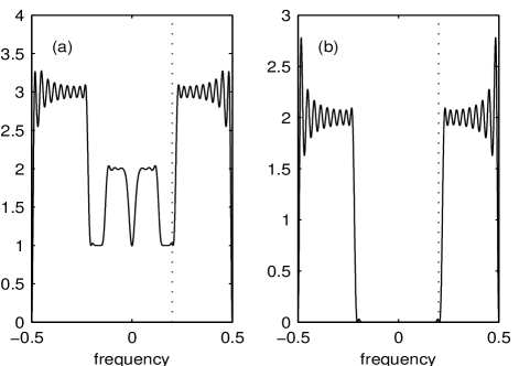
Figure 1: (a) $S_{Z}(f)$ and (b) $R_{Z}(f).$ The vertical dotted line marks the frequency $f=0.2.$

For $p\geq 2$ we will show that using the scaled $F$ approximation test where we reject $H_{0}$ if (51) holds brings about a worthwhile accuracy improvement over Box’s approximation test where we reject $H_{0}$ if

$$M(f)>\frac{K}{K-p}\chi_{2p^{2}}^{2}(1-\alpha).$$ (52)

To be able to do this we need to simulate from a model such that ${{\boldsymbol{S}}}_{{\boldsymbol{U}}}(f)$ in (6) has ${\boldsymbol{R}}_{{\boldsymbol{Z}}}(f)={\bf 0}$ for some frequency range. We can proceed as follows.

We know [25] that any complex second-order stationary scalar process (assumed zero mean here), whether proper or improper, can be written as the output of a widely linear filter driven by proper white noise, i.e.,

$$Z_{t}=\sum_{l=-\infty}^{\infty}g_{l}\epsilon_{t-l}+\sum_{l=-\infty}^{\infty}h_{l}\epsilon_{t-l}^{*},$$ (53)

where $\{g_{l}\}$ and $\{h_{l}\}$ are sequence of complex constants, and $\{\epsilon_{t}\}$ is proper white noise for which $\mbox{cov}\{\epsilon_{t+\tau},\epsilon_{t}\}=\sigma_{\epsilon}^{2}\delta_{\tau,0}\quad\mbox{and}\quad\mbox{cov}\{\epsilon_{t+\tau},\epsilon_{t}^{*}\}=0,$ for $\tau\in{\mathbb{Z}},$ where $\delta_{j,k}$ is the Kronecker delta. For simulation purposes it is convenient to set $\sigma_{\epsilon}^{2}=1.$ Then [25]

$$S_{Z}(f) = |G(f)|^{2}+|H(f)|^{2}$$ (54)

$$R_{Z}(f) = G(f)H(-f)+G(-f)H(f),$$ (55)

where $G(f)$ is the frequency response function of $\{g_{l}\}$ given by $G(f)=\sum_{l=-\infty}^{\infty}g_{l}{\rm e}^{-{\rm i}2\pi fl}$ and $H(f)$ is the frequency response function of $\{h_{l}\}.$

For $p\geq 2$ we generate processes $\{Z_{j,t}\},j=1,\ldots,p,$ such that

$$Z_{j,t} =\sum_{l=-\infty}^{\infty}g_{l}\epsilon_{j,t-l}+\sum_{l=-\infty}^{\infty}h_{l}\epsilon_{j,t-l}^{*}$$ (57)

$$\qquad+\sum_{l=-\infty}^{\infty}a_{l}{\bar{\epsilon}}_{j,t-l}+\sum_{l=-\infty}^{\infty}a_{l}{\bar{\epsilon}}_{j,t-l}^{*},$$

where the $2p$ processes $\{\{\epsilon_{j,t}\},\{{\bar{\epsilon}}_{j,t}\},j=1,\ldots,p\}$ are all independent of each other. The filter $\{g_{l}\}$ was chosen to be low-pass with a frequency transition zone $[0.125,0.15].$ The filter $\{h_{l}\}$ was of ‘Hilbert-type’ or all-pass in the frequency zone $[0.05,0.45].$ Thus $G(f)$ is real and symmetric while $H(f)$ is imaginary and skew-symmetric. According to (55), if using just these two filters, the resulting $R_{Z}(f)$ is zero for $f\in[-0.5,0.5].$ However, the filter $\{a_{l}\}$ was chosen to be high-pass above $f=0.2$ and therefore generates non-zero $R_{Z}(f)$ values at these high frequencies. The resulting $S_{Z}(f)$ and $R_{Z}(f)$ are shown in Fig. 1.

The matrix ${\boldsymbol{S}}_{{\boldsymbol{Z}}}(f)$ is thus of the form ${\boldsymbol{S}}_{{\boldsymbol{Z}}}(f)=S_{{\boldsymbol{Z}}}(f){\boldsymbol{I}}_{p}$ with frequency dependence as shown in Fig. 1(a) while ${\boldsymbol{R}}_{{\boldsymbol{Z}}}(f)$ is of the form ${\boldsymbol{R}}_{{\boldsymbol{Z}}}(f)=R_{{\boldsymbol{Z}}}(f){\boldsymbol{I}}_{p}$ with frequency dependence as shown in Fig. 1(b). We can thus simulate from this model to evaluate our hypothesis tests, knowing that for frequencies where ${\boldsymbol{R}}_{{\boldsymbol{Z}}}(f)={\bf 0}$ in fact ${\boldsymbol{S}}_{{\boldsymbol{Z}}}(f)\not={\bf 0}$ and thus (31) is well-defined.

$$\begin{array}[]{|c||c|ccccc|}\hline\cr&&&&f&&\\ (p,K)&100\alpha\%&0.06&0.12&0.18&0.24&0.42\\ \hline\cr\hline\cr(2,6)&1\%&1.5&1.5&1.4\quad\vline&31.1&35.4\\ &&1.1&1.1&0.9\quad\vline&25.8&30.0\\ \cline{2-7}\cr&5\%&6.1&6.2&6.3\quad\vline&60.0&63.6\\ &&5.0&5.1&5.2\quad\vline&55.3&59.3\\ \hline\cr\hline\cr(3,8)&1\%&2.0&2.1&2.2\quad\vline&55.7&58.9\\ &&{0.9}&{1.1}&{1.1}\quad\vline&{42.3}&{45.5}\\ \cline{2-7}\cr&5\%&8.2&8.3&8.3\quad\vline&81.0&82.9\\ &&{4.9}&{5.1}&{5.2}\quad\vline&{72.6}&{75.2}\\ \hline\cr\end{array}$$

TABLE II: Rejection percentages over 10 000 repetitions. The top line of each entry is for Box’s $\chi^{2}$ approximation (43) and the lower line is for the $F$ approximation of (51).

Sample results are shown in Table II for $(p,K)=(2,6)$ and $(3,8).$ So here $K=6$ and 8 are indeed small. Here $N=512$ but smaller time series lengths such as 128 produced very similar results. Shown are rejection percentages for $H_{0}$ over $10\,000$ independent repetitions. The nominal rates are shown in the second column. The first three columns of rejection percentages are for frequencies where ${\boldsymbol{R}}_{{\boldsymbol{Z}}}(f)={\bf 0},$ ($H_{0}$ is true) and the latter two are for frequencies where ${\boldsymbol{R}}_{{\boldsymbol{Z}}}(f)\not={\bf 0}$ ($H_{0}$ is false) — see Fig. 1(b). The top line of each entry is for Box’s $\chi^{2}$ approximation (52) and the lower line is for the $F$ approximation of (51). We see that, proportionately, the latter has a much more accurate rejection rate than Box’s approximation when $H_{0}$ is true, but is slightly less accurate when $H_{0}$ is false.

IX Data Analysis

Here we apply our results to ocean current speed and direction time series recorded at a mooring in the Labrador Sea [4, 17, 18]. We associate the eastward (zonal) measurement of current speed with $\{X_{t}\}$ and the northward (meridional) measurement with $\{Y_{t}\}$ and thus obtain the complex-valued series from (2). Series were recorded at six depths, (110, 760, 1260, 1760, 2510 and 3476m). The series are labelled 1 to 6 with increasing depth. We used $N=1600$ observations for the $6$-vector-valued complex time series, with a sampling interval of $\Delta_{\rm t}=1$hr. In the spectral analysis $K=12$ sine tapers were applied. Since $W_{N}$ in (15) is $0.004$c/hr, the validity range $W_{N}\leq|f|\leq f_{\cal N}-W_{N}$ for our statistical results for a finite-$N$ sample is given by $0.004\leq|f|\leq 0.496$c/hr. There was no evidence to reject the Gaussian assumption for this data set [5].

Of great interest to oceanographers are deep ocean motions well away from boundaries, especially in the internal wave frequency band. We pay special attention to low frequencies $f\in[0.02,0.14],$ in the internal wave band and near to the semi-diurnal tidal frequency. The so-called ‘inertial frequency’ is approximately $0.07$c/hr for this latitude and purely clockwise rotation occurs at the inertial frequency in the Northern hemisphere, making a band centred around the inertial frequency particularly interesting to study for such complex-valued processes. The dominant semi-diurnal tide at around $f=0.08$c/hr was estimated and removed to avoid spectral leakage affecting estimation near the inertial frequency.

For this data ${\boldsymbol{Z}}_{t}=[Z_{1,t},\ldots,Z_{6,t}]^{T}.$ In order to use different depth-contiguous sets of series we shall use the shorthand ${\boldsymbol{Z}}_{m:m^{\prime}}{\,{\displaystyle{\mathrel{\mathop{=}^{\rm def}}}}\,}[Z_{m,t},\ldots,Z_{m^{\prime},t}]^{T}$ with $1\leq m<m^{\prime}\leq 6.$

IX-A Concentration of Canonical Coherencies

The degree of polarization of a single random vector measures the spread amongst the eigenvalues of its covariance matrix. A random vector is completely polarized/unpolarized if all of its energy is concentrated in one direction/equally distributed amongst all dimensions. This idea can be extended to the correlation between two random vectors by defining the correlation spread [27] which provides a single, normalized measure of how much of the overall correlation is concentrated in a few coefficients, i.e., correlation is contained in a low dimensional subspace.

Using the analogous definition to [27] in our context we have coherence spread defined by

$$\sigma^{2}_{p}(f){\,{\displaystyle{\mathrel{\mathop{=}^{\rm def}}}}\,}\frac{p}{p-1}\left(\frac{\sum_{i=1}^{p}l^{4}_{j}(f)}{(\sum_{i=1}^{p}l^{2}_{j}(f))^{2}}-\frac{1}{p}\right).$$ (58)

If only one canonical coherence is non-zero, then $\sigma_{p}^{2}(f)=1,$ whereas if all canonical coherences are equal, $\sigma^{2}_{p}(f)=0.$ We note that if for a given $f$, $\sigma^{2}_{p}(f)=1$, the likelihood ratio test statistic $T(f)=\prod_{j=1}^{p}(1-l^{2}_{j}(f))=0,$ i.e. achieves its minimum value, implying ${{\boldsymbol{R}}}_{{\boldsymbol{Z}}}(f)\not={\bf 0}.$ Of course, for $\sigma_{p}^{2}(f)<1$ we are not able to conclude anything. In practice, we can only obtain an estimate $\hat{\sigma}_{p}^{2}(f)$ — where the $l_{j}^{2}(f)$ are replaced by the $\ell_{j}^{2}(f)$ — and therefore, the hypothesis test must be used to check for ${{\boldsymbol{R}}}_{{\boldsymbol{Z}}}(f)={\bf 0}.$

Fig. 2 displays $\hat{\sigma}_{p}^{2}(f)$ for vector time series (a) ${\boldsymbol{Z}}_{1:2}$, (b) ${\boldsymbol{Z}}_{1:3}$, (c) ${\boldsymbol{Z}}_{1:4}$, (d)${\boldsymbol{Z}}_{1:5}$ and (e) ${\boldsymbol{Z}}_{1:6}$. An immediate observation is that the coherence spread estimate for ${\boldsymbol{Z}}_{1:2}$ is highly erratic, with many values close to one. This is in contrast to all other plots where the spread ranges from $0.15-0.8$ gradually decreasing in range as we consider time series at increasing depths. A notable feature of (b) ${\boldsymbol{Z}}_{1:3}$ is the broader peaks around $0.05,0.065$ and $0.11$ and we see how the spread changes as we go from (b) ${\boldsymbol{Z}}_{1:3}$ to (c) ${\boldsymbol{Z}}_{1:4}$ with the broader peaks at $0.05$ and $0.11$ remaining intact whereas the one at $0.065$ shrinks from its value of $0.7$ to $0.4$; the sharper peaks at $0.08,0.09$ and $0.138$ disappear and a new peak appears at $0.044$ which persists in both (d) ${\boldsymbol{Z}}_{1:5}$ and (e) ${\boldsymbol{Z}}_{1:6}$. We have thus seen how an additional series (depth) notably changes the concentration level of the overall coherence at some frequencies while disturbing it much less at others.

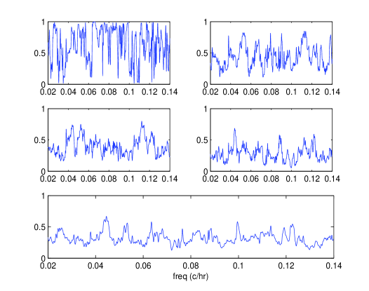
Figure 2: Coherence spread estimate $\hat{\sigma}_{p}^{2}(f)$ for time series vectors (left to right, top to bottom): (a) ${\boldsymbol{Z}}_{1:2}$, (b) ${\boldsymbol{Z}}_{1:3}$, (c) ${\boldsymbol{Z}}_{1:4},$ (d) ${\boldsymbol{Z}}_{1:5}$ and (e) ${\boldsymbol{Z}}_{1:6}$.

IX-B Test for Propriety

As defined in Section II-B the process $\{{\boldsymbol{Z}}_{t}\}$ is proper when ${{\boldsymbol{R}}}_{{\boldsymbol{Z}}}(f)={\bf 0}\,\,\text{for all}\,\,|f|\leq f_{\cal N}.$ Our test for $H_{0}:{\boldsymbol{R}}_{{\boldsymbol{Z}}}(f)={\mathbf{0}}$ is valid, and may be carried out, for any $W_{N}<f<f_{\cal N}-W_{N}.$

We test the same sets of time series for propriety and the results are displayed in Fig. 3. The solid line shows the test statistic $M(f)$ and the dotted line shows the critical value for each case. The test rejects $H_{0}$ at frequencies where $M(f)$ exceeds the critical value (thick line portions). The dashed line is the semi-diurnal tidal frequency. The coherence spread for ${\boldsymbol{Z}}_{1:2}$ (first subplot in Fig. 2) takes the maximum value of $0.9927$ at $f=0.065,$ very close to the inertial frequency, and Fig. 3 (a) shows that our test rejects $H_{0}$ around this frequency very clearly. The band of frequencies around $0.04$ is most prominent with rejection also clearly visible at frequencies $0.027,0.075$ and $0.087$. For ${\boldsymbol{Z}}_{1:3}$, the test rejects $H_{0}$ for almost the same set of low frequencies with rejection also at a higher frequency around $0.12$. Results for ${\boldsymbol{Z}}_{1:4}$ are very similar to that for ${\boldsymbol{Z}}_{1:3}$, the main difference being that a small frequency band near $0.1$ also rejects $H_{0}.$ In general, we see that as other series (deeper in the ocean) are considered, $H_{0}$ is rejected, not only at low frequencies but also due to some additional higher frequencies, but less definitively so. Importantly then, Fig. 3 shows which frequency bands cause propriety to be rejected.

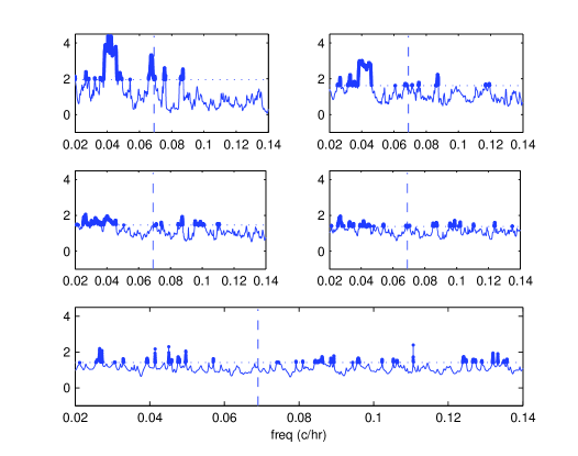
Figure 3: The test statistic $M(f)$ (solid) and the critical value (dotted line) for (left to right, top to bottom): (a) ${\boldsymbol{Z}}_{1:2}$, (b) ${\boldsymbol{Z}}_{1:3}$, (c) ${\boldsymbol{Z}}_{1:4},$ (d) ${\boldsymbol{Z}}_{1:5}$ and (e) ${\boldsymbol{Z}}_{1:6}$. The test rejects the null hypothesis of propriety at frequencies where $M(f)$ exceeds the critical value (thick line portions). The dashed line is the semi-diurnal tidal frequency.

X Other Measures of Vector Coherence

From Lemma 1, one measure for vector coherence is the sum of all the canonical coherencies:

$${\rm tr}\{{\boldsymbol{S}}_{{\boldsymbol{Z}}}^{-1}(f){\boldsymbol{R}}_{{\boldsymbol{Z}}}(f){\boldsymbol{S}}^{-T}_{{\boldsymbol{Z}}}(-f){\boldsymbol{R}}_{{\boldsymbol{Z}}}^{H}(f)\}=\sum_{j=1}^{p}l_{j}^{2}(f).$$ (59)

Levikov and Sokolov [16] looked for a coefficient of coherence in the case of two real-valued vector random processes. In our paper, for the vector ${\boldsymbol{V}}_{t}=[{\boldsymbol{X}}_{t}^{T},{\boldsymbol{Y}}^{T}_{t}]^{T},$ we consider $\{{\boldsymbol{X}}_{t}\}$ and $\{{\boldsymbol{Y}}_{t}\}$ to be two geometrically related vector components and combine them to form a complex-valued vector time series. Levikov and Sokolov did not consider the two processes to be related in such a way and treated them simply as two vector process. They did, however, make use of the frequency domain and derived the quantity

$$\beta^{2}(f)\mathrel{\mathop{=}^{\rm def}}\frac{1}{2}[{\boldsymbol{P}}(f){\boldsymbol{S}}_{{\boldsymbol{Y}}{\boldsymbol{Y}}}^{-1}(f)+{\boldsymbol{S}}_{{\boldsymbol{Y}}{\boldsymbol{Y}}}^{-1}(f){\boldsymbol{P}}(f)],$$

where ${\boldsymbol{P}}(f)={\boldsymbol{S}}_{{\boldsymbol{Y}}{\boldsymbol{X}}}(f){\boldsymbol{S}}_{{\boldsymbol{X}}{\boldsymbol{X}}}^{-1}(f){\boldsymbol{S}}_{{\boldsymbol{Y}}{\boldsymbol{X}}}^{H}(f).$ Taking the trace of this quantity we get

$$\!\!\!\!\!\!\!{\rm tr}\{\beta^{2}(f)\}\!\!\!\! = \!\!\!\!\frac{1}{2}{\rm tr}\{{\boldsymbol{P}}(f){\boldsymbol{S}}_{{\boldsymbol{Y}}{\boldsymbol{Y}}}^{-1}(f)+{\boldsymbol{S}}_{{\boldsymbol{Y}}{\boldsymbol{Y}}}^{-1}(f){\boldsymbol{P}}(f)\}$$ (60)

$$= \!\!\!\!{\rm tr}\{{\boldsymbol{P}}(f){\boldsymbol{S}}_{{\boldsymbol{Y}}{\boldsymbol{Y}}}^{-1}(f)\}$$

$$= \!\!\!\!{\rm tr}\{{\boldsymbol{S}}_{{\boldsymbol{Y}}{\boldsymbol{X}}}(f){\boldsymbol{S}}_{{\boldsymbol{X}}{\boldsymbol{X}}}^{-1}(f){\boldsymbol{S}}_{{\boldsymbol{Y}}{\boldsymbol{X}}}^{H}(f){\boldsymbol{S}}_{{\boldsymbol{Y}}{\boldsymbol{Y}}}^{-1}(f)\}$$

$$= \!\!\!\!{\rm tr}\{{\boldsymbol{S}}_{{\boldsymbol{X}}{\boldsymbol{X}}}^{-1}(f){\boldsymbol{S}}_{{\boldsymbol{X}}{\boldsymbol{Y}}}(f){\boldsymbol{S}}_{{\boldsymbol{Y}}{\boldsymbol{Y}}}^{-1}(f){\boldsymbol{S}}_{{\boldsymbol{Y}}{\boldsymbol{X}}}(f)\}.$$

This is of the same form as (59) only now using the components of the partition in (5); it will be the sum of all the canonical coherencies between ${\rm d}{\boldsymbol{Z}}_{\boldsymbol{X}}(f)$ and ${\rm d}{\boldsymbol{Z}}_{\boldsymbol{Y}}(f)$ where

$${\boldsymbol{X}}_{t}=\int_{-f_{\cal N}}^{f_{\cal N}}{\rm e}^{{\rm i}2\pi ft}\,{\rm d}{\boldsymbol{Z}}_{\boldsymbol{X}}(f);\,\,{\boldsymbol{Y}}_{t}=\int_{-f_{\cal N}}^{f_{\cal N}}{\rm e}^{{\rm i}2\pi ft}\,{\rm d}{\boldsymbol{Z}}_{\boldsymbol{Y}}(f).$$

Now ${\boldsymbol{Z}}_{t}={\boldsymbol{X}}_{t}+{\rm i}{\boldsymbol{Y}}_{t}$ and ${\boldsymbol{Z}}^{*}_{t}={\boldsymbol{X}}_{t}-{\rm i}{\boldsymbol{Y}}_{t}.$ The spectral representation gives ${\rm d}{\boldsymbol{Z}}(f)={\rm d}{\boldsymbol{Z}}_{\boldsymbol{X}}(f)+{\rm i}\,{\rm d}{\boldsymbol{Z}}_{\boldsymbol{Y}}(f)$ and ${\rm d}{\boldsymbol{Z}}^{*}(-f)={\rm d}{\boldsymbol{Z}}_{\boldsymbol{X}}(f)-{\rm i}\,{\rm d}{\boldsymbol{Z}}_{\boldsymbol{Y}}(f).$ So we can write

$$\left[\begin{matrix}{\rm d}{\boldsymbol{Z}}(f)\\ {\rm d}{\boldsymbol{Z}}^{*}(-f)\end{matrix}\right]={{\boldsymbol{T}}}\left[\begin{matrix}{\rm d}{\boldsymbol{Z}}_{\boldsymbol{X}}(f)\\ {\rm d}{\boldsymbol{Z}}_{\boldsymbol{Y}}(f)\end{matrix}\right],$$ (61)

where ${\boldsymbol{T}}$ is given in (3). We know that affine transformations of ${\rm d}{\boldsymbol{Z}}_{\boldsymbol{X}}(f)$ and of ${\rm d}{\boldsymbol{Z}}_{\boldsymbol{Y}}(f)$ will not change the canonical coherencies; however, (61) does not represent affine transforms of ${\rm d}{\boldsymbol{Z}}_{\boldsymbol{X}}(f)$ and of ${\rm d}{\boldsymbol{Z}}_{\boldsymbol{Y}}(f)$ since a mixing is involved.

Hence the quantities (59) and (60) will in general be different. Indeed for the example of Section VIII the value of (60) is zero over $|f|\leq 1/2,$ because ${\boldsymbol{S}}_{{\boldsymbol{X}}{\boldsymbol{Y}}}(f)={\boldsymbol{S}}_{{\boldsymbol{Y}}{\boldsymbol{X}}}(f)={\bf 0}.$

XI Summary and Conclusion

We have developed a frequency domain approach to test for propriety of complex-valued vector time series. For propriety of $\{{\boldsymbol{Z}}_{t}\}$ we require ${{\boldsymbol{R}}}_{{\boldsymbol{Z}}}(f)={\bf 0}\,\,\text{for all}\,\,|f|\leq f_{\cal N}.$ We can carry out the test $H_{0}:{\boldsymbol{R}}_{{\boldsymbol{Z}}}(f)={\mathbf{0}}$ for any $W_{N}<f<f_{\cal N}-W_{N}.$ Most importantly for the vector case $(p\geq 2)$ we have justified use of the rule that $H_{0}$ is rejected if $M(f)=-2K\log T(f)>bF_{\nu_{1},\nu_{2}}(1-\alpha).$ There is no assumption that $K$ is large, and indeed this would rarely be expected in practice. We have shown in detail how the statistic $T(f)$ arises by consideration of canonical coherencies for complex-valued vector time series. When propriety is invalid, the frequency domain approach has the scientific advantage of showing which frequency bands are causing rejection, likely allowing linkage to known or hypothesized properties of the physical processes involved.

-A Proof of Lemma 1

Given (21), since ${\boldsymbol{S}}_{{\boldsymbol{Z}}}(f)$ and ${\boldsymbol{S}}^{T}_{{\boldsymbol{Z}}}(-f)$ are positive-definite (Hermitian) covariance matrices, we have solutions

$${\boldsymbol{A}}^{H}(f) = {\boldsymbol{F}}^{H}(f){\boldsymbol{S}}_{{\boldsymbol{Z}}}^{-1/2}(f)$$ (62)

$${\boldsymbol{B}}^{H}(f) = {\boldsymbol{G}}^{H}(f){\boldsymbol{S}}^{-T/2}_{{\boldsymbol{Z}}}(-f)$$ (63)

where ${\boldsymbol{F}}(f),{\boldsymbol{G}}(f)\in{\mathbb{C}}^{p\times p}$ are unitary. Then

$$\!\!\!\!\!\!\!\!\!\!\!\!{\boldsymbol{K}}(f) = {\boldsymbol{A}}^{H}(f){\boldsymbol{R}}_{{\boldsymbol{Z}}}(f){\boldsymbol{B}}(f)$$ (64)

$$= {\boldsymbol{F}}^{H}(f){\boldsymbol{S}}_{{\boldsymbol{Z}}}^{-1/2}(f){\boldsymbol{R}}_{{\boldsymbol{Z}}}(f){\boldsymbol{S}}^{-T/2}_{{\boldsymbol{Z}}}(-f){\boldsymbol{G}}(f).$$

We now make use of the weak majorization result [28, p. 294]. Let $|{\rm diag}({\boldsymbol{K}}(f))|\,{\displaystyle{\mathrel{\mathop{=}^{\rm def}}}}\,[|K_{11}(f)|,\ldots,|K_{pp}(f)|]^{T}.$ Then

$$\sum_{j=1}^{r}|K_{[jj]}(f)|\leq\sum_{j=1}^{r}|\sigma_{[j]}(f)|,\,r=1,\ldots,p.$$

where the $\sigma_{j}(f)$ are the singular values of ${\boldsymbol{K}}(f)$ and $\sigma_{[1]}(f)\geq\sigma_{[2]}(f)\geq\cdots\geq\sigma_{[p]}(f),$ (a descending size order). Hence the solution to (23) is found by making ${\boldsymbol{K}}(f)$ diagonal. From (64), we thus choose ${\boldsymbol{F}}(f)$ and ${\boldsymbol{G}}(f)$ to diagonalize ${\boldsymbol{K}}(f),$ i.e., ${\boldsymbol{F}}(f)$ and ${\boldsymbol{G}}(f)$ are determined by singular value decomposition of

$${\boldsymbol{C}}(f)\mathrel{\mathop{=}^{\rm def}}{\boldsymbol{S}}_{{\boldsymbol{Z}}}^{-1/2}(f){\boldsymbol{R}}_{{\boldsymbol{Z}}}(f){\boldsymbol{S}}^{-T/2}_{{\boldsymbol{Z}}}(-f)={\boldsymbol{F}}(f){\boldsymbol{K}}(f){\boldsymbol{G}}^{H}(f),$$

giving

$${\boldsymbol{C}}(f){\boldsymbol{C}}^{H}(f)\!\!\!\! = \!\!\!\!{\boldsymbol{S}}_{{\boldsymbol{Z}}}^{-1/2}(f){\boldsymbol{R}}_{{\boldsymbol{Z}}}(f){\boldsymbol{S}}^{-T}_{{\boldsymbol{Z}}}(-f){\boldsymbol{R}}^{H}_{{\boldsymbol{Z}}}(f){\boldsymbol{S}}_{{\boldsymbol{Z}}}^{-1/2}(f)$$

$$= \!\!\!\!{\boldsymbol{F}}(f){\boldsymbol{L}}(f){\boldsymbol{F}}^{H}(f),$$

where ${\boldsymbol{L}}(f)$ denotes a diagonal matrix with $j$th element $l_{j}^{2}(f)=|K_{jj}(f)|^{2},$ in descending size order. Now multiply through on the left by ${\boldsymbol{S}}_{{\boldsymbol{Z}}}^{-1/2}(f)$ and on the right by ${\boldsymbol{F}}(f)$ to obtain

$$\!\!\!\!\!\!\!\!\!\!\!\!\!\!\!\!\!\!\!\!\!\!\!\!\!\!\!\!\!\!\!\!{\boldsymbol{S}}_{{\boldsymbol{Z}}}^{-1}(f){\boldsymbol{R}}_{{\boldsymbol{Z}}}(f){\boldsymbol{S}}^{-T}_{{\boldsymbol{Z}}}(-f){\boldsymbol{R}}^{H}_{{\boldsymbol{Z}}}(f){\boldsymbol{S}}_{{\boldsymbol{Z}}}^{-1/2}(f){\boldsymbol{F}}(f)$$

$$= \!\!\!\!{\boldsymbol{S}}_{{\boldsymbol{Z}}}^{-1/2}(f){\boldsymbol{F}}(f){\boldsymbol{L}}(f),$$

which, using (62), can be written

$${\boldsymbol{S}}_{{\boldsymbol{Z}}}^{-1}(f){\boldsymbol{R}}_{{\boldsymbol{Z}}}(f){\boldsymbol{S}}^{-T}_{{\boldsymbol{Z}}}(-f){\boldsymbol{R}}^{H}_{{\boldsymbol{Z}}}(f){\boldsymbol{A}}(f)={\boldsymbol{A}}(f){\boldsymbol{L}}(f),$$

so that

$${\boldsymbol{S}}_{{\boldsymbol{Z}}}^{-1}(f){\boldsymbol{R}}_{{\boldsymbol{Z}}}(f){\boldsymbol{S}}^{-T}_{{\boldsymbol{Z}}}(-f){\boldsymbol{R}}^{H}_{{\boldsymbol{Z}}}(f){\boldsymbol{A}}_{j}(f)=l_{j}^{2}(f){\boldsymbol{A}}_{j}(f),$$

and $l_{j}^{2}(f)$ are the eigenvalues, and ${\boldsymbol{A}}_{j}(f)$ are the eigenvectors of the $p\times p$ matrix ${\boldsymbol{S}}_{{\boldsymbol{Z}}}^{-1}(f){\boldsymbol{R}}_{{\boldsymbol{Z}}}(f){\boldsymbol{S}}^{-T}_{{\boldsymbol{Z}}}(-f){\boldsymbol{R}}^{H}_{{\boldsymbol{Z}}}(f),$ as required. Note that this matrix is the product of the two Hermitian matrices ${\boldsymbol{S}}_{{\boldsymbol{Z}}}^{-1}(f)$ and ${\boldsymbol{R}}_{{\boldsymbol{Z}}}(f){\boldsymbol{S}}^{-T}_{{\boldsymbol{Z}}}(-f){\boldsymbol{R}}^{H}_{{\boldsymbol{Z}}}(f).$

Similarly,

$${\boldsymbol{C}}^{H}(f){\boldsymbol{C}}(f)\!\!\!\! = \!\!\!\!{\boldsymbol{S}}^{-T/2}_{{\boldsymbol{Z}}}(-f){\boldsymbol{R}}^{H}_{{\boldsymbol{Z}}}(f){\boldsymbol{S}}_{{\boldsymbol{Z}}}^{-1}(f){\boldsymbol{R}}_{{\boldsymbol{Z}}}(f){\boldsymbol{S}}^{-T/2}_{{\boldsymbol{Z}}}(-f)$$

$$= \!\!\!\!{\boldsymbol{G}}(f){\boldsymbol{L}}(f){\boldsymbol{G}}^{H}(f).$$

Multiply through on the left by ${\boldsymbol{S}}_{{\boldsymbol{Z}}}^{-T/2}(f)$ and on the right by ${\boldsymbol{G}}(f),$ and use (63) to obtain

$${\boldsymbol{S}}_{{\boldsymbol{Z}}}^{-T}(-f){\boldsymbol{R}}_{{\boldsymbol{Z}}}^{H}(f){\boldsymbol{S}}^{-1}_{{\boldsymbol{Z}}}(f){\boldsymbol{R}}_{{\boldsymbol{Z}}}(f){\boldsymbol{B}}(f)={\boldsymbol{B}}(f){\boldsymbol{L}}(f),$$

so that, as required

$${\boldsymbol{S}}^{-T}_{{\boldsymbol{Z}}}(-f){\boldsymbol{R}}_{{\boldsymbol{Z}}}^{H}(f){\boldsymbol{S}}_{{\boldsymbol{Z}}}^{-1}(f){\boldsymbol{R}}_{{\boldsymbol{Z}}}(f){\boldsymbol{B}}_{j}(f)=l_{j}^{2}(f){\boldsymbol{B}}_{j}(f).$$

$l_{j}^{2}(f)$ are the eigenvalues, and ${\boldsymbol{B}}_{j}(f)$ are the eigenvectors of the $p\times p$ matrix ${\boldsymbol{S}}^{-T}_{{\boldsymbol{Z}}}(-f){\boldsymbol{R}}_{{\boldsymbol{Z}}}^{H}(f){\boldsymbol{S}}_{{\boldsymbol{Z}}}^{-1}(f){\boldsymbol{R}}_{{\boldsymbol{Z}}}(f).$

Notice that the matrices ${\boldsymbol{S}}_{{\boldsymbol{Z}}}^{-1}(f){\boldsymbol{R}}_{{\boldsymbol{Z}}}(f){\boldsymbol{S}}^{-T}_{{\boldsymbol{Z}}}(-f){\boldsymbol{R}}^{H}_{{\boldsymbol{Z}}}(f)$ and ${\boldsymbol{S}}^{-T}_{{\boldsymbol{Z}}}(-f){\boldsymbol{R}}_{{\boldsymbol{Z}}}^{H}(f){\boldsymbol{S}}_{{\boldsymbol{Z}}}^{-1}(f){\boldsymbol{R}}_{{\boldsymbol{Z}}}(f)$ are just cyclic permutations of each other.

Finally,

$${\rm cov}\{{\rm d}{\boldsymbol{Z}}_{{\boldsymbol{\xi}}}(f),{\rm d}{\boldsymbol{Z}}_{{\boldsymbol{\eta}}}(f)\}=E\{{\rm d}{\boldsymbol{Z}}_{{\boldsymbol{\xi}}}(f){\rm d}{\boldsymbol{Z}}^{H}_{{\boldsymbol{\eta}}}(f)\}={\boldsymbol{K}}(f),$$

and the solution of the optimization problem makes ${\boldsymbol{K}}(f)$ diagonal. Hence, ${\rm corr}\{{\rm d}Z_{\xi_{j}}(f),{\rm d}Z_{\eta_{k}}(f)\}=0,\,\,\,\mbox{for}\,\,\,j,k=1,\ldots,p;j\not=k.$

-B Proof of Lemma 2

To simplify notation we drop explicit frequency dependence. Consider the distribution of $T=l_{G}^{1/K},$ given by (38), under the null hypothesis. We have

$$E\{T^{r}\}=\int\cdots\int{\textstyle{\frac{[\det\{{\boldsymbol{A}}\}]^{r}}{[\det\{{\boldsymbol{A}}_{11}\}\det\{{\boldsymbol{A}}_{22}\}]^{r}}}}g({{\boldsymbol{A}}}){\rm d}{\boldsymbol{A}},$$

where $g({\boldsymbol{A}})$ is the PDF for the complex Wishart distribution. As explained in the text under the null hypothesis we can take ${\boldsymbol{S}}_{{\boldsymbol{U}}}$ to be ${\boldsymbol{I}}_{2p}$ because of invariance under the group action. We can thus replace (36) by

$${\boldsymbol{A}}\mathrel{\mathop{=}^{\rm d}}{\cal W}^{C}_{2p}(K,{\boldsymbol{I}}_{2p}),$$

and using [11] we know that for ${\boldsymbol{A}}>0,K\geq 2p,$

$$g({\boldsymbol{A}};K,2p,{\boldsymbol{I}}_{2p})=c(K,2p)[\det\{{\boldsymbol{A}}\}]^{K-2p}{\rm e}^{-{\rm tr}\{{\boldsymbol{A}}\}},$$ (65)

where $c(K,2p)$ is a constant defined by

$$c^{-1}(K,2p)=\pi^{p(2p-1)}\prod_{i=1}^{2p}\Gamma(K+1-i).$$ (66)

So $E\{T^{r}\}$ takes the form

$$\!\!\!\!\!\!\!\!\!\!\!\!\!\!\!\!c(K,2p)\int\cdots\int{\textstyle{\frac{[\det\{{\boldsymbol{A}}\}]^{K-2p+r}}{[\det\{{\boldsymbol{A}}_{11}\}\det\{{\boldsymbol{A}}_{22}\}]^{r}}}}{\rm e}^{-{\rm tr}\{{\boldsymbol{A}}\}}{\rm d}{\boldsymbol{A}}$$

$$\!\!\!\!\!\!\!\!\!\!\!\!\!\!\!\!={{\frac{c(K,2p)}{c(K+r,2p)}}}\int\cdots\int{\textstyle{\frac{1}{[\det\{{\boldsymbol{A}}_{11}\}\det\{{\boldsymbol{A}}_{22}\}]^{r}}}}$$

$$\times\left[c(K+r,2p)[\det\{{\boldsymbol{A}}\}]^{K-2p+r}{\rm e}^{-{\rm tr}\{{\boldsymbol{A}}\}}\right]{\rm d}{\boldsymbol{A}}.$$

The integration is w.r.t. ${\rm d}{\boldsymbol{A}}={\rm d}A_{11},\ldots,{\rm d}A_{2p2p}.$ The term in the square brackets above is the PDF for the ${\cal W}^{C}_{2p}(K+r,{\boldsymbol{I}}_{2p})$ distribution. The integral of this density with respect to the elements in ${\boldsymbol{A}}_{12}$ and ${\boldsymbol{A}}_{21}$ must give the marginal density of ${\boldsymbol{A}}_{11},{\boldsymbol{A}}_{22},$ which is the product

$$g({\boldsymbol{A}}_{11};K+r,p,{\boldsymbol{I}}_{p})\cdot g({\boldsymbol{A}}_{22};K+r,p,{\boldsymbol{I}}_{p}),$$ (67)

since ${\boldsymbol{A}}_{11}$ and ${\boldsymbol{A}}_{22}$ are independent under the null hypothesis. Carrying out the integration and using (65) and (67) we obtain

$$\!\!\!\!\!\!\!\!\!\!\!\!\!\!\!{{\frac{c(K,2p)}{c(K+r,2p)}}}\int\cdots\int{\textstyle{\frac{1}{[\det\{{\boldsymbol{A}}_{11}\}\det\{{\boldsymbol{A}}_{22}\}]^{r}}}}$$

$$\!\!\!\!\!\!\!\!\!\!\!\times\prod_{j=1}^{2}c(K+r,p)[\det\{{\boldsymbol{A}}_{jj}\}]^{K+r-p}{{\rm e}}^{-{\rm tr}\{{\boldsymbol{A}}_{jj}\}}{{\rm d}}{{\boldsymbol{A}}}_{jj}$$

$$\!\!\!\!\!\!\!\!\!\!\!\!={{\frac{c(K,2p)}{c(K+r,2p)}}}\prod_{j=1}^{2}\int\cdots\int c(K+r,p)[\det\{{\boldsymbol{A}}_{jj}\}]^{K-p}$$

$$\times\quad{{\rm e}}^{-{\rm tr}\{{\boldsymbol{A}}_{jj}\}}{{\rm d}}{{\boldsymbol{A}}}_{jj}$$

$$={{\frac{c(K,2p)}{c(K+r,2p)}}}\prod_{j=1}^{2}\frac{c(K+r,p)}{c(K,p)}.$$ (68)

Using (66) and (68) we get

$$\!E\{T^{r}\}\!=\!\frac{\prod_{j=1}^{2p}\Gamma(K\!+\!r+1-j)[\prod_{j=1}^{p}\Gamma(K\!+\!1-j)]^{2}}{\prod_{j=1}^{2p}\Gamma(K\!+\!1-j)[\prod_{j=1}^{p}\Gamma(K\!+\!r+1-j)]^{2}}.$$ (69)

This agrees with [14, eqn. (2.6)] which appears without reference or proof. Now $T^{r}=l_{G}^{r/K}$ so if we let $r\rightarrow rK,$ then $T^{rK}=l_{G}^{r}.$ So

$$\!\!\!\!\!\!\!\!\!\!\!E\{l_{G}^{r}\}\!=\!\frac{\prod_{j=1}^{2p}\Gamma(K[1+r]+1-j)\prod_{j=1}^{p}\Gamma(K\!+\!1\!-\!j)}{\prod_{j=1}^{2p}\Gamma(K\!+\!1\!-\!j)\prod_{j=1}^{p}\Gamma(K[1+r]+1-j)}$$

$$\times\left[\frac{\prod_{j=1}^{p}\Gamma(K\!+\!1\!-\!j)}{\prod_{j=1}^{p}\Gamma(K[1+r]+1-j)}\right]$$

$$=\frac{\prod_{j=1}^{p}\Gamma(K[1+r]+1-j-p)}{\prod_{j=1}^{p}\Gamma(K+1-j-p)}$$

$$\times\left[\frac{\prod_{j=1}^{p}\Gamma(K\!+\!1\!-\!j)}{\prod_{j=1}^{p}\Gamma(K[1+r]+1-j)}\right]$$

$$=\left[\frac{\prod_{j=1}^{p}\Gamma(K\!+\!1\!-\!j)}{\prod_{j=1}^{p}\Gamma(K+1-j-p)}\right]$$

$$\times\frac{\prod_{j=1}^{p}\Gamma(K[1+r]+1-j-p)}{\prod_{j=1}^{p}\Gamma(K[1+r]+1-j)},$$

which is (39).

-C Proof of Lemma 3

Under the null hypothesis the $r$th moment of $T(f)$ is

$$E\{T^{r}(f)\}=\prod_{j=1}^{p}\frac{\Gamma(K+r+1-j-p)\Gamma(K+1-j)}{\Gamma(K+r+1-j)\Gamma(K+1-j-p)}.$$ (70)

To see this start with (69) and proceeed in analogous vein to the last part of the proof of Lemma 2; since we are continuing to look at $E\{T^{r}\}$ the step $r\rightarrow rK$ is not made. Note that when $j=p$ the critical gamma function argument is still positive: $K+r+1-j-p=K+r+1-2p>0$ since $K\geq 2p$ with $r\geq 0.$

A real scalar random variable $X$ is said to have a (type-1) beta distribution, $X\,\,{\displaystyle\mathrel{\mathop{=}^{\rm d}}}\,\,{\rm beta}(\alpha,\beta),$ if the PDF is

$$f(x)=\frac{\Gamma(\alpha+\beta)}{\Gamma(\alpha)\Gamma(\beta)}x^{\alpha-1}(1-x)^{\beta-1},\,\,0<x<1,\alpha>0,\beta>0.$$

The $r$th moment for this distribution is

$$E\{X^{r}\}=\frac{\Gamma(\alpha+r)\Gamma(\alpha+\beta)}{\Gamma(\alpha+\beta+r)\Gamma(\alpha)},\,\,\alpha+r>0.$$ (71)

Comparing (70) and (71) we see for a fixed $j$ that $\alpha=K+1-j-p$ and $\beta=p$ which gives the required result.

References

- [1] T. Adalı, P. J. Schreier & L. L. Scharf, “Complex-valued signal processing: the proper way to deal with impropriety,” IEEE Transactions on Signal Processing, vol. 59, pp. 5101–5125, 2011.
- [2] G. E. P. Box, “A general distribution theory for a class of likelihood criteria,” Biometrika, vol. 36, 317–46, 1949.
- [3] E. M. Carter, C. G. Khatri & M. S. Srivastava, “Nonnull distribution of likelihood ratio criterion for reality of covariance matrix,” J. Multivariate Analysis, vol. 6, pp. 176–184, 1976.
- [4] S. Chandna and A. T. Walden, “Statistical properties of the estimator of the rotary coefficient,” IEEE Transactions on Signal Processing, vol. 59, pp. 1298–1303, 2011.
- [5] S. Chandna and A. T. Walden, “Simulation methodology for inference on physical parameters of complex vector-valued signals,” IEEE Transactions on Signal Processing, vol. 61, pp. 5260–5269, 2013.
- [6] T. Chonavel, Statistical Signal Processing. London UK: Springer-Verlag, 2002.
- [7] S. Elipot and R. Lumpkin, “Spectral description of oceanic near-surface variability,” Geophys. Res. Lett. 35, L05606, 2008.
- [8] W. J. Emery and R. E. Thomson, Data Analysis Methods in Physical Oceanography. New York: Pergamon, 1998.
- [9] C. Fang, P. R. Krishnaiah and B. N. Nagarsenker, “Asymptotic distributions of the likelihood ratio test statistics for covariance structures of the complex multivariate normal distributions,” J. Multivariate Analysis, vol. 12, pp. 597–611, 1982.
- [10] P. Ginzberg, “Quaternion matrices: statistical properties and applications to signal processing and wavelets,” Ph. D. dissertation, Dept. Mathematics, Imperial College London, 2013.
- [11] N. R. Goodman, “Statistical analysis based on a certain multivariate complex Gaussian distribution (an introduction),” Ann. Math. Statist., vol. 34, pp. 152–77, 1963.
- [12] A. K. Gupta, “Distribution of Wilks’ likelihood-ratio criterion in the complex case,” Ann. Instit. Statist. Math., vol. 23, pp. 77–87, 1971.
- [13] A. K. Gupta, “On a test for reality of the covariance matrix in a complex Gaussian distribution,” J. Statist. Computation and Simulation, vol. 2, pp. 333-342, 1973.
- [14] P. R. Krishnaiah,, J. C. Lee and T. C. Chang, “The distributions of the likelihood ratio statistics for tests of certain covariance structures of complex multivariate normal populations,” Biometrika, vol. 63, pp. 543–549, 1976.
- [15] P. R. Krishnaiah,, J. C. Lee and T. C. Chang, “Likelihood ratio tests on covariance matrices and mean vectors of complex multivariate normal populations and their applications in time series,” Technical report TR-83-03, Center for Multivariate Analysis, Univ. Pittsburgh, 1983.
- [16] S. Levikov and S. Sokolov, “Coefficient of coherence in the case of two vector random processes,” Deep-Sea Research Part I: Oceanographic Research Papers, vol. 44, pp. 1329–1338, 1997.
- [17] J. M. Lilly, P. B. Rhines, M. Visbeck, R. Davis, J. R. Lazier, F. Schott and D. Farmer, “Observing deep convection in the Labrador Sea during winter 1994/95,” J. Phys. Oceanogr., vol. 29, 2065–98, 1999.
- [18] J. M. Lilly and P. B. Rhines, “Coherent eddies in the Labrador Sea observed from a mooring,” J. Phys. Oceanogr., vol. 32, 585–98, 2002.
- [19] C. N. K. Mooers, “A technique for the cross spectrum analysis of pairs of complex-valued time series, with emphasis on properties of polarized components and rotational invariants,” Deep-Sea Research, vol. 20, pp. 1129–1141, 1973.
- [20] W. Min and R. S. Tsay, “On canonical analysis of multivariate time series,” Statistica Sinica, vol. 15, pp. 303–323, 2005.
- [21] M. Miyata, “Complex generalization of canonical correlation and its application to a sea-level study,” J. Marine Research, vol. 28, pp. 202–214, 1970.
- [22] J. Navarro-Moreno, M. D. Estudillo-Martínez, R. M. Fernández-Alcalá & J. C. Ruiz-Molina, “Estimation of improper complex-valued random signals in colored noise by using the Hilbert space theory,” IEEE Trans. Inf. Theory, vol. 55, pp. 2859–2867, 2009.
- [23] E. Ollila and V. Koivunen, “Generalized complex elliptical distributions,” in Proc. Third Sensor Array and Multichannel Signal Processing Workshop, Sitges, Spain, July, 2004, pp. 460–4.
- [24] B. Picinbono, “Second-order complex random vectors and normal distributions,” IEEE Transactions on Signal Processing vol. 44, pp. 2637–2640, 1996.
- [25] B. Picinbono and P. Bondon, “Second-order statistics of complex signals,” IEEE Trans. Signal Processing, vol. 45, pp. 411–420, 1997.
- [26] G. Reinsel, Elements of Multivariate Time Series Analysis (2nd Ed). New York: Springer, 1997.
- [27] P. J. Schreier, “A unifying discussion of correlation analysis for complex random vectors,” IEEE Transactions on Signal Processing, vol. 56, pp. 1327–1336, 2008.
- [28] P. J. Schreier and L. L. Scharf, Statistical Signal Processing of Complex-Valued Data, Cambridge UK: Cambridge University Press, 2010.
- [29] P. J. Schreier, L. L. Scharf and A. Hanssen, “A generalized likelihood ratio test for impropriety of complex signals,” IEEE Signal Process. Lett., vol. 13, pp. 433–6, 2006.
- [30] A. M. Sykulski, S. C. Olhede, J. M. Lilly & J. J. Early, “On parametric modelling and inference for complex-valued time series,” ArXiv preprint arXiv:1306.5993v2, 2015. Available:http://arxiv.org/abs/1306.5993.
- [31] A. M. Sykulski, S. C. Olhede & J. M. Lilly, “An improper complex autoregressive process of order one,” ArXiv preprint arXiv:1511.04128v1, 2015. Available:http://arxiv.org/abs/1511.04128.
- [32] H. van Haren and C. Millot, “Rectilinear and circular inertial motions in the Western Mediterranean Sea,” Deep-Sea Research Part I, vol. 51, pp. 1441–55, 2004.
- [33] A. T. Walden, “Rotary components, random ellipses and polarization: a statistical perspective,” Phil. Trans. R. Soc. A, vol. 371, doi:10.1098/rsta.2011.0554, 2013.
- [34] A. T. Walden and P. Rubin-Delanchy, “On testing for impropriety of complex-valued Gaussian vectors,” IEEE Transactions on Signal Processing vol. 57, pp. 825–834, 2009.
- [35] A. T. Walden, E. J. McCoy and D. B. Percival, “The effective bandwidth of a multitaper spectral estimator,” Biometrika, vol. 82, 201–214, 1995.
- [36] A. M. Yaglom, Correlation Theory of Stationary and Related Random Functions, Volume I: Basic Results. New York: Springer, 1987.
- [37] G. A. Young and R. L.Smith, Essentials of Statistical Inference. Cambridge UK: Cambridge University Press, 2005.