Wirelessly Powered Backscatter Communication Networks: Modeling, Coverage and Capacity

Abstract

Future Internet-of-Things (IoT) will connect billions of small computing devices embedded in the environment and support their device-to-device (D2D) communication. Powering these massive number of embedded devices is a key challenge of designing IoT since batteries increase the devices’ form factors and battery recharging/replacement is difficult. To tackle this challenge, we propose a novel network architecture that enables D2D communication between passive nodes by integrating wireless power transfer and backscatter communication, which is called a wirelessly powered backscatter communication (WP-BackCom) network. In this network, standalone power beacons (PBs) are deployed for wirelessly powering nodes by beaming unmodulated carrier signals to targeted nodes. Provisioned with a backscatter antenna, a node transmits data to an intended receiver by modulating and reflecting a fraction of a carrier signal. Such transmission by backscatter consumes orders-of-magnitude less power than a traditional radio. Thereby, the dense deployment of low-complexity PBs with high transmission power can power a large-scale IoT. In this paper, a WP-BackCom network is modeled as a random Poisson cluster process in the horizontal plane where PBs are Poisson distributed and active ad-hoc pairs of backscatter communication nodes with fixed separation distances form random clusters centered at PBs. The backscatter nodes can harvest energy from and backscatter carrier signals transmitted by PBs. Furthermore, the transmission power of each node depends on the distance from the associated PB. Applying stochastic geometry, the network coverage probability and transmission capacity are derived and optimized as functions of backscatter parameters, including backscatter duty cycle, reflection coefficient, and the PB density. The effects of the parameters on network performance are characterized.

I Introduction

Internet-of-Things (IoT) is envisioned as a future network to connect billions of small computing devices embedded in the environment (e.g., walls and furniture) and implanted in bodies and enable their device-to-device (D2D) wireless communication. Powering a massive number of such devices remains a key design challenge for IoT. Batteries add to devices’ weights and form factors and battery recharging/replacement increases the maintenance cost if not infeasible. To handle this challenge, we propose a novel network architecture that enables large-scale passive IoT deployment by seamlessly integration of wireless power transfer (WPT) [1, 2] and low-power backscattering communication [3], called a wirelessly powered backscatter communication (WP-BackCom) network. Specifically, power beacons (PBs) that are stations dedicated for WPT [4] are deployed for wirelessly powering dense backscatter D2D links and each node transmits data by reflecting and modulating the carrier signals sent by PBs. This work aims at modeling and analyzing the performance of a WP-BackCom network. To be specific, the network is modeled as Poisson cluster processes and its coverage and capacity are analyzed using stochastic geometry.

I-A Backscatter Communication

Backscatter communication refers to a design where a radio device transmits data via reflecting and modulating an incident radio frequency (RF) signal by adapting the level of antenna impedance mismatch to vary the reflection coefficient and furthermore harvests energy from the signal for operating the circuit [5, 3]. Backscatter devices do not require oscillators to generate carrier signals that are obtained from the air instead. Furthermore, using the simple analog modulation scheme, the device requires no analog-to-digital converters (ADCs) used in the case of digital modulation. As a result of these features, a backscatter transmitter consumes power orders-of-magnitude less than a conventional radio. Traditionally, backscatter communication is widely used in the application of radio-frequency Identification (RFID) where a reader powers and communicates with a RFID tag over a short range no more than typically of several meters [6, 7]. Recent years have seen the development of more sophisticated backscatter communication systems and advancement in the underpinning communication theory [8, 9, 10, 11, 12]. To reduce tag complexity, estimation of forward (for WPT) and backward (for information transfer) channels is usually performed at the reader that transmits and receives a training signal over different antennas. The close-loop propagation makes it difficult to estimate the two channels separately, which are required for transmit and receive beamforming. A channel-estimation algorithm for energy beamforming is proposed in [8] that alleviates this difficulty by exploiting the structure of a backscatter channel to improve WPT efficiency. Multiple-access in a backscatter network is studied in [9]. By treating collision of backscatter nodes as a sparse code, a novel approach is proposed in [9] that resolves the collisions using sparse sensing algorithm and rateless-code decoding algorithm. The work in [10] addresses the issue of security in backscatter communication by proposing the technique of injecting a noise-like signal into the carrier signal sent by a reader to avoid eavesdropping of the backscatter signal. In [11], a variation of the backscatter communication system with an improved range is proposed, which has the key feature of detaching the carrier transmitter from the reader and placing it near the tag. Based on the new system design, the bit-error-rate performance of various modulation schemes is analyzed. Last, a new system based on ultra-wide bandwidth (UWB) is developed in [12]. The advantage of such a system is that based on time-hopping spread spectrum, the huge processing gain arising from signaling using ultra-sharp pulses eliminates interference between coexisting backscatter communication links.

The traditional reader-tag configuration is unsuitable for IoT since typical nodes are energy-constrained and may not be able to wirelessly power other nodes for communications over sufficiently long distances. This motivated the design of a backscatter communication system powered by RF energy harvesting, where the transmission of a backscatter node relies on harvesting energy and reflecting incident RF signals from the ambient environment such as TV, Wi-Fi and cellular signals [13, 14, 15]. From the perspective of energy-source systems (e.g., TV, Wi-Fi or cellular systems), the effect of coexisting backscatter transmitters is to generate addition multi-paths. The systems have two drawbacks. First, to avoid mutual interference between coexisting systems, backscatter links have much lower data rates (using the on/off-keying modulation) than the energy-source links. Second, backscatter communication networks based on ambient RF energy harvesting do not have scalability due to their dependance on other networks as energy sources. Thus, they may not be suitable for implementing large-scale dense IoT with relatively high rates. This motivates the design of WP-BackCom network architecture where WPT can deliver power much higher than that by energy harvesting and low-complexity backhaul-less PBs are widely deployed to power dense passive D2D links.

I-B Modeling the WP-BackCom Network

To study the performance of a large-scale WP-BackCom network, we adopt stochastic geometry to design and analyze wireless networks (a survey can be found in e.g., [16]). Among various types of spatial point processes, Poisson cluster process (PCP), where daughter points form random clusters centered at points from a parent Poisson point process (PPP), are commonly used for modeling wireless networks with random cluster topologies arising from geographical factors or protocols for medium access control [17, 18]. In particular, in recent work on random networks, PCPs have been frequently used to model the phenomenons of user clustering at hotspots [19] and the clustering of small-cell base stations (BSs) around macro-cell BSs [20] for heterogeneous networks or distributed-node clustering in D2D networks [21]. In this work, the WP-BackCom network is also modeled as a PCP where PBs form the parent PPP and backscatter nodes are the clustered daughter points. The clustering phenomenon arises from the fact that only nodes lying within a given distance from the nearest PB can harvest sufficient energy for operating their circuits and powering their transmissions. In other words, active backscatter nodes are effectively attracted to PBs, thereby forming clusters with PBs at their centers. The location of a node can be uniformly distributed in a circle or normally scattered with a given variance around the centered affiliated PB, yielding the Matern and Thomas cluster processes, respectively. The use of dedicated stations similar to PBs instead of relaying on readers for powering backscatter nodes is also observed in [11] to improve the link bit-error-rate performance. Relying on WPT from PBs, nodes’ transmission power depends on their distances from the associated PBs. In contrast, in the conventional network models, transmission power of BSs/nodes is independent of their locations. The location-dependent transmission power in the WP-BackCom network as well as other practical factors (e.g., circuit power consumption, backscatter duty cycle, reflection coefficient, etc.) introduce new challenges for network performance analysis.

Recently, stochastic geometry has been also applied to model large-scale energy harvesting (including WPT) networks building on existing network architectures including cellular networks [4, 22], relay networks [23, 24], heterogeneous networks [25], cognitive networks [26], and general networks with mutually repulsive nodes [27]. In particular, the WP-BackCom network is similar to cellular networks with WPT considered in [4, 22] where PBs are deployed to power passive nodes’ transmissions. Nevertheless, the current work faces new theoretical challenges arising from a new network topology based on a PCP instead of PPPs in the prior work. Furthermore, practical factors arising from backscatter also introduce a new dimension for network performance optimization.

I-C Summary of Contributions and Organization

The mentioned model of random network topology corresponds to a normal WP-BackCom network with the nodes density exceeding that of PBs. Consider the models of backscatter transmission and channels. Time is divided into slots, each of which is further divided into mini-slots. For an arbitrary slot, each transmitting node performs backscatter transmission as well as energy harvesting in a randomly selected mini-slot and only energy harvesting in other mini-slots. The fraction of time used for transmission is referred to as the duty cycle. Furthermore, for transmission, the fraction of backscattered incident energy is called the reflection coefficient. The condition required for backscatter transmission is that the total energy harvested by a transmitting node within each slot exceeds the energy consumed by the circuit, introducing a circuit-power constraint. Next, a PB beams a carrier signal with fixed power to each target node over a free-space channel with only path loss. Moreover, the pairs of communicating nodes have unit distances and their channels have both fading and path loss.

To the best of our knowledge, this paper presents the first attempt to model and analyze a large-scale backscatter communication network using stochastic geometry. The theoretic contributions of this paper are summarized as follows.

1. The interference distribution is analyzed. Given the PCP, the interference power for a typical receiver is decomposed into intra-cluster and inter-cluster interference. Their characteristic functionals are derived for the normal WP-BackCom network and their product gives that for the total interference power.

2. The distribution of node-transmission power is also investigated. A key variable characterizing the transmission power of a transmitting node is the probability, called the power-outage probability, that the circuit-power constraint is not satisfied, corresponding to insufficient energy for turning on the node. The probability is derived in closed-form.

3. Consider the network coverage measured by the metric of success probability defined as the probability that the transmission over a typical D2D link is successful. The results in 1) and 2) are applied to derive a lower bound on the success probability. The result reveals that the success probability is a convex function of the reflection coefficient and can be thus maximized over this parameter.

4. Consider the network transmission capacity defined as the density of reliable and active backscatter D2D links. In the regime of almost-full network coverage (with close-to-one success probability), the capacity is shown to be a convex function of the duty cycle and a monotone decreasing function of the reflection coefficient for most of range. Based on the result, the network capacity is optimized.

5. In addition, we also consider a network with dense PBs. The corresponding model is modified from the counterpart for the normal network by denoting the parent points as transmitting nodes and the daughter points as PBs. Then the results for the normal network are extended to the network with dense PBs.

The reminder of this paper is organized as follows. The mathematical models and performance metrics are described in Section II. Section III presents the interference characteristic functionals and transmission power distribution for WP-BackCom networks. The network coverage and capacity are analyzed in Section IV and V, respectively. Simulation results are presented in Section VI followed by concluding remarks in Section VII.

Notation: Given $X\in\mathds{R}^{2}$, $|X|$ denotes the Euclidean distance from $X$ to the origin. For a set $\mathcal{X}$, $|\mathcal{X}|$ yields its cardinality. The set-subtraction operator is denoted as $\backslash$.

Table I: Summary of Notation

Notation	Meaning
$\Pi_{\text{pb}}$, $\lambda_{\text{pb}}$	The PPP modeling PBs in a normal WP-BackCom network, its density
$\tilde{\Phi}_{\text{nd}}$, $\lambda_{\text{pb}}\bar{c}$	The PCP modeling transmitting nodes in the normal WP-BackCom network, its density
$\Phi_{\text{nd}}$, $\lambda_{\text{pb}}\bar{c}D$	The PCP modeling backscatter nodes in the normal WP-BackCom network, its density
$\Pi_{\text{nd}}$, $\lambda_{\text{nd}}D$	The PPP modeling backscatter nodes in the WP-BackCom network with dense PBs, its density
$\Phi_{\text{pb}}$, $\lambda_{\text{nd}}\bar{m}$	The PCP modeling PBs in the WP-BackCom network with dense PBs, its density
$Y_{0},X_{0},Z_{0}$	Typical PB, transmitting node, intended receiver
$\eta$, $g$	Transmission power, beamforming gain for each PB
$P_{X}$	Received power at a backscatter node $X$
$\alpha_{1}$, $\alpha_{2}$	Path-loss exponents for the WPT links, the D2D backscatter links
$h$	Rayleigh fading coefficient
$D$, $\beta$	Duty cycle, backscatter reflection coefficient
$P_{c}$	Circuit power consumption
$\theta$	SIR threshold for success D2D backscatter transmission
$P_{s}$, $p_{0}$, $C$	Success probability of backscatter communication, power-outage probability, network transmission capacity

II Mathematical Models and Metrics

The mathematical models and performance metrics are discussed in the following sub-sections. The notation used this work is summarized in Table I.

II-A Spatial Network Models

II-A1 Normal WP-BackCom Network

Consider the normal WP-BackCom network where the PB density is smaller than that of backscatter nodes. This normal PBs model is constructed using a PCP as follows. Let $\Pi_{\text{pb}}=\{Y_{0},Y_{1},\cdots\}$ denote a PPP in the horizontal plane with density $\lambda_{\text{pb}}$ modeling the locations of PBs. Consider a cluster of mobile transmitting nodes centered at the origin, denoted as $\widetilde{\mathcal{N}}=\{X_{0},X_{1},\cdots,X_{N}\}$. The number of nodes, $N$, is a Poisson random variable (r.v.) with mean $\bar{c}$. The r.v., $X_{n}\in\mathds{R}^{2}$, represents the location of the corresponding node and $\{X_{n}\}$ are independent and identically distributed (i.i.d.). For an arbitrary r.v. $X_{n}$, the direction is isotropic and the distance to the origin, $|X_{n}|$, has one of two possible probability density functions (PDFs), resulting in the Matern and Thomas cluster processes. Let the function $f:\mathds{R}^{+}\rightarrow\mathds{R}^{+}$ denote the PDF of the distance from a cluster member’s location to the cluster center, denoted as $r$, which is defined as follows:

$$\text{(Matern c.p.)}\quad f(r) =\begin{cases}\frac{1}{\pi a^{2}},&0\leq r\leq a,\\ 0,&\mbox{otherwise,}\end{cases}$$ (1)

$$\text{(Thomas c.p.)}\quad f(r) =\frac{1}{2\pi\sigma^{2}}\exp\left(-\frac{r^{2}}{2\sigma^{2}}\right),$$ (2)

where $a$ and $\sigma^{2}$ are positive constants representing the cluster radius and the variance, respectively. Let $\{\widetilde{\mathcal{N}}_{Y}\}$ denote a sequence of clusters constructed by generating an i.i.d. sequence of clusters having the same distribution as $\widetilde{\mathcal{N}}$ and translating them to be centered at the points $\{Y\}\in\Pi_{\text{pb}}$. Then the process of transmitting nodes, denoted as $\tilde{\Phi}_{\text{nd}}$, can be written as $\tilde{\Phi}_{\text{nd}}=\bigcup_{Y\in\Pi_{\text{pb}}}\widetilde{\mathcal{N}}_{Y}$. The density of $\tilde{\Phi}_{\text{nd}}$ is $\lambda_{\text{pb}}\bar{c}$. The link from a PB to an intended transmitting node is called a WPT link. Each transmitting node is paired with an intended receiving node that is located at a unit distance and in an isotropic direction, forming a D2D backscatter transmission link. Fig. 1 shows two network realizations generated based on the Matern and Thomas cluster processes, which helps to visualize the topology of Poisson clustered network as well as the WPT links.

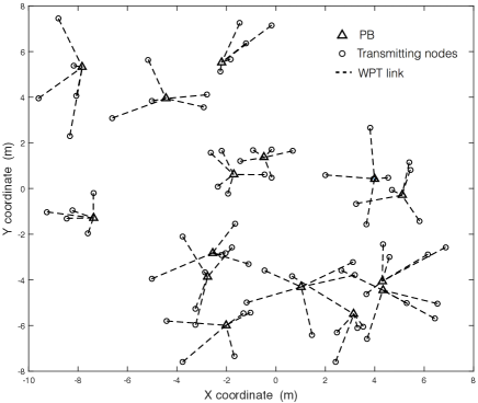
(a) Normal PBs model: Matern cluster process

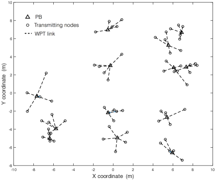
(b) Normal PBs model: Thomas cluster process

Figure 1: The spatial distribution of the normal WP-BackCom network modeled using the (a) Matern cluster process and (b) Thomas cluster process.

Time is divided into slots with unit duration. Each slot is further divided into $M$ mini-slots. A transmitting node randomly selects a single mini-slot to transmit signal by backscattering and the selection remains unchanged over slots. The selections by different nodes are assumed independent. This divides each slot into a backscatter phase and a waiting phase of durations $1/M$ and $(1-1/M)$, respectively. The duty cycle, denoted as $D$, is given as $D=1/M$. A transmitting node in a backscatter phase is called a backscatter node. Then the backscatter-node process, denoted as $\Phi$, and a cluster of backscatter nodes centered at $Y$, denoted as $\mathcal{N}_{Y}$, can be obtained from $\tilde{\Phi}_{\text{nd}}$ and $\widetilde{\mathcal{N}}_{Y}$ by independent thinning. As a result, $\Phi_{\text{nd}}$ has the density of $\lambda_{\text{pb}}\bar{c}D$ and the expected number of nodes in $\mathcal{N}_{Y}$ is $\bar{c}D$.

II-A2 WP-BackCom Network with Dense PBs

Consider the case where the PB density exceeds that of backscatter nodes. The corresponding network model with dense PBs is modified from the normal network model by switching the locations of the PBs and transmitting nodes. Specifically, the model comprises a PCP where the parent PPP, denoted as $\Pi_{\text{nd}}$, models the random locations of backscatter nodes and the PBs are the daughter points, denoted as $\Phi_{\text{pb}}$. The density of $\Pi_{\text{nd}}$ is $\lambda_{\text{nd}}D$ with $\lambda_{\text{nd}}$ representing the density of transmitting nodes. By abusing the notation, let $\bar{m}$ represent the expected number of PBs in each cluster of $\Phi_{\text{pb}}$ and $\mathcal{N}_{X}$ represent a cluster of PBs centered at the backscatter node $X$. It follows that $\Phi_{\text{pb}}=\bigcup_{X\in\Pi_{\text{nd}}}\mathcal{N}_{X}$. Fig. 2 shows the dense PBs case of Thomas cluster process.

Figure 2: The WP-BackCom network with dense PBs: Thomas cluster process.

II-B Channel Model

II-B1 Channel Model for the Normal WP-BackCom Network

PBs are equipped with antenna arrays and nodes have single isotropic antennas. Each PB beams the continuous wave (CW) to nodes in its corresponding cluster. A PB serves multiple backscatter nodes simultaneously where the total transmission power is adapted to the number of nodes to guarantee the quality-of-service. Specifically, a PB beams transmission power of $\eta$ to each intended node and thus the expected total transmission power is equal to $\eta$ times the number of nodes in the corresponding cluster (the expectation is $\bar{c}\eta$). Given beamforming and relatively short distance for efficient WPT, each WPT link is suitably modeled as a channel with path loss but no fading [1, 4]. As a result, with a typical PB at $Y_{0}$, the receive power at a typical node $X_{0}$ is given as $P_{X_{0}}=\eta g|X_{0}-Y_{0}|^{-\alpha_{1}}$ where $g>0$ denotes the beamforming gain and $\alpha_{1}$ represents the path loss exponent for WPT links. Due to beamforming, it is assumed that each node harvests negligible energy from other PBs and data signals compared with that from the serving PB. When transmitting, a node backscatters a fraction, called a reflection coefficient and denoted as $\beta\in[0,1]$, of $P_{X}$ such that the signal power received at the typical receiver at $Z_{0}$ is $\beta P_{X_{0}}h_{X_{0}}$ where $h_{X_{0}}\sim\exp(1)$ models Rayleigh fading. A transmitting node may not be able to transmit if there is insufficient energy for operating its circuit as discussed in the sequel. This constraint is represented by a function $\ell(\cdot)$, which is defined in the sequel (the following sub-section), such that the transmission power of the backscatter node $X$ can be written as $\beta\ell(P_{X})$. The interference power measured at $Z_{0}$ can be written as

$$I=\sum_{X\in\Phi_{\text{nd}}\backslash\{X_{0}\}}\beta\ell(P_{X})h_{X}|X-Z_{0}|^{-\alpha_{2}},$$ (3)

where $\{h_{X}\}$ are i.i.d. $\exp(1)$ r.v.s modeling Rayleigh fading, $\alpha_{2}$ represents the path loss exponent for interference (D2D) links. Recall that $\tilde{\Phi}_{\text{nd}}$ and $\Phi_{\text{nd}}$ with $\Phi_{\text{nd}}\subseteq\tilde{\Phi}_{\text{nd}}$ represent (both active and inactive) transmitting nodes and (active) backscatter nodes provisioned with sufficient energy, respectively. Thus, the interference power in (3) is a sum over $\Phi_{\text{nd}}$ instead of $\tilde{\Phi}_{\text{nd}}$. It is worth mentioning that the signal transmitted from PB is unmodulated carrier that appears as a DC level after down-conversion, which can be easily removed and thus not considered as interference as those modulated ones.

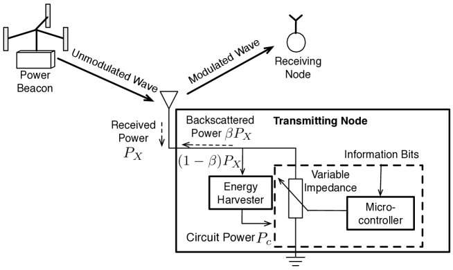
Figure 3: Wirelessly powered backscatter communication.

II-B2 Channel Model for the Network with Dense PBs

The total power received at the typical node $X_{0}$ is contributed by beamforming PBs in the corresponding cluster. As a result, $P_{X_{0}}$ can be written as $P_{X_{0}}=\eta g\sum_{Y\in\mathcal{N}_{X_{0}}}|X_{0}-Y|^{-\alpha_{1}}$. Moreover, the power of interference as measured at the typical receiver $Z_{0}$ is given as

$$I=\sum_{X\in\Pi_{\text{nd}}\backslash\{X_{0}\}}\beta\ell(P_{X})h_{X}|X-Z_{0}|^{-\alpha_{2}}.$$ (4)

II-C Backscatter Communication Model

The operation of WP-BackCom network is illustrated in Fig. 3. Consider the backscatter phase of an arbitrary slot. A transmitting node adapts the variable impedance (or equivalently its level of mismatch with the antenna impedance) shown in the figure so as to modulate the backscattered CW with information bits [3]. Given a transmitting node at $X$ and the reflection coefficient $\beta$, the backscattered power is $\beta P_{X}$ with the remainder $(1-\beta)P_{X}$ consumed by the circuit or harvested [28]. Next, for the waiting phase, the transmitting node withholds transmission and performs only energy harvesting. It is assumed that the circuit of each transmitting node consumes fixed power denoted as $P_{c}$. To be able to transmit, a node has to harvest sufficient energy for powering the circuit, resulting in the following circuit-power constraint: $(1-\beta)P_{X}D+P_{X}(1-D)\geq P_{c}$. This gives

$$\text{(Circuit-power constraint)}\quad P_{X}\geq\frac{P_{c}}{1-\beta D}.$$ (5)

Consequently, a node transmits or is silent depending on if the constraint is satisfied. Under the circuit-power constraint given in (5), a transmission power of the typical transmitting node can be written as $\beta\ell(P_{X_{0}})$ where the function $\ell(P)$ gives $P$ if $P\geq P_{c}/(1-\beta D)$ or else is equal to $0$. This function is also used in the interference power in (3) and (4).

II-D Performance Metrics

The network performance is measured by two metrics, namely the success probability and the network transmission capacity. The success probability is denoted as $P_{s}$. Assuming an interference limited network, the condition for successful transmission is that the receive signal-to-interference ratio (SIR) exceeds a fixed positive threshold $\theta$. The assumption of negligible noise (or equivalently interference limited network) can be justified as follows. The installation of PBs for powering short-distance D2D links can result in relatively large signal power and increase the density of coexisting active D2D links that have strong mutual interference. As a rule of thumb, the network is interference limited if the expected interference power is much larger than the noise variance, resulting in conditions on network parameters. For instance, it is straightforward to derive a threshold on the PB density for the interference-limited regime.

Then the success probability is given as

$$P_{s}=\Pr\left(\beta\ell(P_{X_{0}})h_{X_{0}}\geq\theta I\right).$$ (6)

To facilitate the analysis, the total interference will be partitioned into two parts, intra-cluster and inter-cluster interference, for characterizing its distribution in the next section.

The other metric is network (transmission) capacity denoted as $C$ and defined as:

$$C=\left\{\begin{aligned} &B\lambda_{\text{pb}}\bar{c}DP_{s},&&\text{normal network},\\ &B\lambda_{\text{nd}}DP_{s},&&\text{network with dense PBs},\end{aligned}\right.$$ (7)

where the factor $B$ represents the data rate per D2D link and the other factor is the spatial density of active links with successful transmission [17, 29]. It follows that $C$ quantifies the network spatial throughput and has the unit of b/s/Hz/unit-area. Without loss of generality, $B$ is set as $1$ (b/s/Hz) to simplify notation.

III Interference and Transmission Power

In this section, for the WP-BackCom network, the distributions of interference at the typical receiver and the transmission power for the typical backscatter node are analyzed. The results are used subsequently for characterizing network coverage and capacity.

III-A Interference Characteristic Functionals

III-A1 Normal WP-BackCom Network

Let $\mathcal{C}(s)$ with $s>0$ denote the characteristic functional of the interference power $I$ given in (3): $\mathcal{C}(s)=\mathsf{E}\left[e^{-sI}\right]$. In this section, the characteristic functional of normal WP-BackCom network model is derived. Without loss of generality, consider a typical backscatter node at $X_{0}$ at the origin and the typical receiving node $Z_{0}=z$. To facilitate derivation, the total interference $I$ is split in the sequel into two components, the intra-cluster and inter-cluster interference, denoted as $I_{a}$ and $I_{b}$, respectively. The intra-cluster interference is caused by the interfering backscatter nodes inside the representative cluster (i.e., the cluster with typical backscatter node and receiver), and the inter-cluster interference is caused by simultaneously backscatter nodes outside the representative cluster. The separation of intra-cluster and inter-cluster is due to their difference in distribution. Specifically, the former depends on a cluster of random points with the typical one removed and the latter on a cluster point process with the typical cluster removed. They are defined and analyzed separately to yield insight into the structure of interference distribution.

Mathematically, $I=I_{a}+I_{b}$ where

$$I_{a} =\sum_{X\in\mathcal{N}_{0}\backslash\{X_{0}\}}\beta\ell(P_{X})h_{X}|X-z|^{-\alpha_{2}},$$ (8)

$$I_{b} =\sum_{Y\in\Pi_{\text{pb}}\backslash\{Y_{0}\}}\sum_{X\in\mathcal{N}_{Y}}\beta\ell(P_{X})h_{X}|X-z|^{-\alpha_{2}}.$$ (9)

Note that in $\eqref{Eq:InterInt}$, the first summation is over all other PBs not affiliated with the typical backscatter node (corresponding to clusters of interferers) and the second summation is over the cluster of interferers centered at the PB $Y$.

The characteristic functionals of $I_{a}$ and $I_{b}$ are denoted as $\mathcal{C}_{a}(s)$ and $\mathcal{C}_{b}(s)$, respectively, which are defined similarly as $\mathcal{C}(s)$. They are derived as shown in the following two lemmas.

Lemma 1 (Intra-cluster Interference in the Normal Network).

Given $s\geq 0$, the characteristic functional of the intra-cluster interference power $I_{a}$ is given as

$$\mathcal{C}_{a}(s)=\int_{\mathds{R}^{2}}\exp\Big{(}-\bar{c}Dq(s,y,z)\Big{)}f(|y|)dy,$$ (10)

where

$$q(s,y,z)=\int_{\mathds{O}}\frac{1}{1+(s\beta\eta g)^{-1}|x|^{\alpha_{1}}|x+y-z|^{\alpha_{2}}}f(|x|)dx,$$ (11)

$f(\cdot)$ is specified in (1) and (2), and the set $\mathds{O}$ arising from the circuit-power constraint is defined as

$$\mathds{O}=\left\{x\in\mathds{R}^{2}\mid|x|\leq\left(\frac{\eta g(1-\beta D)}{P_{c}}\right)^{\frac{1}{\alpha_{1}}}\right\}.$$ (12)

Proof: See Appendix -A.  $\Box$

Lemma 2 (Inter-cluster Interference in the Normal Network).

Given $s\geq 0$, the characteristic functional of the inter-cluster interference power $I_{b}$ is given as

$$\mathcal{C}_{b}(s)=\exp\Bigg{(}-\lambda_{\text{pb}}\int_{\mathds{R}^{2}}\Big{(}1-e^{-\bar{c}Dq(s,y,z)}\Big{)}dy\Bigg{)},$$ (13)

where $q(s,y,z)$ and the set $\mathds{O}$ are defined in Lemma 1.

Proof: See Appendix -B.  $\Box$

III-A2 Network with Dense PBs

In this model, the interferes are distributed as a homogeneous PPP instead of a PCP as in the normal network. Thus, it is unnecessary to decompose the total interference into intra- and inter-cluster interference. The total interference power can be written as

$$I^{{}^{\prime}} =\sum_{X\in\Pi_{\text{nd}}\backslash\{X_{0}\}}\beta\ell(P_{X})h_{X}|X-z|^{-\alpha_{2}}$$

$$=\sum_{X\in\Pi_{\text{nd}}\backslash\{X_{0}\}}\beta\ell\left(\sum_{Y\in\mathcal{N}_{X}}\eta g|Y-X|^{-\alpha_{1}}\right)h_{X}|X-z|^{-\alpha_{2}}.$$ (14)

It can be observed that the received power at each node is a sum over a cluster of PBs instead of a single PB in the normal network. For analytical tractability, relaxing the circuit-power constraint allows nodes that are previously inactive under this constraint to transmit, resulting in the following upper bound on the interference power:

$$I^{{}^{\prime}}\leq\beta\eta g\sum_{X\in\Pi_{\text{nd}}\backslash\{X_{0}\}}\left(\sum_{Y\in\mathcal{N}_{X}}|Y-X|^{-\alpha_{1}}\right)h_{X}|X-z|^{-\alpha_{2}}.$$ (15)

Notice that since each node is charged by multiple PBs, it is likely that the circuit-power constraints are satisfied at the majority of nodes and thus the lower bound in (15) is tight. Using this inequality, a lower bound on the characteristic functional of $I^{{}^{\prime}}$, denoted as $\mathcal{C}^{{}^{\prime}}(s)$, is obtained as shown in the following lemma.

Lemma 3 (Interference in the Network with Dense PBs).

Given $s\geq 0$, the characteristic functional of the interference power $I^{{}^{\prime}}$ satisfies

$$\mathcal{C}^{{}^{\prime}}(s)\geq\exp\Bigg{(}-\lambda_{\text{nd}}D\int_{\mathds{R}^{2}}\Big{(}1-e^{-\bar{m}u(s,x,z)}\Big{)}dx\Bigg{)},$$ (16)

where

$$u(s,x,z)=2\pi\int^{\infty}_{0}\frac{1}{1+(s\beta\eta g)^{-1}r^{\alpha_{1}}|x-z|^{\alpha_{2}}}f(r)rdr$$ (17)

and $f(\cdot)$ is specified in (1) and (2).

Proof: See Appendix -C.  $\Box$

Remark 1.

Comparing Lemma 2 and 3, the lower bounds on $\mathcal{C}_{b}(s)$ and $\mathcal{C}^{{}^{\prime}}(s)$ have similar expressions. The key difference is that the PB density ($\lambda_{\text{pb}}$) and expected number of backscatter nodes per cluster ($\bar{c}D$) in the former are replaced by the backscatter-node density ($\lambda_{\text{nd}}D$) and expected number of PBs per cluster ($\bar{m}$) in the latter. The similarity arises from that both network models are based on PCPs where the locations of backscatter nodes and PBs are swapped.

III-B Transmission-Power Distribution

III-B1 Normal WP-BackCom Network

Under the circuit-power constraint, there exists a threshold on the separation distance between a pair of PB and affiliated backscatter node:

$$d_{0}=\left[\frac{\eta g(1-\beta D)}{P_{c}}\right]^{\frac{1}{\alpha_{1}}},$$ (18)

such that the node’s transmission power is zero if the distance exceeds the threshold. Then transmission power (i.e., backscattered power) of the typical backscatter node, denoted as $P_{t}$, is given as $P_{t}=\beta\eta g|X_{0}-Y_{0}|^{-\alpha_{1}}$ if $|X_{0}-Y_{0}|\leq d_{0}$ or otherwise $P_{t}=0$. The event of $P_{t}=0$ corresponds that of circuit power outage. It follows that the power-outage probability, denoted as $p_{0}$, can be written as

$$p_{0}=\Pr(P_{t}=0)=2\pi\int_{d_{0}}^{\infty}f(r)rdr.$$ (19)

For the case where the circuit-power constraint is satisfied,

$$\Pr(P_{t}\geq\tau)=2\pi\int\limits_{0}^{(\beta\eta g/\tau)^{\frac{1}{\alpha_{1}}}}f(r)rdr,\ \ \tau\geq\frac{\beta P_{c}}{1-\beta D}.$$ (20)

Substituting the PDFs in (1) and (2) into (19) and (20) gives the following results.

Lemma 4 (Node Transmission Power for the Normal Network).

The transmission power of a typical backscatter node has support of $\{0\}\cup[\frac{\beta P_{c}}{1-\beta D},\infty]$. The power-outage probability, $p_{0}$, and the complementary cumulative distribution function (CCDF), denoted as $\bar{F}_{t}$, are given as follows.

• (Matern cluster process)

  $$p_{0} =\left\{\begin{aligned} &1-\left(\frac{d_{0}}{a}\right)^{2},&&d_{0}<a,\\ &0,&&\text{otherwise.}\end{aligned}\right.$$

  $$\bar{F}_{t}(\tau)=\Pr(P_{t}\geq\tau) =\left\{\begin{aligned} &\frac{1}{a^{2}}\left(\frac{\beta\eta g}{\tau}\right)^{\frac{2}{\alpha_{1}}},&&\tau>\frac{\beta\eta g}{a^{\alpha_{1}}}\\ &1,&&\text{otherwise,}\end{aligned}\right.$$

  with $\tau\in[\frac{\beta P_{c}}{1-\beta D},\infty]$.

• (Thomas cluster process)

  $$p_{0} =\exp\left(-\frac{d_{0}^{2}}{2\sigma^{2}}\right),$$

  $$\bar{F}_{t}(\tau) =1-\exp\left(-\frac{1}{2\sigma^{2}}\left(\frac{\beta\eta g}{\tau}\right)^{\frac{2}{\alpha_{1}}}\right),$$

  with $\tau\in[\frac{\beta P_{c}}{1-\beta D},\infty]$.

A sanity check is as follows. The distance threshold $d_{0}$ in (18) is a monotone decreasing function of both $\beta D$ and $P_{c}$. The reason is that increasing the duty cycle and reflection coefficient leads to less harvested energy thus adding the probability of circuit-power outage and improving the circuit power conumption has the same effect. Consequently, the power-outage probability decreases with increasing $d_{0}$ for both cases in Lemma 4. Next, the CCDFs in Lemma 4 are observed to be independent of $D$ but increase with growing $\beta$. The reason is that conditioned on the node transmitting, the transmission power depends only on the incident power from the PB scaled by $\beta$ but is independent of the duty cycle.

Remark 2 (Effects of $P_{c}$ on Power Outage).

Let $\{c_{n}\}$ denote a set of constants. For the Matern cluster process, the power-outage probability $p_{0}$ is a monotone increasing function of the circuit power $P_{c}$ and scales as $\left(1-c_{1}P_{c}^{-\frac{2}{\alpha_{1}}}\right)$. One can see that increasing the path loss exponent $\alpha_{1}$ alleviates the negative effect of increasing $P_{c}$ on power outage. In contrast, the scaling law for the Thomas cluster process is $\exp\left(-c_{2}P_{c}^{-\frac{2}{\alpha_{1}}}\right)$. Comparing the two scaling laws reveals that the effect of increasing $P_{c}$ is less severe in the latter model where nodes tend to be be nearer to PBs and thus the WPT loss is smaller.

Remark 3 (Effects of $\beta$ and $D$ on Power Outage).

For the Matern cluster process, $p_{0}$ also grows with the increasing product of the reflection coefficient $\beta$ and duty cycle $D$. For $\beta D\approx 0$, the scaling law is $\frac{c_{3}\beta D}{\alpha_{1}}+c_{4}$. This suggests a tradeoff between $\beta$ and $D$ and the positive effect of having increasing the path loss exponent. The scaling law for the Thomas cluster process is $c_{6}\exp\left(\frac{c_{5}\beta D}{\alpha_{1}}\right)\approx\frac{c_{7}\beta D}{\alpha_{1}}+c_{6}$ that is similar to the counterpart for the Matern cluster process.

III-B2 Network with Dense PBs

Given that the circuit-power constraint is satisfied, the transmission power, denoted as $P_{t}^{\prime}$, at the typical backscatter node $X_{0}$, is a fraction of the incident power $P_{X_{0}}^{\prime}$ that follows the compound Poisson distribution: $P_{X_{0}}^{\prime}=\eta g\sum_{n}^{N}d_{n}^{-\alpha_{1}}$ where $N$ denotes the number of daughter points in the cluster $\mathcal{N}_{X_{0}}$ and the set of i.i.d. r.v.s $\{d_{n}\}$ re-denotes $\{|X_{0}-Y|\mid Y\in\mathcal{N}_{X_{0}}\}$ to simplify notation. The distribution of $\{d_{n}\}$ is specified by $f(r)$ in (1) and (2). The distribution function of $P_{X_{0}}^{\prime}$ (or equivalently $P_{t}^{\prime}$) has no closed-form. The following analysis focuses on characterizing the power-outage probability defined as

$$p_{0}^{\prime}=\Pr(P_{t}^{\prime}=0)=\Pr\left(P_{X_{0}}^{\prime}\leq\frac{P_{c}}{1-\beta D}\right).$$ (21)

Applying Chernoff bound gives

$$p_{0}^{\prime}\leq\min_{\mu>0}\mathsf{E}\left[e^{-\mu\sum_{n}^{N}d_{n}^{-\alpha_{1}}}\right]e^{\frac{\mu P_{c}}{(1-\beta D)\eta g}}.$$ (22)

By deriving the characteristic functional of $\sum_{n}^{N}d_{n}^{-\alpha_{1}}$, $p_{0}^{\prime}$ can be upper bounded as shown below.

Lemma 5 (Node Transmission Power for the Network with Dense PBs).

The power-outage probability $p_{0}^{{}^{\prime}}$ satisfies the following.

• (Matern cluster process)

  $$p_{0}^{{}^{\prime}}\leq\exp\Bigg{(}\frac{\mu^{*}P_{c}}{(1-\beta D)\eta g}-\frac{\bar{m}}{a^{2}}\int^{a^{2}}_{0}\left(1-e^{-\mu^{*}t^{-\frac{\alpha_{1}}{2}}}\right)dt\Bigg{)},$$ (23)

  where $\mu^{*}>0$ solves

  $$\int^{a^{2}}_{0}t^{-\frac{\alpha_{1}}{2}}e^{-\mu^{*}t^{-\frac{\alpha_{1}}{2}}}dt=\frac{a^{2}P_{c}(\eta g)^{-1}}{\bar{m}(1-\beta D)}.$$ (24)

• (Thomas cluster process)

  $$p_{0}^{{}^{\prime}}\leq\exp\Bigg{(}\frac{\mu^{*}P_{c}}{(1-\beta D)\eta g}-\bar{m}\int^{\infty}_{0}e^{-t}\left(1-e^{-t-\mu^{*}(\sqrt{2}\sigma)^{-\alpha_{1}}t^{-\alpha_{1}/2}}\right)dt\Bigg{)},$$ (25)

  where $\mu^{*}>0$ solves

  $$\int^{\infty}_{0}\frac{e^{-t-\mu^{*}(\sqrt{2}\sigma)^{-\alpha_{1}}t^{-\alpha_{1}/2}}}{(\sqrt{2}\sigma)^{\alpha_{1}}t^{\frac{\alpha_{1}}{2}}}dt=\frac{P_{c}(\eta g)^{-1}}{\bar{m}(1-\beta D)}.$$ (26)

Proof: See Appendix -D.  $\Box$

Remark 4 (Effects of Backscatter Parameters on Power Outage).

By approximating the power-outage probability $p_{0}^{\prime}$ using its upper bounds in Lemma 5, $p_{0}^{\prime}$ scales as $c\exp\left(\frac{\mu^{*}P_{c}}{(1-\beta D)\eta g}\right)$ with $c$ being a constant for both the Matern and Thomas cluster processes.

Remark 5 (Effects of PB density on Power Outage).

For both the Matern and Thomas cluster processes, the power-outage probability is observed to diminish at least exponentially with the increasing expected number of PBs serving each node, $\bar{m}$.

IV Network Coverage

In this section, the coverage of the WP-BackCom network is characterized using the results derived in the preceding section.

First, consider the normal WP-BackCom network model. The network coverage is quantified by deriving the success probability, $P_{s}$ defined in (6), as follows. The event of successful transmission by the typical backscatter node occurs under two conditions: 1) the circuit-power constraint in (5) is satisfied and 2) under this condition, the receive SIR exceeds the threshold $\theta$. Therefore, $P_{s}$ can be written as

$$P_{s}=\Pr\left(P_{t}h_{X_{0}}\geq\theta I\mid P_{t}\neq 0\right)\Pr(P_{t}\neq 0).$$ (27)

Replacing the transmission power with its minimum value gives a tight lower bound (will be discussed in simulation part) on $P_{s}$ as follows:

$$P_{s} \geq\Pr\left(\frac{\beta P_{c}h_{X_{0}}}{1-\beta D}\geq\theta I\right)\Pr(P_{t}\neq 0)$$

$$=\mathsf{E}\left[\exp\left(-\frac{\theta I(1-\beta D)}{\beta P_{c}}\right)\right](1-p_{0}).$$

Then the main result of this section follows by substituting the results derived in the preceding section into the expression above.

Theorem 1 (Coverage for the Normal Network).

The success probability, denoted as $P_{s}$, is lower bounded as

$$P_{s}\geq(1-p_{0})\mathcal{C}\left(\frac{\theta(1-\beta D)}{\beta P_{c}}\right),$$ (28)

where $\mathcal{C}\left(s\right)=\mathcal{C}_{a}\left(s\right)\mathcal{C}_{b}\left(s\right)$ is the interference characteristic functional with $\mathcal{C}_{a}$ and $\mathcal{C}_{b}$ given in Lemma 1 and Lemma 2, respectively, and $p_{0}$ is the power outage probability specified in Lemma 4.

Remark 6 (Effects of $p_{0}$ on Network Coverage).

The success probability is observed to increase linearly with the transmission probability of a backscatter node, $(1-p_{0})$, which agrees with intuition.

Remark 7 (Effects of $D$ and $\beta$ on Network Coverage).

The success probability $P_{s}$ can be maximized over the reflection coefficient $\beta$. A too large or a too small value for $\beta$ has a negative effect on network coverage (or the success probability). On one hand, increasing $\beta$ not only adds the probability of circuit power outage but also scales up transmission power for each node, which can lead to strong interference. On the other hand, $\beta$ being too small leads to weak receive signal as well as larger effective interference set $\mathds{O}$ given in (12). Both decrease $P_{s}$. Next, increasing the duty cycle $D$ causes growth of the circuit-power outage probability and dense interferers, thereby reducing $P_{s}$.

Next, consider the network model with dense PBs. Following the same procedure as for deriving Theorem 1 and using Lemmas 3 and 5, the coverage for the current network model is characterized as shown in the following theorem.

Theorem 2 (Coverage for the Network with Dense PBs).

The success probability, denoted as $P_{s}^{\prime}$, satisfies

$$P_{s}^{\prime}\geq\left(1-p_{0}^{\text{ub}}\right)\mathcal{C}^{\text{lb}}\left(\frac{\theta(1-\beta D)}{\beta P_{c}}\right),$$ (29)

where $\mathcal{C}^{\text{lb}}$ denotes the lower bound on the interference characteristic functional in Lemma 3 and $p_{0}^{\text{ub}}$ is the upper bound on the power-outage probability in Lemma 5.

IV-A Extension to the Network with Dense Micro-PBs

In this section, we extend the network coverage analysis for the case of dense PBs to the extreme case where the number of cheap micro-PBs per cluster is infinite under a constraint on the sum PB-transmission power per cluster, denoted as $P_{\text{sum}}$. This scenario is of practical interest since the WPT efficiency can be improved by deploying dense small PBs without causing large total power consumption. As a result of the law of large numbers, the transmission power of each backscatter node is stabilized, simplifying the analysis. The network model for this extreme case is modified from the network model with dense PBs by setting the transmission power of each PB in an arbitrary cluster $\mathcal{N}$ to be $P_{\text{sum}}/|\mathcal{N}|$. The power diminishes as the number of PBs in the cluster increases, giving the name “dense micro-PBs”. Furthermore, the truncated path loss model [30] is used for WPT links to avoid infinite receive power at nodes due to singularity in the model without truncation. Specifically, given a constant $0<\nu<a$ and transmission power $P$ at a PB at $Y$, the resultant receive power at a target node at $X$ is given as $P[\max(\nu,|X-Y|)]^{-\alpha_{1}}$.

The sum power received at the typical transmitting node is

$$P_{X_{0}}^{\prime\prime}=\eta gP_{\text{sum}}\lim_{\bar{m}\rightarrow\infty}\frac{1}{|\mathcal{N}_{X_{0}}|}\sum_{Y\in\mathcal{N}_{X_{0}}}[\max(\nu,|X_{0}-Y|)]^{-\alpha_{1}}.$$ (30)

Since $|\mathcal{N}_{X_{0}}|$ is a Poisson r.v. with mean $\bar{m}$, it is well known that as $\bar{m}\rightarrow\infty$, $|\mathcal{N}_{X_{0}}|\rightarrow\infty$ almost surely (a.s.). Using this fact as well as that the terms in the sum in (30) are i.i.d., it follows from the law of large numbers that

$$P_{X_{0}}^{\prime\prime}=2\pi\eta gP_{\text{sum}}\int^{\infty}_{0}[\max(\nu,r)]^{-\alpha_{1}}rf(r)dr,\qquad\qquad\textrm{a.s.}.$$ (31)

By substituting the PDFs in (1) and (2), it is straightforward to obtain the following result.

Lemma 6.

For the network with dense micro-PBs, as $\bar{m}\rightarrow\infty$, the power received at the typical transmitting node converges as follows.

• (Matern cluster process)

  $$P_{X_{0}}^{\prime\prime}=\frac{\eta gP_{\text{sum}}}{a^{2}}\Big{(}\frac{\pi}{\alpha_{1}-2}(\nu^{2-\alpha_{1}}-a^{2-\alpha_{1}})+\nu^{2-\alpha_{1}}\Big{)},\qquad\qquad\textrm{a.s.},$$ (32)

• (Thomas cluster process)

  $$P_{X_{0}}^{\prime\prime}=\eta gP_{\text{sum}}\Big{(}\nu^{-\alpha_{1}}(1-e^{-\nu})+(\sqrt{2}\sigma)^{-\alpha_{1}}\Gamma\Big{(}1-\frac{\alpha_{1}}{2},\frac{\nu^{2}}{2\sigma^{2}}\Big{)}\Big{)},\qquad\qquad\textrm{a.s.}.$$ (33)

Combining the results and the circuit-power constraint leads to the following lemma.

Lemma 7 (Conditions for Backscatter Communication with Dense Micro-PBs).

Under the circuit-power constraint, enabling backscatter transmission requires the sum PB-power per cluster to satisfy the following conditions:

• (Matern cluster process)

  $$P_{\text{sum}}\geq\frac{P_{c}a^{2}}{\eta g(1-\beta D)\Big{(}\frac{\pi}{\alpha_{1}-2}(\nu^{2-\alpha_{1}}-a^{2-\alpha_{1}})+\nu^{2-\alpha_{1}}\Big{)}},$$ (34)

• (Thomas cluster process)

  $$P_{\text{sum}}\geq\frac{P_{c}}{\eta g(1-\beta D)\Big{(}\nu^{-\alpha_{1}}(1-e^{-\nu})+(\sqrt{2}\sigma)^{-\alpha_{1}}\Gamma\Big{(}1-\frac{\alpha_{1}}{2},\frac{\nu^{2}}{2\sigma^{2}}\Big{)}\Big{)}}.$$ (35)

It can be observed that the sum PB-transmission power for turning on transmitting nodes scales linearly with the circuit power consumption and decreases with reducing duty cycle and reflection coefficient as $\frac{1}{1-\beta D}$.

Last, given constant node-transmission power, the WP-BackCom network is identical to the conventional Poisson distributed MANET (see e.g., [29]). If the conditions in Lemma 7 are satisified, the success probability is given as

$$P_{s}^{\prime\prime}=\exp\Big{(}-\frac{2\pi D}{\alpha_{2}}\lambda_{\text{nd}}\theta^{\frac{2}{\alpha_{2}}}\mathcal{B}\Big{(}\frac{2}{\alpha_{2}},1-\frac{2}{\alpha_{2}}\Big{)}\Big{)},$$ (36)

where $\mathcal{B}(x,y)$ is the beta function defined by $\mathcal{B}(x,y):=\int^{1}_{0}t^{x-1}(1-t)^{y-1}dt$. Increasing the duty cycle densifies backscatter links and thereby strengthens their mutual interference. It is worth noting that the location of typical receiver $z$ does not affect the final result under this model due to the stationary of PPP formed by transmitting nodes. This results in the exponential decay of the success probability with increasing $D$ as observed from (36).

V Network Capacity

Direct maximization of the network capacity is intractable as the success probability analyzed in the preceding section has no closed form. In this section, for tractability, we consider a WP-BackCom network with almost-full network coverage such that transmitted data is always successfully received almost surely. Using (27), the successful probability can be approximated as $P_{s}\approx 1-p_{0}$. The network capacity is analyzed and optimized for the normal network model. The analysis and discussion can be extended to the network with dense PBs straightforward, which is thus omitted for brevity.

Given $P_{s}\approx 1-p_{0}$, the transmission capacity defined in (7) reduces to the density of backscatter nodes:

$$C\approx\lambda_{\text{pb}}\bar{c}D(1-p_{0}).$$ (37)

Substituting the results in Lemma 4 into (37) gives the following:

• (Matern cluster process)

  $$C\approx\frac{\lambda_{\text{pb}}\bar{c}D}{a^{2}}\left[\frac{\eta g(1-\beta D)}{P_{c}}\right]^{\frac{2}{\alpha_{1}}},$$ (38)

• (Thomas cluster process)

  $$C\approx\lambda_{\text{pb}}\bar{c}D\left[1-\exp\left(-\frac{1}{2\sigma^{2}}\left(\frac{\eta g(1-\beta D)}{P_{c}}\right)^{\frac{2}{\alpha_{1}}}\right)\right].$$ (39)

First of all, the network capacity is observed to be proportional to the density of backscatter nodes that is consistent with intuition.

Remark 8 (Effect of $D$ on Network Capacity).

Increasing the duty cycle $D$ has two opposite effects on the network capacity, namely increasing the backscatter-node density but reducing transmission probability due to less harvested energy. Therefore, the capacity can be optimized over $D$. For the model based on the Matern cluster process, the maximum capacity is

$$\max_{D}C(D)=\frac{\lambda_{\text{pb}}\bar{c}\alpha_{1}}{a^{2}(2+\alpha_{1}\beta)}\left[\frac{2\eta g}{P_{c}(2+\alpha_{1}\beta)}\right]^{\frac{2}{\alpha_{1}}},$$ (40)

and the optimal duty cycle is given as $D^{*}=\min\left(1,\frac{\alpha_{1}}{2+\alpha_{1}\beta}\right)$. This assumes that $D^{*}$ is within the constrained range discussed in Remark 10. The capacity optimization for the case of Thomas cluster process is similar but more tedious.

Remark 9 (Effect of $\beta$ on Network Capacity).

The effect of $\beta$ on network capacity is not entirely the same as $D$. In the regime of almost-full network coverage, $C$ is a monotone decreasing function of $\beta$ as observed from (38) and (39). The reason is that a large reflection coefficient leads to less harvested energy and thereby reduces the backscatter-node density.

Remark 10 (Constraints on $D$ and $\beta$).

It is clear from Remark 7 that the consideration of the operational regime of almost-full coverage constraints $D$ and $\beta$ to be in certain ranges to ensure link reliability. The capacity results in this and next sub-sections hold only for the parameters falling in these ranges. The corresponding region for $(\beta,D)$ can be derived by bounding the conditional probability in (27) by a positive value close to one. For instance, using Theorem $1$, an inner bound of the region can be derived as

$$\left\{(D,\beta)\in[0,1]^{2}\mid\mathcal{C}\left(\frac{\theta(1-\beta D)}{\beta P_{c}}\right)\geq 1-\epsilon\right\},$$ (41)

where the positive constant $\epsilon\approx 0$ and $\mathcal{C}$ is the characteristic functional of interference.

VI Simulation Results

The parameters for the simulation are set as follows unless stated otherwise. The PB transmission power $\eta$ = 40 dBm (10 W) and circuit power is $P_{c}$ = 7 dBm. The SIR threshold is set as $\theta=-5$ dB in the typical range for ensuring almost-full network coverage (see e.g., [31]). The path loss exponents for WPT and backscatter communication links are $\alpha_{1}$ = 3 and $\alpha_{2}$ = 3, respectively. The reflection coefficient $\beta=0.6$ and duty cycle $D=0.4$. The PB density is $\lambda_{\text{pb}}=0.2\ /\textrm{m}^{2}$ and the expected number of nodes (or PBs) in each cluster $\bar{c}=3$ (or $\bar{m}=3$ ). The transmission distance for D2D link is set as $1$ m. The network model based on the Thomas cluster process is assumed with the parameter $\sigma^{2}$ = 4.

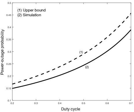
Figure 4: Power-outage probability versus duty cycle.

The the upper bound on the power-outage probability in Lemma 5 for the network with dense PBs is evaluated in Fig. 4 plotting the probability against the duty cycle $D$. The derived bound is found to be tight. Furthermore, the power-outage probability is observed to grow with increasing $D$ and converge to $0$ as $D$ approaches $0$. The reason is that large $D$ means that more time is spent on backscattering and less on energy harvesting, reducing the amount of harvested energy for operating the node circuits. The bound is also found to be tight by varying the circuit power consumption and reflection coefficient. The corresponding simulation results are omitted for brevity.

Figure 5: Success probability versus SIR threshold for both the normal WP-BackCom network and the network with dense PBs (with and without thermal noise). For the case with noise, the noise variance is set as $-90$ dBm.

In Fig. 5, the success probability for backscatter communication is plotted against the SIR threshold $\theta$ (in dB) for both the normal WP-BackCom network and the network with dense PBs with and without considering the impact of thermal noise. The derived theoretic lower bound is also plotted for comparison. One can see that deploying dense PBs substantially increases the success probability by reducing the likelihood of power outage. Moreover, the theoretic bounds on the success probability are observed to be tight for both networks. Fig. 5 also illustrates the effects of the thermal noise on success probability. One can see that the simulation results with (circle points) and without noise (solid lines) are close to each other, which validates the assumption of interference limited network.

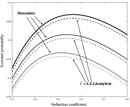
(a) Effect of the reflection coefficient

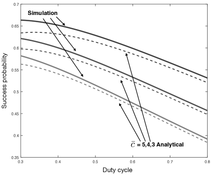
(b) Effect of the duty cycle

Figure 6: The effects of the backscatter parameters, namely the reflection coefficient and duty cycle, on the success probability for the normal WP-BackCom network with a variable expected number of backscatter nodes per cluster, $\bar{c}\in\{3,4,5\}$.

The curves of success probability versus the duty cycle and reflection coefficient are plotted in Fig. 6 for different values of $\bar{c}$. The curves based on the analytical results in Theorem 1 are plotted for comparison. It is observed that the theoretical lower bounds are tight. The curves show that the success probability is the concave function of the reflection coefficient, which is consistent with the discussion in Remark 7. The optimal value for the reflection coefficient is observed to be about $0.5-0.6$. Consider duty cycle $D$ in Fig. 6(b), the success probability reduces with increasing $D$. It is intuitive to understand because larger $D$ results in higher density of interference and larger power-outage probability. Furthermore, the lower bounds are not very tight when the value of $D$ is small. The reason is that smaller $D$ leads to higher receive power and transmission probability at receiver, using $\frac{\beta P_{c}}{1-\beta D}$ to replace $P_{t}$ (for obtaining the lower bound) incurs a little larger gap.

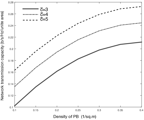
Figure 7: The network transmission capacity versus the PB density for the normal WP-BackCom network with a variable expected number of backscatter nodes per cluster, $\bar{c}\in\{3,4,5\}$

The curves of network transmission capacity versus the PB density are shown in Fig. 7 for different values of $\bar{c}$. When the density of PB is relatively small (e.g., $\lambda_{\text{pb}}\in[0.1,0.25]$) , the network capacity is observed to grow linearly with the PB density. This is aligned with theoretic result in Section V for the regime of almost-full network coverage. For a large PB density, the capacity saturates as the network becomes dense and interference limited. The linear relation no longer holds since the success probability no longer be approximated as $1$. In addition, it can be observed from Fig. 7 where increasing $\bar{c}$ contributes an approximately constant capacity gain insensitive to changes on the PB density.

Last, the effects of the backscatter parameters, namely the reflection coefficient $\beta$ and duty cycle $D$, on the network transmission capacity are shown in Fig. 8 for different values of $\bar{c}$. From Fig. 8(a), it can be observed that the capacity is a convex function of the duty cycle, which confirms Remark 8. The optimal duty cycle is almost identical (about $0.62$) for different values of $\bar{c}$. Furthermore, the capacity grows with the increasing node density and the gain is the largest at $D\approx 0.62$. Consider the curves of capacity versus reflection coefficient in Fig. 8(b). For $\beta$ larger than $0.3$ core, the capacity decreases rapidly as $\beta$ increases due to growing power-outage probability. This range of $\beta$ corresponds to almost-full network coverage and the observation is consistent with Remark 10.

(a) Effect of the duty cycle given reflection coefficient $\beta=0.6$

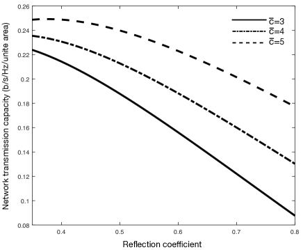
(b) Effect of the reflection coefficient given duty cycle $D=0.4$

Figure 8: The effects of the duty cycle and reflection coefficient on the network transmission capacity for a variable expected number of backscatter nodes per cluster, $\bar{c}\in\{3,4,5\}$.

VII Conclusion

In this work, we have proposed the new network architecture, namely the WP-BackCom network, for realizing dense backscatter communication networks using WPT enabled by PBs. A large-scale WP-BackCom network has been modeled using the PCP. Applying stochastic geometry theory, the success probability and the network transmission capacity have been derived to quantify the performance of network coverage and capacity, respectively. In particular, the results relate the network performance to the backscatter parameters, namely the duty cycle and the reflection coefficient.

The current work can be extended in several directions. In this work, each PB serves only a single node assuming beamforming. However, PB with isotropic transmission can serve multiple nodes, which makes the network-performance analysis more challenging but can lead to new insight into WP-BackCom network design. Next, following a similar approach as in this work, other types of backscatter communication networks, such as those based on UWB or ambient RF energy harvesting, can be modeled and studied using stochastic geometry comprising a wide range of spatial point processes including cluster point processes other than PCP, e.g., Gauss poisson processes and repulsive point processes (Ginibre point processes). Last, re-generated interference arising from backscattering interference by nodes is omitted in the current work. It is interesting and also important to investigate the effect of interference regeneration on the network performance.

-A Proof of Lemma 1

Let $\mathsf{E}_{\Phi}$ denote the expectation with respect to a random process/variable $\Phi$. Consider the typical cluster of the transmitting node process. Given the typical receiver located at $z\in\mathds{R}^{2}$, the characteristic functional of the intra-cluster interference in (8) is obtained as

$$\mathsf{E}\left[e^{-sI_{a}}\right] =\mathsf{E}_{\mathcal{N}_{0}\backslash\{X_{0}\},Y_{0}}\Bigg{[}\exp\Bigg{(}-s\sum\limits_{X\in\mathcal{N}_{0}\backslash\{X_{0}\}}\beta h_{X}\ell(|X-Y_{0}|^{-\alpha_{1}})|X\!-\!z|^{-\alpha_{2}}\Bigg{)}\Bigg{]}$$

$$\overset{(a)}{=}\mathsf{E}_{\mathcal{N}_{0},Y_{0}}\Bigg{[}\exp\Bigg{(}-s\sum\limits_{X\in\mathcal{N}_{0}}\beta h_{X}\ell(|X-Y_{0}|^{-\alpha_{1}})|X\!-\!z|^{-\alpha_{2}}\Bigg{)}\Bigg{]}$$

$$\overset{(b)}{=}\mathsf{E}_{Y_{0}}\Bigg{[}\exp\Bigg{(}-\bar{c}D\int\limits_{\mathds{R}^{2}}\Big{(}1-\mathsf{E}_{h}\Big{(}\exp\Big{(}-s\beta h\ell(|x-Y_{0}|^{-\alpha_{1}})|x-z|^{-\alpha_{2}}\Big{)}\Big{)}\times$$

$$\qquad\qquad\qquad f(|x-Y_{0}|)dx\Bigg{)}\Bigg{]}$$

$$=\mathsf{E}_{Y_{0}}\Bigg{[}\exp\Bigg{(}\!\!-\bar{c}D\int\limits_{\mathds{R}^{2}}\frac{1}{1+\frac{1}{s\beta\ell(|x-Y_{0}|^{-\alpha_{1}})|x-z|^{-\alpha_{2}}}}f(|x-Y_{0}|)dx\Bigg{)}\Bigg{]}$$

$$=\mathsf{E}_{Y_{0}}\Bigg{[}\exp\Bigg{(}\!\!\!-\bar{c}D\int\limits_{\mathds{R}^{2}}\frac{1}{1+\frac{1}{s\beta\ell(|x|^{-\alpha_{1}})|x+Y_{0}-z|^{-\alpha_{2}}}}f(|x|)dx\Bigg{)}\Bigg{]},$$ (42)

where $(a)$ and $(b)$ are obtained by applying Slivnyak’s Theorem an Campbell’s Theorem (see e.g., Chapter 4.5 in [32]), respectively. Using the PDF $f(\cdot)$ in (1) and (2) and the circuit-constraint function $\ell(\cdot)$ defined before (3), the desired result follows.

-B Proof of Lemma 2

By applying Slivnyak’s Theorem, the characteristic functional of the inter-cluster interference $I_{b}$ in (9) is obtained as

$$\mathsf{E}\left[e^{-sI_{b}}\right] =\mathsf{E}\Bigg{[}\exp\Bigg{(}-s\sum_{Y\in\Pi_{\text{pb}}}\sum_{X\in\mathcal{N}_{Y}}\beta h_{X}\ell(|X-Y|^{-\alpha_{1}})|X-z|^{-\alpha_{2}}\Bigg{)}\Bigg{]}$$

$$=\mathsf{E}\Bigg{[}\prod_{Y\in\Pi_{\text{pb}}}\mathsf{E}\Bigg{[}\exp\Big{(}-s\sum_{X\in\mathcal{N}_{Y}}\beta h_{X}\ell(|X-Y|^{-\alpha_{1}})|X-z|^{-\alpha_{2}}\Big{)}\Bigg{]}\Bigg{]}.$$

The inner expectation focusing on a single cluster can be derived using similar steps as in the proof of Lemma 1. As a result,

$$\mathsf{E}\left[e^{-sI_{b}}\right] =\mathsf{E}\Bigg{[}\exp\Bigg{(}-\sum_{Y\in\Pi_{\text{pb}}}\bar{c}Dq(s,Y,z)\Bigg{)}\Bigg{]}.$$ (43)

where $q(\cdot)$ is defined in Lemma 1. Applying Campbell’s Theorem gives the desired result.

-C Proof of Lemma 3

Using the definition of $I^{{}^{\prime}}$ in (15) and applying Slivnyak’s Theorem,

$$\mathsf{E}[e^{-sI^{{}^{\prime}}}] =\mathsf{E}\Big{[}\exp\Big{(}-s\beta\sum_{X\in\Pi_{\text{nd}}\backslash\{X_{0}\}}\Big{(}\sum_{Y\in\mathcal{N}_{X}}\eta g|Y-X|^{-\alpha_{1}}\Big{)}h_{X}|X-z|^{-\alpha_{2}}\Big{)}\Big{]}$$

$$=\mathsf{E}\Big{[}\prod_{X\in\Pi_{\text{nd}}\backslash\{X_{0}\}}\exp\Big{(}-s\beta\Big{(}\sum_{Y\in\mathcal{N}_{X}}\eta g|Y-X|^{-\alpha_{1}}\Big{)}h_{X}|X-z|^{-\alpha_{2}}\Big{)}\Big{]}$$

$$\overset{(a)}{=}\exp\Big{(}-\lambda_{\text{nd}}D\int_{\mathds{R}^{2}}\Big{(}1-\mathsf{E}_{\mathcal{N}_{X}}\mathsf{E}_{h}\Big{[}\exp\Big{(}-s\beta\Big{(}\sum_{Y\in\mathcal{N}_{X}}\eta g|Y-x|^{-\alpha_{1}}\Big{)}h|x-z|^{-\alpha_{2}}\Big{)}\Big{]}\Big{)}dx\Big{)}$$

$$\overset{(b)}{=}\exp\Big{(}-\lambda_{\text{nd}}D\int_{\mathds{R}^{2}}\Big{(}1-$$

$$\leavevmode\nobreak\ \leavevmode\nobreak\ \leavevmode\nobreak\ \leavevmode\nobreak\ \leavevmode\nobreak\ \leavevmode\nobreak\ \leavevmode\nobreak\ \leavevmode\nobreak\ \exp\Big{(}-2\pi\bar{m}\int_{0}^{\infty}\Big{(}1-\mathsf{E}_{h}\Big{[}\exp\Big{(}-s\beta\eta gh|x-z|^{-\alpha_{2}}r^{-\alpha_{1}}\Big{)}\Big{]}\Big{)}f(r)rdr\Big{)}\Big{)}dx\Big{)}$$

$$=\exp\Big{(}-\lambda_{\text{nd}}D\int_{\mathds{R}^{2}}\Big{(}1-\exp\Big{(}-2\pi\bar{m}\int_{0}^{\infty}\frac{1}{1+(s\beta\eta g)^{-1}r^{\alpha_{1}}|x-z|^{\alpha_{2}}}f(r)rdr\Big{)}\Big{)}dx\Big{)}$$ (44)

where both (a) and (b) are obtained by applying Campbell’s Theorem. The desired result follows.

-D Proof of Lemma 5

For the bound on the power-outage probability in (22), the term $\sum^{N}_{n}d_{n}^{-\alpha_{1}}$ is a compound Poisson process (or equivalently a shot-noise process) . Then using the result in (22) and the characteristic functional of a shot-noise process (see e.g., [16]),

$$p_{0}^{\prime} =\min_{\mu>0}\Big{\{}\exp\Big{(}\frac{\mu P_{c}}{(1-\beta D)\eta g}-2\pi\bar{m}\int^{\infty}_{0}\Big{(}1-e^{-\mu t^{-\alpha_{1}}}\Big{)}f(t)tdt\Big{)}\Big{\}}.$$ (45)

Note that the function of $\mu$to be minimized is convex. Thus the optimal value of $\mu$, denoted as $\mu^{*}$, can be found by solving the equation from setting the derivative of the said function as zero, yielding the result in the lemma statement.

References

- [1] K. Huang and X. Zhou, “Cutting last wires for mobile communication by microwave power transfer,” IEEE Commun. Mag., vol. 53, pp. 86 – 93, June 2015.
- [2] S. Bi, C. Ho, and R. Zhang, “Wireless powered communication: opportunities and challenges,” IEEE Commun. Mag., vol. 53, pp. 117 – 125, Apr. 2014.
- [3] C. Boyer and S. Roy, “Backscatter communication and RFID: Coding, energy, and MIMO analysis,” IEEE Trans. Commun., vol. 62, pp. 770 – 785, Mar. 2014.
- [4] K. Huang and V. Lau, “Enabling wireless power transfer in cellular networks: Architecture, modelling and deployment,” IEEE Trans. Wireless Commun., vol. 13, pp. 902–912, Feb. 2014.
- [5] H. Stockman, “Communication by means of reflected power,” in Proc. IRE, vol. 36, pp. 1196–1204, Oct. 1948.
- [6] T. Umeda, H. Yoshida, S. Sekine, Y. Fujita, T. Suzuki, and S. Otaka, “A 950-MHz rectifier circuit for sensor network tags with 10-m distance,” IEEE J. Solid State Circuits, vol. 41, pp. 35–41, Jan. 2006.
- [7] V. Chawla and D. Ha, “An overview of passive RFID,” IEEE Comm. Mag., vol. 45, pp. 11–17, Sep. 2007.
- [8] G. Yang, C. Ho, and Y. Guan, “Multi-antenna wireless energy transfer for backscatter communication systems,” (online) Available: http://arxiv.org/pdf/1503.04604v1.pdf, 2015.
- [9] J. Wang, H. Hassanieh, D. Katabi, and P. Indyk, “Efficient and reliable low-power backscatter networks,” in Proc. ACM SIGCOMM, pp. 61–72, 2012.
- [10] W. Saad, X. Zhou, Z. Han, and H. Poor, “On the physical layer security of backscatter wireless systems,” IEEE Trans. Wireless Commun., vol. 13, pp. 3442–3451, Jun. 2014.
- [11] J. Kimionis, A. Bletsas, and J. Sahalos, “Increased range bistatic scatter radio,” IEEE Trans. Commun., vol. 62, pp. 1091–1104, Mar. 2014.
- [12] D. Dardari, R. Errico, C. Roblin, A. Sibille, and M. Win, “Ultrawide bandwidth RFID: The next generation?,” Proc. of the IEEE, vol. 98, pp. 1570–1582, Sep. 2010.
- [13] V. Liu, A. Parks, V. Talla, S. Gollakota, D. Wetherall, and J. Smith, “Ambient backscatter: wireless communication out of thin air,” in Proc. ACM SIGCOMM, pp. 39–50, 2013.
- [14] B. Kellogg, A. Parks, S. Gollakota, J. Smith, and D. Wetherall, “Wi-Fi backscatter: internet connectivity for RF-powered devices,” in Proc. of the ACM SIGCOMM, pp. 607–618, 2014.
- [15] V. Liu, V. Talla, and S. Gollakota, “Enabling instantaneous feedback with full-duplex backscatter,” in Proc. of the ACM MobiCom, pp. 67–78, 2014.
- [16] M. Haenggi, J. Andrews, F. Baccelli, O. Dousse, and M. Franceschetti, “Stochastic geometry and random graphs for the analysis and design of wireless networks,” IEEE J. of Sel. Areas in Commun., vol. 27, pp. 1029–1046, Jul. 2009.
- [17] R. Ganti and M. Haenggi, “Interference and outage in clustered wireless Ad Hoc networks,” IEEE Trans. Info. Theory, vol. 9, pp. 4067–4086, Sep. 2009.
- [18] K. Gulati, B. Evans, J. Andrews, and K. Tinsley, “Statistics of co-channel interference in a field of poisson and poisson-poisson clustered interferers,” IEEE Trans. Sig. Proc., vol. 58, pp. 6207–6222, Dec. 2010.
- [19] Y. Chun, M. Hasna, and A. Ghrayeb, “Modeling heterogeneous cellular networks interference using poisson cluster processes,” IEEE J. of Sel. Areas in Commun., vol. 33, pp. 2182–2195, Oct. 2015.
- [20] V. Suryaprakash, J. Moller, and G. Fettweis, “On the modeling and analysis of heterogeneous radio access networks using a poisson cluster process,” IEEE Trans. Wireless Commun., vol. 14, pp. 1035–1047, Feb. 2015.
- [21] M. Afshang, H. Dhillon, and P. Chong, “Modeling and performance analysis of clustered device-to-device networks,” IEEE Trans. on Wireless Comm., pp. 4957–4972, Apr. 2016.
- [22] Y. Che, L. Duan, and R. Zhang, “Spatial throughput maximization of wireless powered communication networks,” IEEE J. of Sel. Areas in Commun., vol. 33, pp. 1534–1548, Aug. 2015.
- [23] I. Krikidis, “Simultaneous information and energy transfer in large-scale networks with/without relaying,” IEEE Trans. Commun., vol. 62, pp. 900–912, Mar. 2014.
- [24] P. Mekikis, A. Lalos, A. Antonopoulos, L. Alonso, and C. Verikoukis, “Wireless energy harvesting in two-way network coded cooperative communications: a stochastic approach for large scale networks,” IEEE Commun. Letters, vol. 18, pp. 1011–1014, Jun. 2014.
- [25] H. Dhillon, Y. Li, P. Nuggehalli, Z. Pi, and J. Andrews, “Fundamentals of heterogeneous cellular networks with energy harvesting,” IEEE Trans. on Wireless Comm., vol. 13, pp. 2782–2797, Apr. 2014.
- [26] A. Sakr and E. Hossain, “Cognitive and energy harvesting-based D2D communication in cellular networks: Stochastic geometry modeling and analysis,” IEEE Trans. Commun., vol. 63, pp. 1867–1880, Mar. 2015.
- [27] X. Lu, I. Flint, D. Niyato, N. Privault, and P. Wang, “Self-sustainable communications with RF energy harvesting: Ginibre point process modeling and analysis,” IEEE J. of Sel. Areas in Commun., vol. 34, pp. 1518–1535, Apr. 2016.
- [28] U. Karthaus and M. Fischer, “Fully integrated passive UHF RFID transponder IC with 16.7- mu;W minimum RF input power,” IEEE J. of Solid-State Circuits., vol. 38, pp. 1602–1608, Oct 2003.
- [29] S. Weber, J. Andrews, and N. Jindal, “An overview of the transmission capacity of wireless networks,” IEEE Trans. Commun., vol. 58, pp. 3593–3604, Dec. 2010.
- [30] F. Baccelli, B. Blaszczyszyn, and P. Muhlethaler, “An ALOHA protocol for multihop mobile wireless networks,” IEEE Trans. on Info. Theory, vol. 52, pp. 421–36, Feb. 2006.
- [31] J. Andrews, F. Baccelli, and R. Ganti, “A tractable approach to coverage and rate in cellular networks,” IEEE Trans. Commun., vol. 59, pp. 3122–3134, Nov. 2011.
- [32] M. Haenggi, Stochastic geometry for wireless networks. Cambridge University Press, 2012.