Bounding the persistency of the nonlocality of W states

Abstract

The nonlocal properties of the W states are investigated under particle loss. By removing all but two particles from an $N$-qubit W state, the resulting two-qubit state is still entangled. Hence, the W state has high persistency of entanglement. We ask an analogous question regarding the persistency of nonlocality introduced in [Phys. Rev. A 86, 042113]. Namely, we inquire what is the minimal number of particles that must be removed from the W state so that the resulting state becomes local. We bound this value in function of $N$ qubits by considering Bell nonlocality tests with two alternative settings per site. In particular, we find that this value is between $2N/5$ and $N/2$ for large $N$. We also develop a framework to establish bounds for more than two settings per site.

I Introduction

Entanglement and nonlocality are two manifestations of quantum correlations, both are essential ingredients of quantum theory. They also play an important role in the field of quantum information nielsenchuang . For instance, entanglement is in the heart of quantum teleportation and plays a crucial role in quantum algorithms horodecki ; geza . Nonlocality, on the other hand, witnessed by the violation of Bell inequalities bell , reduces communication complexity buhrmanreview ; buhrman and enables device-independent quantum information protocols bellreview ; valerio . These protocols do not rely on a detailed knowledge of the internal working of the experimental devices used, thereby allowing secure cryptography involving untrusted devices qkd or expansion of secure random numbers random1 ; random2 .

The quantification of entanglement and nonlocality in the bipartite case (i.e., the case when two parties share an entangled state) is relatively well understood. However, the multipartite case is much less explored. This is mainly due to the rapidly growing complexity of the problem with the number of parties. For instance, for bipartite pure states, there is a unique measure of entanglement, however, for three or more parties, this is not true any more (see e.g., Refs. plenio ; szalay ). Concerning nonlocality, there is a single tight Bell inequality for two binary settings per party, the Clauser-Horne-Shimony-Holt (CHSH) one bell ; chsh . However, moving to three parties, the number of tight Bell inequalities already becomes 42 sliwa . In fact, determining all Bell inequalities for growing number parties is an NP-hard problem pitowski ; NP . Bipartite and tripartite quantum nonlocality are different from a fundamental point of view as well. While Gleason’s theorem can be extended to the bipartite scenario, however, there remains a gap between the quantum and Gleason’s correlations in the tripartite scenario acinObs .

One of the most famous multipartite quantum states is the W state Wstate playing a crucial role in the physics of the interaction between light and matter. Up to now, W states have been prepared in lots of experiments, e.g., photonic experiments can generate and characterize six qubit entangled states Wexp1 . More recently, genuine 28-particle entanglement was detected in a Dicke-like state (a generalization of the W state) in a Bose-Einstein condensate Wexp2 .

W states are very robust to losses, hence suited to quantum information applications such as quantum memories qmemory . For instance, by tracing out all but two parties from an $N$-party W state, the remaining two-qubit state is still entangled, no matter how big $N$ is. Hence, the W state shows a high persistency of entanglement against particle loss (actually, the highest possible persistency among $N$ qubit states buzek ).

On the other hand, one may wonder how robust the nonlocality of the W state is with respect to particle loss. In order to quantify this, Ref. persistency introduces the persistency of nonlocality of $N$-party quantum states $\rho$, $P_{NL}(\rho)$, which is the minimal number of particles to be removed for nonlocal quantum correlations to vanish. Ref. persistency investigates this measure for various classes of multipartite states including W states up to $N=7$ with two settings per site. In this paper, we bound this value both from above and from below for any $N$-qubit W states. To do this, we refine the definition of $P_{NL}(\rho)$ to account for Bell nonlocality involving $m$ settings per party. This quantity will be called $P_{NL}^{m}(\rho)$. Clearly, in the limit of large $m$, $P_{NL}^{m}(\rho)$ tends to $P_{NL}(\rho)$. Our main result concerns the case of $m=2$ and we prove the bounds of $2N/5\leq P_{NL}^{2}(W_{N})\leq N/2$ for $N$ large, featuring a relatively small gap between the upper and lower bounds. The lower bound is based on an explicit construction of a class of Bell inequalities. We also give a numerical framework to put reliable lower bounds on $P_{NL}^{m}(W_{N})$ beyond two settings (up to $m=6$) and a tractable number of $N$ parties. This numerical study supports that our analytical lower bounds for $P_{NL}^{2}(W_{N})$ are tight. There are recent papers which discuss the robustness of Dicke states dicke (and in particular the W state) to various types of noises rafael ; tomer ; sohbdi . Lower bounds also follow from these papers for the value of $P_{NL}^{2}(W_{N})$. In particular, we obtain considerable improvement over the lower bounds presented in Ref. tomer .

Notably, the persistency of nonlocality also gives a device-independent bound on the persistency of entanglement introduced in Ref. briegel . Other device-independent approaches to quantify multipartite entanglement including W states appeared in Refs. DIW ; tomoW ; numW . On the other hand, multipartite W states are promising candidates to close the detection loophole eberhard in multipartite Bell tests Wdetloophole . Such Bell violations would complement the experimental loophole-free violations obtained recently in the bipartite case loopholefree .

The structure of the paper is as follows. Section II introduces notation. Section III proves a simple upper bound on the persistency of nonlocality $P^{m}_{NL}$ for W states and in general for any permutationally symmetric state with two settings per party (case $m=2$). On the other hand, section IV presents lower bound values based on numerical investigations. To this end, we first outline the numerical method, then show results for $m=2$ and also beyond $m=2$ up to $m=6$. In section V, a family of Bell inequalities is presented (valid for any number of parties $N$), which allows us to obtain good lower bounds for $P_{NL}^{2}(W_{N})$. The paper ends with a discussion in section VI.

II Bell setup

Let us imagine the following Bell setup bell . A quantum state $\rho$ is shared between $n$ spatially separated systems, on which the local observers can conduct measurements. We focus on binary outcome measurements in which case we may define the joint correlators by the following set of expectation values:

$$\left\{\langle\mathcal{M}_{j_{1}}^{(1)}\ldots\mathcal{M}^{(n)}_{j_{n}}\rangle\right\}=\left\{\mathrm{Tr}{\left(\rho\mathcal{M}_{j_{1}}^{(1)}\otimes\ldots\otimes\mathcal{M}_{j_{n}}^{(n)}\right)}\right\}$$ (1)

with $j_{l}=0,1,\ldots,m$ and $l=1,\ldots,n$. We identify $\mathcal{M}_{0}^{(l)}=\leavevmode\hbox{\small 1\normalsize\kern-3.30002pt1}$ and $\mathcal{M}_{j_{l}}^{(l)}$ refers to the $j_{l}$th $\pm 1$-valued observable of party $l$. The corresponding real vector of correlators defines a point in the $(1+m)^{n}$ dimensional space of probabilities. Each member of the set (1) has an order, which is given by the amount of parties $o$ involving a non-trivial observable (i.e. not involving $\mathcal{M}_{0}^{(l)}=\leavevmode\hbox{\small 1\normalsize\kern-3.30002pt1}$). In particular, those with $o=n$ are usually called full-correlators, while those with $o=1$ are called one-body correlators or marginal terms.

A multipartite (2-outcome) Bell inequality bell is a linear function of the above correlators (1),

$$\sum_{j_{1}=0}^{m}\ldots\sum_{j_{n}=0}^{m}{\alpha_{j_{1},\ldots,j_{n}}}\langle\mathcal{M}_{j_{1}}^{(1)}\ldots\mathcal{M}^{(n)}_{j_{n}}\rangle\leq\beta_{c},$$ (2)

where we denote by $\beta_{c}$ the bound which holds for any local hidden variable model. These are the correlations which the parties can simulate by merely using local strategies and some shared classical information. The local correlations attainable this way forms a polytope, the so-called Bell polytope, whose extremal points consist of those vectors in (2) in which all correlators factorize, that is,

$$\langle\mathcal{M}_{j_{1}}^{(1)}\ldots\mathcal{M}^{(n)}_{j_{n}}\rangle=\langle\mathcal{M}_{j_{1}}^{(1)}\rangle\cdot\ldots\cdot\langle\mathcal{M}_{j_{n}}^{(n)}\rangle$$ (3)

and the mean value of each single party $\langle\mathcal{M}_{j_{l}}^{(l)}\rangle$, $(l=1,\ldots,n,j_{l}>0)$ equals either $-1$ or $+1$. Let us define the persistency of nonlocality of a multipartite state $\rho$ according to Ref. persistency as follows. Let us take the partial trace over $0<k<N$ systems $i_{1},...,i_{k}\in\{1,...,N\}$, and denote the $n=N-k$-party reduced state by $\rho_{red}$. The persistency of nonlocality of $\rho$, $P_{NL}(\rho)$, is defined as the minimal $k$ such that the reduced state $\rho_{red}$ becomes local for at least one set of subsystems $i_{1},...,i_{k}$. In other words, the correlators (1) obtained from local measurements $\mathcal{M}_{j_{l}}^{(l)}$ on $\rho_{red}$ do not violate any Bell inequality.

If we allow at most $m$ different measurement settings in the Bell expression (2), we arrive at $P^{m}_{NL}(\rho)$ which provides a lower bound to $P_{NL}(\rho)$ and for $m\rightarrow\infty$ recovers $P_{NL}(\rho)$.

In this paper, we focus on computing $P^{m}_{NL}(\rho)$ for the noiseless $N$-qubit W state Wstate , $\rho=|W_{N}\rangle\langle W_{N}|$, where

$$|W_{N}\rangle=\frac{1}{\sqrt{N}}\left(|0\ldots 01\rangle+|0\ldots 10\rangle+\ldots+|10\ldots 0\rangle\right).$$ (4)

We may consider this state as a state of an atomic ensemble, and we assume that $k$ particles are lost from this ensemble. In that case, the reduced state contains $n=N-k$ particles, and the density matrix reads

$$\rho(N,k)=\frac{n}{N}|W_{n}\rangle\langle W_{n}|+\frac{k}{N}|0^{\otimes n}\rangle\langle 0^{\otimes n}|.$$ (5)

Since the W state is permutationally symmetric, the reduced state $\rho(N,k)$ does not depend on the particular set of subsystems removed, which simplifies considerably the analysis of $P_{NL}^{m}(W_{N})$.

In the next section we provide an upper bound of $N/2$ for $P_{NL}^{m=2}(W_{N})$ in case of arbitrary even $N$ number of parties, whereas in Sec. IV we bound this quantity by $2N/5$ from below.

III An upper bound for the persistency of nonlocality of the W state

We first prove the following lemma:

Lemma 1.

Let us have a $2n$-qudit permutationally invariant state, $\rho\in({\mathbb{C}}^{d})^{\otimes 2n}$, where $d\geq 2$ and $n\geq 1$. By tracing out any $n$ qudits, the remaining $n$-qudit system $\rho_{red}\in({\mathbb{C}}^{d})^{\otimes n}$ cannot violate any two-setting $n$-party Bell inequality with arbitrary number of outcomes.

Proof.

We take $N=2n$ and denote the $n$-qudit reduced state of an $N$-qudit permutationally invariant state $\rho$ by $\rho_{red}$ and the two measurements conducted on station $l\in\{1,\ldots,n\}$ by $M^{(l)}_{a_{l}|j_{l}}$, where $j_{l}=1,2$. By permutationally invariance we mean that the exchange of any two qudits of the $N$-qudit state $\rho$ does not change the state itself. Then, the $n$-particle joint probability distribution reads

$$P(a_{1},a_{2},...,a_{n}|j_{1},j_{2},...,j_{n})$$

$$=\mathrm{Tr}\left(\rho_{red}\mathcal{M}^{(1)}_{a_{1}|j_{1}}\otimes\mathcal{M}^{(2)}_{a_{2}|j_{2}}\ldots\otimes\mathcal{M}^{(n)}_{a_{n}|j_{n}}\right),$$ (6)

It is not difficult to see that the same probability distribution can be achieved in the following way: Let us redistribute the permutationally invariant state $\rho$ between $n$ parties such that the $l$th qudit pair $(l,l+n)$ belongs to party $l\in\{1,\ldots,n\}$ (so that each party owns two qudits). Then party $l$ performs measurement $\mathcal{M}^{(l)}_{a_{l}|j_{l}=1}$ on the first qudit and measurement $\mathcal{M}^{(l)}_{a_{l}|j_{l}=2}$ on the second qudit of the $l$th pair. This generates the same distribution as of Eq. (III). Since for any $l$ these two measurements act on different subspaces, they are commuting. However, Bell inequality violation is not possible (with any number of outcomes) if the two alternative measurements for each party are pairwise commuting terhal . ∎

Since the W state is a permutationally invariant multiqubit state (with local dimension $d=2$), Lemma 1 above directly applies to our situation, hence we get the upper bound $P_{NL}^{m}(W_{N})\leq n$ for $m=2$ with $N=2n$. In other words, $P_{NL}^{2}(W_{N})\leq N/2$ for even $N$.

Some notes are in order. (i) It is straightforward to extend Lemma 1 to more than two settings as well. For multiple settings, we get the general upper bound $P_{NL}^{m}(W_{N})\leq(m-1)n$ with $N=mn$. However, we conjecture that these upper bounds are not tight in general. For $m=2$, a gap between the lower and upper bound values for the $6\leq N\leq 20$-qubit W states are supported by a numerical study performed in Sec. IV. For $m$ infinite, the trivial upper bound $P_{NL}(W_{N})\leq N-1$ follows by plugging $n=1$ in the above formula. If this bound happened to be tight, it would imply that the two-qubit reduced state $\rho_{red}=(2/N)|\psi^{+}\rangle\langle\psi^{+}|+(1-(2/N))|00\rangle\langle 00|$ of the $W_{N}$ state was Bell nonlocal. For large $N$ this is very unlikely, since the weight of the entangled part $|\psi^{+}\rangle\langle\psi^{+}|$ goes to zero. In fact, a recent computer study in Ref. nagy suggests that the state $\rho(p)=p|\psi^{+}\rangle\langle\psi^{+}|+(1-p)|00\rangle\langle 00|$ is local for $p<1/\sqrt{2}$. Similarly, A. Amirtham conjectures in Ref. ami that the state $\rho(p)$ is local for $p<2/3$.

(ii) The permutational invariance property of the state is crucial in the above state. If the multipartite state does not possess this high symmetry, e.g. it only obeys translational invariance, the above theorem does not hold true any more. Let us illustrate this with a simple example. We consider a 4-qubit translationally invariant state $|\psi\rangle=|\psi^{+}\rangle_{13}|\psi^{+}\rangle_{24}$, where $|\psi^{+}\rangle_{ij}=(|0\rangle_{i}|1\rangle_{j}+|1\rangle_{i}|0\rangle_{j})/\sqrt{2}$. Let us trace out particles $2$ and $4$ (constituting half of the 4 particles), and as a result we get a maximally entangled pair of qubits, which violates maximally the bipartite CHSH-Bell inequality chsh . Nevertheless, translationally invariant systems also impose certain restrictions which can be exploited in Bell scenarios as studied in Ref. Oliveira .

IV A lower bound for the persistency of nonlocality of the W state

We now give a numerical procedure which allows us to get useful (and often tight) lower bounds to $P_{NL}^{m}(W_{N})$. We note that this procedure with some modification can also be applied to generic permutationally invariant multiqubit states.

We consider the Bell violation of the following one-parameter family of states:

$$\rho(n,p)=(1-p)|W_{n}\rangle\langle W_{n}|+p|0^{\otimes n}\rangle\langle 0^{\otimes n}|.$$ (7)

Notice that the state (7) reproduces (5) with $p=k/N$. Hence, given an $n$-party $m$-setting Bell inequality which is violated by state (7) with a given critical value, $p_{crit}$, we get the following lower bound on the persistency:

$$P_{NL}^{m}(W_{N})=N-n+1,$$ (8)

where $N=\lfloor n/(1-p_{crit})\rfloor$, where $\lfloor x\rfloor$ maps a real number $x$ to the largest previous integer. Hence, in order to get good lower bounds to $P_{NL}^{m}(W_{N})$ our task reduces to get good upper bounds to $p_{crit}$. To this end, we introduce the following linear programming based numerical method.

Let us stick to $m=2$ settings (generalization to more settings is straightforward). For simplicity we assume that all parties measure the same qubit observables, that is, $\mathcal{M}^{(1)}_{j}=\mathcal{M}^{(2)}_{j}=\ldots=\mathcal{M}^{(n)}_{j}$ for $j=1,2$. Moreover, due to symmetry of the states, we assume these observables are coplanar, lying on the $X-Z$ equatorial plane. Other works (e.g., Refs. otherW ; structure ; tomoW ) maximizing Bell functionals using the W state rely on the same symmetry considerations. With this simplification, we have two optimization parameters. Hence, for the state $W_{n}$ and the above measurements, the $(1+m)^{n}=3^{n}$-dimensional correlation point $P_{1}$ given by the set of correlators (1) is defined by two angles. Likewise, we define the correlation point $P_{0}$ generated by the same measurements and the state $\rho=|0^{\otimes n}\rangle\langle 0^{\otimes n}|$ in Eq. (1). Geometrically, the correlations accessible in a local hidden variables theory form a polytope, the so-called Bell polytope, with vertices defined by deterministic classical strategies for a fixed scenario of $n$ parties and $m$ settings (see Ref. bellreview for a review). The two correlation points $P_{0}$ and $P_{1}$ are situated within this space. Since the product state $|0^{\otimes n}\rangle\langle 0^{\otimes n}|$ is local, point $P_{0}$ sits inside the Bell polytope, whereas point $P_{1}$ depends on the two measurement angles and may well fall outside the Bell polytope (see Fig. 1). For a given $p$ in (7), the corresponding correlation point is $(1-p)P_{1}+pP_{0}$, and $p_{crit}$ is given by the intersection of the line joining points $P_{0}$ and $P_{1}$ with the boundary of the polytope (see Figure 1). Given the two measurement angles, standard linear programming allows us to compute $p_{crit}$ and the underlying facet, which corresponds to a Bell inequality.

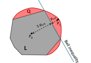
Figure 1: A schematic view of the Bell polytope (region L) and the space attainable with quantum systems (region Q). The correlation point $P_{1}$ corresponding to the $W_{N}$ state is outside the Bell polytope, whereas the point $P_{0}$ corresponding to the product state falls inside the Bell polytope. $p_{crit}$ is fully determined by points $P_{0},P_{1}$ and the facets of the polytope.

Clearly, the above described procedure works for $m>2$ as well. In particular, we have chosen a given Bell scenario ($n$ parties, $m$ settings) and by varying the $m$ angles, we maximized the value of $p_{crit}$. We note that this search is a heuristic one and as such it is not guaranteed to terminate in a global maximum of $p_{crit}$. However, the obtained value still defines a lower bound to $P^{m}_{NL}$ in (8). The critical $p$ values obtained in function of $n$ and $m$ are displayed in Fig. 2. We may observe that, as $m$ increases, the affordable number of parties $n$ decreases. For the simplest case of $m=2$, numerically we could afford $n=14$. In addition, we had to resort to a symmetrization procedure of the Bell polytope introduced in JD which considerably reduces the complexity of the problem in order to attain $n=14$.

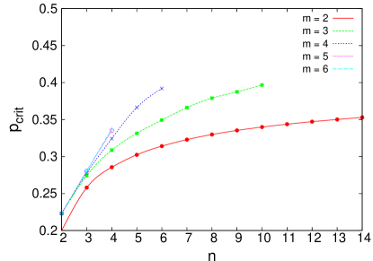
Figure 2: For $\rho(n,p)$ states of $n$ qubits (7), the graph shows lower bounds on the threshold probability $p_{crit}$ obtained using our numerical method up to $m=6$ measurement settings.

Plugging the $p_{crit}$ values shown in Fig. 2 into formula (8), we get Table 1, where the computed persistencies $P_{NL}^{m}$ are shown for $m\leq 6$. This way we get entries in the table only for $N$ satisfying $N=\lfloor n/(1-p_{crit})\rfloor$, but a slight modification allows us to obtain numbers for any $N$ parties: Fix $N$, and choose the largest $k$ integer such that $p_{crit,n-k}>k/N$, where $p_{crit,n-k}$ stands for $p_{crit}$ evaluated by the number of parties $n-k$. Then a lower bound on the persistency $P_{NL}^{m}$ for the $N$-qubit W state is given by $P_{NL}^{m}=k+1$.

N	$m=2$	$m=3$	$m=4$	$m=5$	$m=6$
2	1	1	1	1	1
3	1	1	1	1	1
4	2	2	2	2	2
5	2	2	2	2	2
6	2	2	2	3	3
7	3	3	3
8	3	3	3
9	3	4	4
10	4	4
11	4	5
12	4	5
13	5	5
14	5	6
15	6	6
16	6	7
17	6
18	7
19	7
20	8

Table 1: Lower bound values for persistency of nonlocality $P_{NL}^{m}$ for the $W_{N}$ state with $m=2,\ldots,6$ binary-outcome measurement settings per party. The results are based on the numerical method described in the text.

In Table 1, for $m=2$, the first entries $N=2,3,\ldots,7$ match the numbers from previous study persistency . However, by fixing $N$ and going to higher number of settings $m$ sometimes we get a higher persistency of nonlocality. For instance, in case of $N=6$ parties, $P_{NL}^{5}=3$, which is to be compared to $P_{NL}^{2}=2$. For $m=2$, we extracted the optimal Bell inequalities corresponding to $p_{crit}$ for various $n$ values. For $n$ even, a common structure has been found. In fact, they turned out to be members of a family of Bell inequalities valid for any $n$ even. Details of this class of inequalities are presented in Sec. V. We optimized the quantum value of these inequalities in function of the two measurement angles. Fig. 3 shows results for $p_{crit}$ up to $n=50$ of this family. We also show results using the ansatz that the two measurement settings are $Z$ and $X$, in which case $p_{crit}=(2n-4)/(5n-2)$ for $n$ even. According to the figure, for larger $n$ the $(Z,X)$ pair of settings become close to optimal. The $p_{crit}$ values have been also studied in Ref. tomer for specific families of known Bell inequalities from the literature, with the best lower bound values coming from the WWWZB inequalities WWWZB . For comparison, these $p_{crit}$ values are displayed. For $n=50$, $p_{crit}=0.3142$, which is suboptimal with respect to our $p_{crit}=(2n-4)/(5n-2)\simeq 0.3871$.

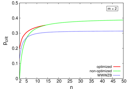
Figure 3: For $\rho(n,p)$ states of $n$ qubits (7), the graph shows lower bounds on the threshold probability $p_{crit}$ obtained using our numerical method for $m=2$ measurement settings. These bounds coincide with the bounds coming from our class of Bell inequalities for 2 measurement settings up to $n=14$ and we conjecture to be the same for any even $n$ particles. We show results for our Bell inequalities with optimized and non-optimized settings (in the latter case, the two observables are the Pauli operators $Z$ and $X$). The lower curve reproduces the results of Ref. tomer in case of the WWWZB inequalities WWWZB .

Finally, Fig. 4 shows the upper bound values due to section III and the lower bound values for $P^{2}_{NL}(W_{N})$ up to $N=50$ due to our Bell family. We conjecture that the exact value for $P^{2}_{NL}(W_{N})$ is defined by the lower curve (that is, no better Bell inequalities than our family in section V exist in this respect). For instance, the best lower bound for $P^{2}_{NL}(W_{N})$ so far comes from the WWWZB inequalities analyzed in Ref. tomer , which lies below our curve for the lower bound, and according to the conjecture in Ref. tomer it goes to $N/3$ in the limit of large $N$. On the other hand, our asymptotic lower bound value of $2N/5$ is considerable higher. It is also worth noting that the upper bound value on $P^{2}_{NL}$ shown in the figure holds true for any permutationally invariant $N$-qubit state. Hence, Dicke states with more than one excitation, as a notable subset of permutationally invariant states, cannot perform significantly better than $W$ states in the two-setting case.

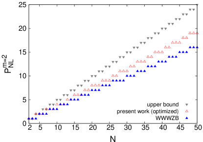
Figure 4: For $W$ states of $N$ qubits, the graph shows upper bounds (marked by a triangle pointing down) and lower bounds (marked by triangles pointing up) on the persistency of nonlocality $P_{NL}^{m=2}(W_{N})$.

In Ref. tomer , the Dicke states (including the $W_{N}$ state) were analyzed in terms of two decoherence models: loss of particles and loss of excitations. The first one relates to the measure $P_{NL}$ discussed in this paper, whereas the latter one is related to $p_{crit}$ in formula (7). Indeed, if we start from an $n$-qubit W state which is effected by a decoherence where in each mode an excitation has a probability $p$ of being lost, it brings the W state into (7). Appendix A shows a derivation of this result.

Next section gives all the details, including the quantum and local bounds, of our particular family of two-setting Bell inequalities providing $p_{crit}=(2n-4)/(5n-2)$ for even $n$. In case of large $n$, this goes to $2/5$ which we conjecture to be the largest achievable critical value among all two-setting Bell inequalities.

V A family of two-setting multipartite Bell inequalities

Standard form of permutationally symmetric Bell inequalities.– The Bell inequality to be considered consists of correlators (1) which are invariant under any permutation of the parties. By imposing the permutational symmetry, one requires that the expectation values $\langle\mathcal{M}_{j_{1}}^{(1)}\ldots\mathcal{M}^{(n)}_{j_{n}}\rangle$ and $\langle\mathcal{M}_{j_{1}}^{\sigma(1)}\ldots\mathcal{M}^{\sigma(n)}_{j_{n}}\rangle$ are the same, where $\sigma:\{1,\ldots,n\}\rightarrow\{\sigma(1),\ldots,\sigma(n)\}$ is an arbitrary permutation of the set $\{1,\ldots,n\}$. Let us denote by $S_{n}$ all permutations of the set $\{1,\ldots,n\}$. Then, it will be useful to define

$$S^{o}_{r}\equiv\sum_{\sigma\in S_{n}}\langle\mathcal{M}_{j_{1}}^{\sigma(1)}\ldots\mathcal{M}^{\sigma(n)}_{j_{n}}\rangle,$$ (9)

where the sum ranges over all permutations of the set $\{1,\ldots,n\}$. In $S^{o}_{r}$ above, $o$ is the order of correlators and $r$ is the number of $1$’s occurring in the list $\{j_{1},\ldots,j_{n}\}$. Let us now define the symmetrized correlation vector by the above ordered real vectors as follows

$$\vec{S}\equiv\{S^{o}_{r}\}^{o=1,\ldots,n}_{r=0,\ldots,o}.$$ (10)

In a similar way, we define the vector of coefficients associated with $\vec{S}$ as

$$\vec{\alpha}\equiv\{\alpha^{o}_{r}\}^{o=1,\ldots,n}_{r=0,\ldots,o}.$$ (11)

As a result, we arrive at the general form of a permutationally symmetric Bell inequality:

$$I\equiv\vec{\alpha}\cdot\vec{S}=\sum_{\begin{subarray}{c}{o=1,\ldots,n}\\ {r=0,\ldots,o}\end{subarray}}{\alpha^{o}_{r}S^{o}_{r}}\leq\beta_{c},$$ (12)

where $\beta_{c}$ is the local maximum, which holds for any local hidden variable model. It is worth noting that the WWWZB class WWWZB contains only full-correlator terms ($o=n$), whereas our construction of Bell inequalities turns out to contain all different orders, starting from marginal terms ($o=1$) up to full-correlation terms ($o=n$). There also exist permutationally symmetric $n$-party Bell inequalities involving only first and second order terms ($o=1,2$) twobody . The usefulness of these kind of inequalities in the particle loss model is an open and interesting question in our view.

As an illustrative example, let us discuss the case of 4 particles ($n=4$). In this case, $\vec{S}$ looks as follows

$$\vec{S}=\{S^{1}_{1},S^{1}_{0};S^{2}_{2},S^{2}_{1},S^{2}_{0};S^{3}_{3},S^{3}_{2},S^{3}_{1},S^{3}_{0};S^{4}_{4},S^{4}_{3},S^{4}_{2},S^{4}_{1},S^{4}_{0}\},$$ (13)

where we used semicolon (;) in order to separate components with different order $o$. By identifying $\mathcal{M}_{0}^{(l)}=1$, $l=1,\ldots,4$ and $\mathcal{M}_{j}^{(1)}=A_{j}$, $\mathcal{M}_{j}^{(2)}=B_{j}$, $\mathcal{M}_{j}^{(3)}=C_{j}$, $\mathcal{M}_{j}^{(4)}=D_{j}$ for $j=1,2$ in Eq. (9), we have the following mean values displayed for some particular cases (neglecting the mean value signs):

$$S^{1}_{1}= 6(A_{1}+B_{1}+C_{1}+D_{1}),$$

$$S^{2}_{2}= 4(A_{1}B_{1}+A_{1}C_{1}+A_{1}D_{1}+B_{1}C_{1}+B_{1}D_{1}+C_{1}D_{1}),$$

$$S^{2}_{0}= 4(A_{2}B_{2}+A_{2}C_{2}+A_{2}D_{2}+B_{2}C_{2}+B_{2}D_{2}+C_{2}D_{2}),$$

$$S^{3}_{1}= 2(A_{1}B_{2}C_{2}+A_{1}B_{2}D_{2}+A_{1}C_{2}D_{2})$$

$$+2(A_{2}B_{1}C_{2}+A_{2}B_{1}D_{2}+B_{1}C_{2}D_{2})$$

$$+2(A_{2}B_{2}C_{1}+A_{2}C_{1}D_{2}+B_{2}C_{1}D_{2})$$

$$+2(A_{2}B_{2}D_{1}+A_{2}C_{2}D_{1}+B_{2}C_{2}D_{1}),$$

$$S^{4}_{0}= 24A_{2}B_{2}C_{2}D_{2},$$ (14)

where we recall that $o$ denotes the order in the superindex of $S^{o}_{r}$, whereas $r$ is the number of occurrences of subindex 1 in $S^{o}_{r}$. For instance, $S^{3}_{1}$ above consists of all length-3 sequences from $A,B,C$ and $D$ letters with the occurrence of a single subindex 1.

The specific class of Bell inequalities.– Let us now give the explicit form of a Bell inequality $I$ defined by the vector of coefficients $\vec{\alpha}$ in Eq. (12). This family has been extracted from the numerical method of Sec. IV. In particular, we introduce a family of Bell inequalities $I_{n}$ valid for any even number of particles $n$ as follows

$$I_{n}\equiv\vec{\alpha}_{n}\cdot\vec{S}_{n}=\sum_{\begin{subarray}{c}{o=1,\ldots,n}\\ {r=0,\ldots,o}\end{subarray}}{\alpha^{o}_{r}S^{o}_{r}}\leq\beta_{c,n}.$$ (15)

The vector of coefficients $\vec{\alpha}=\{\alpha^{o}_{r}(o=1,\ldots,n,r=0,\ldots,o)\}$ reads as

$$\vec{\alpha}=\begin{cases}\alpha^{2k}_{0}=F_{k,n},&k=1,\ldots,n/2\\ \alpha^{2k-1}_{1}=G_{k,n}+2w_{n}\delta_{k,1},&k=1,\ldots,n/2\\ \alpha^{2}_{2}=-w_{n},\\ \alpha^{o}_{r}=0,&\text{otherwise}\end{cases}$$ (16)

where $\delta_{i,j}$ is the Kronecker delta (1 if $i=j$, 0 otherwise), and the functions entering eq. (16) above are

$$F_{k,n} =(-1)^{k}\frac{n-2}{2}(n+1-2k)\binom{n/2}{k},$$

$$G_{k,n} =(-1)^{k}\frac{n+2}{2}n\binom{n/2-1}{k-1},$$

$$w_{n} =\frac{n(n-1)(n+2)}{2^{4-n}\binom{n}{n/2}}.$$ (17)

Especially for $n=4$, our 4-party Bell inequality looks as follows:

$$I_{4}=12S^{1}_{1}-12S^{2}_{2}-6S^{2}_{0}+12S^{3}_{1}+S^{4}_{0}\leq 128,$$ (18)

where the middle terms appear explicitly in (V) and the local bound is due to formula (19) given in the next subsection for the general $n$-party case.

Local bound.– The local maximum, which is the maximum value one obtains using local resources only, is given by

$$\beta_{c,n}=n!\left(w_{n}-\frac{(n-2)(n+1)}{2}\right)$$ (19)

in case of any even number of particles $n$, where

$$w_{n}=\frac{n(n-1)(n+2)}{2^{4-n}\binom{n}{n/2}}.$$ (20)

We have checked the validity of the above local bound $\beta_{c,n}$ for $n\leq 16$ ($n$ even) by listing all possible deterministic strategies (i.e., vertices of the Bell polytope). These are the strategies for which all correlators factorize (see eq. 3) and each single party marginal $\langle\mathcal{M}_{j_{l}}^{(l)}\rangle$, $(l=1,\ldots,n,j_{l}=1,2)$ equals either $-1$ or $+1$. One of the above deterministic strategies, due to linearity of the Bell functional, will provide the local maximum. Notice that $\langle\mathcal{M}_{0}^{(l)}\rangle$, ($l=1,\ldots,n$) equals $+1$ by definition. Below we provide an analytical proof of formula (19) for any even $n$. We checked with brute-force computations that for smaller values of $n$ the inequalities are far from tightness, that is, they do not define a facet of the Bell polytope. We conjecture that they are not tight for larger $n$ as well.

Here follows the proof of the local limit (19) for even $n$. First let us fix notation. For a given local deterministic strategy let us define a four-tuple ($a$,$b$,$c$,$d$) which counts the number of parties whose marginal expectations $\{\langle\mathcal{M}^{(l)}_{1}\rangle,\{\langle\mathcal{M}^{(l)}_{2}\rangle\}$ are the respective pairs ($\{1,1\}$, $\{1,-1\}$, $\{-1,1\}$, $\{-1,-1\}$). By definition we have $a+b+c+d=n$. In case of permutationally invariance under party exchange, a four-tuple ($a,b,c,d$) represents uniquely a deterministic strategy. Hence, our task is to calculate the Bell value $\vec{\alpha}_{n}\cdot\vec{S}_{n}$ for all possible integer-valued four-tuples $a,b,c,d\geq 0$ fulfilling $a+b+c+d=n$, and then pick the maximum value out of this set. This defines the local maximum $\beta_{c,n}$ attainable using classical resources. In the proof below, all positive integer four-tuples $a,b,c,d$ are understood to sum up to $n$, where $n$ is even.

Let us introduce the permanent of an $n\times n$ matrix $A=(a_{i,j})$, $(i,j=1,\ldots,n)$. It is defined as

$$\text{perm}(A)=\sum_{\sigma\in S_{n}}\prod_{i=1}^{n}{a_{i,\sigma(i)}},$$ (21)

where $\sigma$ is a permutation over the set $\{1,\ldots,n\}$. Using the above definition for the permanent, $\vec{S}=\{S^{o}_{r}\}$ ($o=1,\ldots,n$, $r=0,\ldots,o$) is given by the components $S^{o}_{r}=\text{perm}(M^{o,r})$ for a given deterministic strategy $a,b,c,d$, where $M^{o,r}(a,b,c,d)$ is an $n\times n$, $\pm 1$-valued matrix whose components $u,v=1,\ldots,n$ are defined as follows

$$M^{o,r}_{u,v}(a,b,c,d)=$$

$$\begin{cases}-1,&\text{if }\quad n-o<u\leq n-o+r\quad\text{and }\quad a+b<v\\ -1,&\text{if }\quad n-o+r<u\quad\text{and }\\ &\quad\quad(a<v\leq a+b\quad\text{or }\quad a+b+c<v)\\ +1,&\text{otherwise.}\end{cases}$$ (22)

However, for $S^{o}_{1}=\text{perm}(M^{o,1})$, $o=1,\ldots,n$, there exists a closed form expression as well (which we will make use of later):

$$S^{o}_{1}=(o-1)!(n-o)!$$

$$((a-c)\sum_{k=0}^{n}{(-1)^{k}\binom{n-a-c}{k}\binom{a+c-1}{o-1-k}}+(a+2b+c-n)$$

$$\sum_{k=0}^{n}{(-1)^{k}\binom{n-a-c-1}{k}\binom{a+c}{o-1-k}}).$$ (23)

This expression comes from an expansion of matrix $M^{o,r}$ in terms of row $(n-o)$. Let us now define two auxiliary functions $f_{1,2}$ which later will prove to be useful:

$$f_{1}(n,b+d)=\begin{cases}2,&\text{if }2(b+d)=n\\ 1,&\text{if }|2(b+d)-n|=2\\ 0,&\text{otherwise}\end{cases}$$ (24)

and

$$f_{2}(a+b+c+d)=\begin{cases}a+b-c-d,&\text{if }a+c=b+d\\ a-c,&\text{if }a+c=b+d+2\\ b-d,&\text{if }a+c=b+d-2\\ 0,&\text{otherwise}\end{cases}$$ (25)

Recall that $a+b+c+d=n$. Let us also recall that the Bell expression for a particular deterministic strategy looks as follows

$$I(a,b,c,d)=\vec{\alpha}\cdot\vec{S}(a,b,c,d),$$ (26)

where $\vec{\alpha}$ defines the Bell coefficients through eq. (16). Let us divide the terms appearing in (16) into three distinct cases $\vec{\alpha}=\vec{\alpha}_{I}+\vec{\alpha}_{II}+\vec{\alpha}_{III}$ as follows:

$$\vec{\alpha}_{I}=\begin{cases}\alpha^{2k-1}_{I,1}=2w_{n}\delta_{k,1},&k=1,\ldots,n/2\\ \alpha^{2}_{I,2}=-w_{n},\\ \alpha^{o}_{I,r}=0,&\text{otherwise},\end{cases}$$ (27)

$$\vec{\alpha}_{II}=\begin{cases}\alpha^{2k}_{II,0}=F_{k,n},&k=1,\ldots,n/2\\ \alpha^{o}_{II,r}=0,&\text{otherwise},\end{cases}$$ (28)

$$\vec{\alpha}_{III}=\begin{cases}\alpha^{2k-1}_{III,1}=G_{k,n},&k=1,\ldots,n/2\\ \alpha^{o}_{III,r}=0,&\text{otherwise}.\end{cases}$$ (29)

Using the above formulas, one can show (after tedious but straightforward calculations) that

$$\vec{\alpha}_{I}\cdot\vec{S}(a,b,c,d)= w_{n}(n-2)!\left(n(n-1)+4(c+d)(1-c-d)\right)$$

$$\vec{\alpha}_{II}\cdot\vec{S}(a,b,c,d)= \left(\frac{n}{2}-1\right)(2^{n-1}\left(\frac{n}{2}+1\right)\left(\frac{n}{2}!\right)^{2}f_{1}(n,b+d)$$

$$-(n+1)!)$$

$$\vec{\alpha}_{III}\cdot\vec{S}(a,b,c,d)= -f_{2}(a,b,c,d)2^{n-1}\frac{n}{2}!\left(\frac{n}{2}+1\right)!$$ (30)

Furthermore, summing up the above three equations (V), we arrive at

$$I(a,b,c,d)=\vec{\alpha}\cdot\vec{S}(a,b,c,d)=$$

$$\left(\frac{n}{2}!\right)^{2}2^{n-2}\left(\frac{n}{2}+1\right)2\left(f_{1}(n,b+d)\left(\frac{n}{2}-1\right)-f_{2}(a,b,c,d)\right)$$

$$+\left(\frac{n}{2}!\right)^{2}2^{n-2}\left(\frac{n}{2}+1\right)\left(\frac{n}{2}(n-1)+2(c+d)(1-c-d)\right)$$

$$-(\frac{n}{2}-1)(n+1)!$$ (31)

Now we separate the above expression into four different cases according to the numbers $a,b,c,d$ occurring in the auxiliary functions $f_{1}$ and $f_{2}$ in eqs. (24,25). After a bit of manipulation, we arrive at

$$I(a,b,c,d)=\left(\frac{n}{2}!\right)^{2}2^{n-2}\left(\frac{n}{2}+1\right)x$$

$$+\left(\frac{n}{2}!\right)^{2}2^{n-2}\left(\frac{n}{2}+1\right)\left(\frac{n}{2}(n-1)+2(c+d)(1-c-d)\right)$$

$$-(\frac{n}{2}-1)(n+1)!$$ (32)

where

$$x=\begin{cases}-4+4(c+d),&\text{if }a+c=b+d\\ -a+b+3c+d-2,&\text{if }a+c=b+d+2\\ a-b+c+3d-2,&\text{if }a+c=b+d-2\\ 0,&\text{otherwise.}\end{cases}$$ (33)

Let us subtract the conjectured $\beta_{c,n}$ (19) from $I(a,b,c,d)$ in formula (V). Notice that we end the proof once we find that $\beta_{c,n}-I(a,b,c,d)\geq 0$ for all possible positive integers $a,b,c,d$ with $a+b+c+d=n$. Dividing by $\left(\frac{n}{2}!\right)^{2}2^{n-2}$ and after some lengthy manipulation, we get

$$4\left(\frac{n}{2}+1\right)-\left(\frac{n}{2}+1\right)y\geq 0,$$ (34)

with

$$y=\begin{cases}4(c+d)+2(c+d)(1-c-d),&\text{if }a+c=b+d\\ 4c+2(c+d)(1-c-d),&\text{if }a+c=b+d+2\\ 4d+2(c+d)(1-c-d),&\text{if }a+c=b+d-2\\ 4+2(c+d)(1-c-d),&\text{otherwise.}\end{cases}$$ (35)

It is straightforward to check that in each above case the maximum allowed value of $y$ is 4. Substituting this value back into (34), we obtain that inequality (34) is never violated. This completes the proof of the local bound $\beta_{c,n}$ expressed by formula (19).

Quantum violation.– Hereby we give a closed form of the vector $\vec{S}$ in case of qubit observables and an $n$-qubit quantum state. In quantum theory, we have the expectation value defined by Eq. (1). We specify the $n$-qubit state $\rho$ to be the one-parameter family of states given by $\rho(n,p)$ in eq. (7). The qubit observables, on the other hand, are chosen as $\mathcal{M}_{1}^{(l)}=Z$ and $\mathcal{M}_{2}^{(l)}=X$ for all $l=1,\ldots,n$, where $Z=|0\rangle\langle 0|-|1\rangle\langle 1|$ and $X=|0\rangle\langle 1|+|1\rangle\langle 0|$ are the $2\times 2$ Pauli matrices. Also, $\mathcal{M}_{0}^{(l)}=\leavevmode\hbox{\small 1\normalsize\kern-3.30002pt1}$ for all $l=1,\ldots,n$, by definition.

Borrowing formulas from Ref. structure , we find a closed form expression for $\vec{S}\equiv\{S^{o}_{r}\}$ ($o=1,\ldots,n$, $r=0,\ldots,o$). Let us write

$$S^{o}_{r}=(1-p)P^{o}_{r}+pQ^{o}_{r}$$ (36)

where we have

$$Q^{o}_{r}= n!\delta_{o,r},$$

$$P^{o}_{r}= (n-1)!\left((n-2r)\delta_{o,r}+2\delta_{o,r+2}\right),$$ (37)

where $\delta_{i,j}$ stands for the Kronecker delta.

Critical value of $p$.– Our next task is to compute the critical value $p_{crit}$ in function of $n$ for which we have $\vec{\alpha}\cdot\vec{S}=\beta_{c,n}$, where the components of $\vec{S}$ in Eq. (36) contain $p$ as a parameter. Note that $\vec{\alpha}$ and $\beta_{c,n}$ are defined through Eq. (16) and Eq. (19), respectively. By substitution we arrive at

$$\vec{\alpha}\cdot\vec{P} =\sum_{\begin{subarray}{c}{o=1,\ldots,n}\\ {r=0,\ldots,o}\end{subarray}}{\alpha^{o}_{r}P^{o}_{r}}=n!\left(w_{n}-\frac{(n-2)(n-1)}{2}\right),$$

$$\vec{\alpha}\cdot\vec{Q} =\sum_{\begin{subarray}{c}{o=1,\ldots,n}\\ {r=0,\ldots,o}\end{subarray}}{\alpha^{o}_{r}Q^{o}_{r}}=n!\left(w_{n}-\frac{n(n+2)}{2}\right).$$ (38)

Next, applying the criterion $\vec{\alpha}\cdot\vec{S}=(1-p)\vec{\alpha}\cdot\vec{P}+p\vec{\alpha}\cdot\vec{Q}=\beta_{c,n}$, we have the critical value for $p$ as follows,

$$p_{crit}=\frac{\beta_{c,n}-\vec{\alpha}\cdot\vec{P}}{\vec{\alpha}\cdot\vec{Q}-\vec{\alpha}\cdot\vec{P}}=\frac{2n-4}{5n-2},$$ (39)

where we used formulas (V) above.

Note that the formula for the critical value of $p=(2n-4)/(5n-2)$ above goes to $p_{crit}\rightarrow 2/5$ as the number of particles $n$ goes to infinity.

VI Discussion

The multipartite W state is an important state relevant to the interaction between light and matter. We addressed the persistency of the nonlocality $P_{NL}$ of this state both by numerical and analytical means. In case of two-setting measurements ($m=2$) we could pin down the value of $P_{NL}^{m}$ such that there remains only a relatively small gap between the upper and lower bound values for any number of parties $N$. For $N$ large, this value tends to be within the range $[2N/5,N/2]$. Moreover, based on a numerical investigation regarding the lower bound value, we conjecture that $2N/5$ is the exact value for large $N$. In this respect, it would be interesting to improve further the upper bound value. Note that the proof for the upper bound of $P_{NL}^{2}$ in section III relies merely on the permutationally symmetry of the state and does not exploit the full structure of the W state. On the other hand, our numerical study indicates that for a fixed but small $N$, $P_{NL}^{m}(W_{N})$ increases by increasing $m$. This suggests that for $N$ large the lower bound $2N/5$ on $P_{NL}^{m=2}(W_{N})$ increases as well in case of $m>2$. Finding a general $N$-party $m$-setting family of Bell inequalities to lowerbound $P_{NL}^{m}$ of which the present one is a special $m=2$ member would be most welcome.

Let us mention some possible ways to generalize the persistency of nonlocality of multipartite states. The concept of EPR steering EPRsteering lies between entanglement and nonlocality, and EPR steering of multipartite quantum states has been investigated recently EPRmulti . Similarly to the persistency of nonlocality, it would be interesting to study the behavior of persistency of steering for the W state or other permutationally invariant states such as Dicke states. Finally, the question of genuine nonlocality svet of the W state has also been left open. Indeed, instead of studying the persistency of standard nonlocality $P_{NL}$ of the W state, we may ask as well what is the minimal number of parties $k$ to trace out from an $N$-qubit W state, such that the reduced $N-k$-party state lacks genuinely multipartite nonlocality.

Appendix A Loss of excitations

Suppose that a source emits an $n$-qubit state $\rho$, which can be effected by some losses, e.g., noise due to a lossy channel. We treat channel losses in the following noise model, which is called amplitude damping. In each mode (out of $n$ modes), there is a probability $p$ of losing an excitation. The operator sum formalism (see e.g., Ref. nielsenchuang ) describes the transformation between the initial state $\rho$ and the final state $\rho_{noisy}$ in the following way

$$\rho_{noisy}=\sum_{\vec{k}=(0,\dots,0)}^{(1,\dots,1)}\mathcal{K}_{\vec{k}}\rho{\mathcal{K}_{\vec{k}}}^{\dagger},$$ (40)

where $\mathcal{K}_{\vec{k}}$ denotes the tensor product of certain combinations of the following two Kraus operators corresponding to the amplitude damping noise model

$$K_{0}=\begin{pmatrix}1&0\\ 0&\sqrt{1-p}\\ \end{pmatrix};\quad K_{1}=\begin{pmatrix}0&\sqrt{p}\\ 0&0\\ \end{pmatrix},$$ (41)

where $p$ stands for the probability that an excitation is lost. With these, $\mathcal{K}_{\vec{k}}$ is defined by $\mathcal{K}_{\vec{k}}=\otimes_{l=1,\ldots,n}K_{k_{l}}$, where $n$ is the number of qubits and $k_{l}$ can take 0 or 1.

Using the W state, $\rho_{W}=|W_{n}\rangle\langle W_{n}|$ as the initial state $\rho$ in (40), the following relations turn out to hold true:

$$\mathcal{K}_{0\ldots 0}\rho_{W}\mathcal{K}_{0\ldots 0}^{\dagger} =(1-p)\rho_{W}$$

$$\mathcal{K}_{0\ldots 01}\rho_{W}\mathcal{K}_{0\ldots 01}^{\dagger} =(p/n)|0^{\otimes n}\rangle\langle 0^{\otimes n}|,$$ (42)

Further, if we permute the index $\vec{k}={0\ldots 01}$ in all the $n$ different ways, we get the same state as that on the right hand side of the second line of (42), i.e., the $n$-partite vacuum state multiplied by $p/n$. On the other hand, if the number of $1$’s in $\vec{k}$ are at least two, we have $\mathcal{K}_{\vec{k}}\rho_{W}\mathcal{K}_{\vec{k}}^{\dagger}=0$. Substituting into (40), we arrive at

$$\rho_{noisy}=(1-p)|W_{n}\rangle\langle W_{n}|+p|0^{\otimes n}\rangle\langle 0^{\otimes n}|,$$ (43)

which is the same state as (7).

References

- (1) M. A. Nielsen and I. L. Chuang, Quantum Computation and Quantum Information (Cambridge University Press, Cambridge, 2000).
- (2) R. Horodecki, P. Horodecki, M. Horodecki, K. Horodecki, Rev. Mod. Phys. 81, 865 (2009).
- (3) O. Gühne and G. Tóth, Physics Reports 474, 1 (2009).
- (4) H. Buhrman, R. Cleve, S. Massar, R. de Wolf, Rev. Mod. Phys. 82, 665 (2010).
- (5) H. Buhrman, L. Czekaj, A. Grudka, M. Horodecki, P. Horodecki, M. Markiewicz, F. Speelman, S. Strelchuk, Proc. Natl. Acad. Sci. USA 113, 3191 (2016).
- (6) N. Brunner, D. Cavalcanti, S. Pironio, V. Scarani, S. Wehner, Rev. Mod. Phys. 86, 419 (2014).
- (7) V. Scarani, Acta Physica Slovaca 62, 347 (2012).
- (8) A. Acín, N. Brunner, N. Gisin, S. Massar, S. Pironio and V. Scarani, Phys. Rev. Lett. 98, 230501 (2007); S. Pironio, A. Acín, N. Brunner, N. Gisin, S. Massar, and V. Scarani, New J. Phys. 11, 045021 (2009); Ll. Masanes, S. Pironio and A. Acín, Nat. Commun. 2, 238 (2011); E. Hänggi and R. Renner, arXiv:1009.1833 (2010); S. Pironio, Ll. Masanes, A. Leverrier and A. Acín, Phys. Rev. X 3, 031007 (2013).
- (9) R. Colbeck, A. Kent, J. Phys. A: Math. Theor. 44, 095305 (2011).
- (10) S. Pironio, A. Acín, S. Massar, A.B. de la Giroday, D.N. Matsukevich, P. Maunz, S. Olmschenk, D. Hayes, L. Luo, T.A. Manning and C. Monroe, Nature 464, 1021 (2010).
- (11) M. B. Plenio, S. Virmani, Quant. Inf. Comput. 7, 1 (2007).
- (12) Sz. Szalay, arXiv:1302.4654 (2013); Sz. Szalay, Phys. Rev. A 92, 042329 (2015).
- (13) J. S. Bell, Physics 1, 195 (1964).
- (14) J.F. Clauser, M.A. Horne, A. Shimony, R.A. Holt, Phys. Rev. Lett. 23, 880 (1969).
- (15) C. Sliwa, Phys. Lett. A 317, 165 (2003).
- (16) I. Pitowsky, Math. Program. 50, 395 (1991); D. Avis, H. Imai, T. Ito, and Y. Sasaki, quant-ph/0404014 (2004).
- (17) L. Babai, L. Fortnow, and C. Lund, Comp. Complexity 1 (1), 3 (1991).
- (18) A. Acín, R. Augusiak, D. Cavalcanti, C. Hadley, J. K. Korbicz, M. Lewenstein, Ll. Masanes, M. Piani, Phys. Rev. Lett. 104, 140404 (2010).
- (19) W. Dur, G. Vidal, and J.I. Cirac, Phys. Rev. A 62, 062314 (2000).
- (20) W. Wieczorek, R. Krischek, N. Kiesel, P. Michelberger, G. Tóth, and H. Weinfurter, Phys. Rev. Lett. 103, 020504 (2009); G. Tóth, W. Wieczorek, D. Gross, R. Krischek, C. Schwemmer, and H. Weinfurter, Phys. Rev. Lett. 105, 250403 (2010).
- (21) B. Lücke, J. Peise, G. Vitagliano, J. Arlt, L. Santos, G. Tóth, and C. Klempt, Phys. Rev. Lett. 112 155304 (2014).
- (22) A. I. Lvovsky, B. C. Sanders, and W. Tittel, Nat. Phot. 3, 706 (2009).
- (23) M. Koashi, V. Buzek, and N. Imoto, Phys. Rev. A 62, 050302 (2000).
- (24) N. Brunner, T. Vértesi, Phys. Rev. A 86, 042113 (2012).
- (25) R. H. Dicke, Phys. Rev. 93, 99 (1954).
- (26) R. Chaves, A. Acín, L. Aolita, D. Cavalcanti, Phys. Rev A 89, 042106 (2014).
- (27) A. Sohbi, I. Zaquine, E. Diamanti, and D. Markham, Phys. Rev. A 91, 022101 (2015).
- (28) T. J. Barnea, G. Pütz, J. B. Brask, N. Brunner, N. Gisin, and Y.-C. Liang, Phys. Rev. A 91, 032108 (2015).
- (29) H.J. Briegel, R. Raussendorf, Phys. Rev. Lett. 86, 910 (2001).
- (30) G. Toth, T. Moroder, O. Gühne, Phys. Rev. Lett 114, 160501 (2015); T. Moroder, J.-D. Bancal, Y.-C. Liang, M. Hofmann, O. Gühne, Phys. Rev. Lett 111, 030501 (2013); Y.-C. Liang, D. Rosset, J.-D. Bancal, G. Pütz, T.J. Barnea, N. Gisin, Phys. Rev. Lett. 114, 190401 (2015); J.-D. Bancal, N. Gisin, Y.-C. Liang, S. Pironio, Phys. Rev. Lett. 106, 250404 (2011);
- (31) X. Wu, Y. Cai, T.H. Yang, H.N. Le, J.-D. Bancal, V. Scarani, Phys. Rev. A 90, 042339 (2014); K.F. Pal, T. Vertesi, M. Navascues, Phys. Rev. A 90, 042340 (2014).
- (32) W. Laskowski, T. Paterek, C. Brukner, M. Zukowski, Phys. Rev. A 81, 042101 (2010); J. Gruca, W. Laskowski, M. Zukowski, N. Kiesel, W. Wieczorek, C. Schmid, and H. Weinfurter, Phys. Rev. A 82, 012118 (2010); W. Laskowski, T. Vertesi, M. Wiesniak, J. Phys. A: Math. Theor. 48, 465301 (2015).
- (33) P.H. Eberhard, Phys. Rev. A 47, R747 (1993).
- (34) J.B. Brask and R. Chaves, Phys. Rev. A 86, 010103(R) (2012); J.B. Brask, R. Chaves, and N. Brunner, Phys. Rev. A 88, 012111 (2013).
- (35) B. Hensen et al., Nature, 526, 682 (2015); L.K. Shalm et al. Phys. Rev. Lett. 115, 250402 (2015); M. Giustina et al. Phys. Rev. Lett. 115, 250401 (2015).
- (36) B. M. Terhal, A. C. Doherty, and D. Schwab, Phys. Rev. Lett. 90, 157903 (2003).
- (37) S. Nagy, T. Vértesi, Sci. Rep. 6, 21634 (2016).
- (38) A. Amirtham, The quest for three-partite marginal quantum non-locality and a link to contextuality. Master Thesis, ETH Zürich (2012).
- (39) T.R. de Oliveira, A. Saguia, M.S. Sarandy, EPL (Europhysics Letters) 100, 60004 (2012).
- (40) A. Cabello, Phys. Rev. A 65, 032108; L. Heaney, A. Cabello, M. F. Santos, and V. Vedral, New J. Phys. 13, 053054 (2011); Z. Wang and D. Markham, Phys. Rev. A 87, 012104 (2013).
- (41) J.-D. Bancal, N. Gisin, S. Pironio, J. Phys. A: Math. Theor. 43, 385303 (2010).
- (42) R. F. Werner and M. M. Wolf, Phys. Rev. A 64, 032112 (2001); H. Weinfurter and M. Zukowski, Phys. Rev. A 64, 010102 (2001); M. Zukowski and C. Brukner, Phys. Rev. Lett. 88, 210401 (2002).
- (43) J. Tura, R. Augusiak, A. B. Sainz, T. Vertesi, M. Lewenstein, A. Acin, Science 344, 1256 (2014); J. Tura, A. B. Sainz, T. Grass, R. Augusiak, A. Acin, and M. Lewenstein, arXiv:1501.02733 (2015); J. Tura, R. Augusiak, A.B. Sainz, B. Lücke, C. Klempt, M. Lewenstein, and A. Acín, Annals of Physics 362, 370 (2015).
- (44) N. Brunner, J. Sharam, T. Vertesi, Phys. Rev. Lett. 108, 110501 (2012).
- (45) G. Svetlichny, Phys. Rev. D 35, 3066 (1987); J.-D. Bancal, N. Brunner, N. Gisin, and Y.-C. Liang, Phys. Rev. Lett. 106, 020405 (2011).
- (46) H. M. Wiseman, S. J. Jones, and A. C. Doherty, Phys. Rev. Lett. 98, 140402 (2007).
- (47) Q.Y. He, M.D. Reid, Phys Rev Lett. 111, 250403 (2013); D. Cavalcanti, P. Skrzypczyk, G.H. Aguilar, R.V. Nery, P.H. Souto Ribeiro, S. P. Walborn, Nat. Commun. 6, 7941 (2015).