Finite-size scaling of Lennard-Jones droplet formation at fixed density

Abstract

We reaccess the droplet condensation-evaporation transition of a three-dimensional Lennard-Jones system upon a temperature change. With the help of parallel multicanonical simulations we obtain precise estimates of the transition temperature and the width of the transition for systems with up to $2048$ particles. This allows us to supplement previous observations of finite-size scaling regimes with a clearer picture also for the case of a continuous particle model.

1 Introduction

Despite the long-lasting scientific interest in droplet formation, it is still a modern problem with many open questions. This is partially due to the general nature of droplet formation, with relevance ranging from metastable decay over cloud formation to cluster formation in protein solutions. In this work, we consider equilibrium droplet formation which yields a firm basis to study the transition between a homogeneous gas and a mixed phase of a droplet in equilibrium with surrounding vapor [1, 2, 3, 4, 5]. The problem is formulated in the canonical ensemble. A common control parameter is the density while the temperature is fixed. This allows one, in principle, to access temperature-dependent quantities such as the isothermal compressibility and the interface tension.

At fixed temperature the theory has been verified by several computational studies, including lattice [6, 7, 8] and Lennard-Jones [9, 10, 11] systems. Instead, however, one can fix the density and vary the temperature which yields an equivalent but “orthogonal” finite-size scaling behavior [12, 13]. In this case, we recently observed an intermediate scaling regime consistent with finite-size scaling results for polymer aggregation [14]. Here, we present new results for the three-dimensional Lennard-Jones system at fixed density which extend and supplement our previous results [13].

2 Model and Method

We consider $N$ Lennard-Jones particles in a three-dimensional box of length $L$ with periodic boundary conditions, see Fig. 1. The self-avoidance and short-range attraction is modeled by the pairwise Lennard-Jones potential

$$V_{\rm LJ}(r_{ij})=4\epsilon\left[\left(\frac{\sigma}{r_{ij}}\right)^{12}-\left(\frac{\sigma}{r_{ij}}\right)^{6}\right],$$ (1)

where $r_{ij}$ is the distance between particle $i$ and $j$. As in Ref. [13], we set $\epsilon=1$ and $\sigma=2^{-1/6}$. The computational demand can be reduced by introducing a cutoff radius $r_{c}=2.5\sigma$ above which particles do not interact anymore. The potential is then shifted by $V_{\rm LJ}(r_{c})$ in order to be continuous, yielding

$$V^{*}_{\rm LJ}(r)=\begin{cases}V_{\rm LJ}(r)-V_{\rm LJ}(r_{c})&r<r_{c}\\ 0&\mathrm{else}\end{cases}.$$ (2)

This is in accordance with the existing literature and enables the application of a domain decomposition, where the periodic box is decomposed into equally large (cubic) domains. These domains have to be at least of the size $r_{c}$. Then, the interaction of each particle is obtained by evaluating only its domain and the adjacent ones (in three dimensions this adds up to $3^{3}=27$ domains). Especially in the gas phase the simulation benefits from this procedure, where the particles are equally distributed in the full box.

Following Ref. [13], we fix the density $\rho=N/L^{3}$ and vary the temperature $T$. This allows the application of multicanonical simulations [15, 16, 17, 18], which are well-suited for first-order phase transitions such as condensation. At a first-order transition two phases are in coexistence with suppressed transition states in between. This is circumvented by replacing the canonical Boltzmann weight $\exp(-E/k_{\rm B}T)$ with an alterable weight function, which is iteratively adapted in order to yield a flat histogram in the energy. Each iteration is in equilibrium, sampling the distribution according to the current weight function. This leads to a straightforward parallelization [19, 20] which has been shown to perform very well for the problem at hand [8]. In the end, canonical expectation values are estimated by reweighting the data from a multicanonical production run.

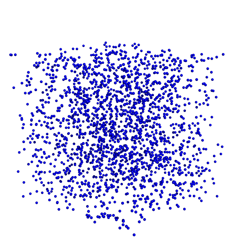
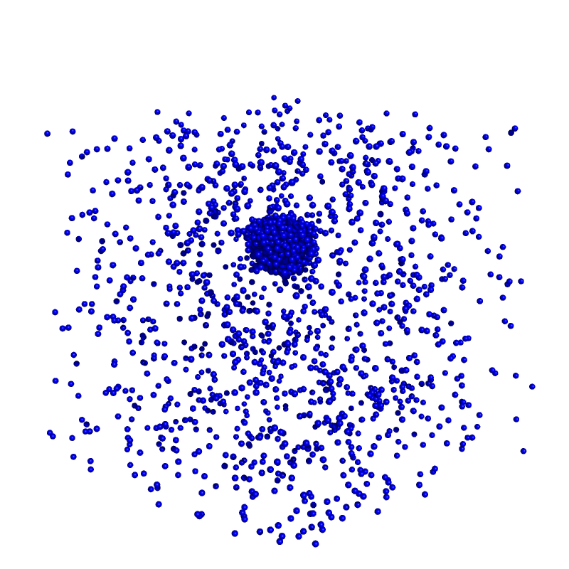
Figure 1: Illustration of a three-dimensional Lennard-Jones gas (left) and a droplet in equilibrium with surrounding vapor (right). Shown is a system with $N=2048$ particles at density $\rho=10^{-2}$ in a box with periodic boundary conditions.

A crucial aspect is the selection of Monte Carlo updates. While in Ref. [13] we restricted ourselves to local particles shifts, we added here particle “jumps” with a larger update range. The update range for a particle shift was set to $r=0.3$ and for a particle jump to $r=L/2$. A new position is then selected with equal probability from a sphere of size $r$ around the old position. This simple non-local update significantly enhanced the sampling of the gaseous phase and increased the performance of the simulation drastically. Instead of $512$ we are now able to sample up to $2048$ particles.

3 Theory

Here we only want to briefly recapture the results of many previous works [2, 3, 4, 5, 13]. For a supersaturated gas, it was shown that the probability of intermediate-sized droplets vanishes [3, 4], which leaves us with the scenario of a homogeneous gas phase on the one side and a droplet in equilibrium with surrounding vapor on the other side, see Fig. 1. At a fixed temperature, the droplet formation may be achieved by adding more particle excess to the already supersaturated gas. For both sides it is possible to formulate a contribution to the free-energy in terms of fluctuations (entropy of the gaseous phase) and surface tension (energy of the droplet). Importantly, the finite-size dependence could be rewritten in terms of the fraction of particle excess in the droplet as a function of a dimensionless density. This in turn allowed us to expand the results around the infinite-size transition temperature $T_{0}$ to yield the leading finite-size scaling behavior of the condensation temperature $T_{c}$ at fixed density [13]. Similarly, we showed that an expansion of the free-energy difference at the condensation transition yields an estimate of the leading-order finite-size scaling of the transition rounding $\Delta T$, i.e., the width of the transition. For details we refer to the prior literature and give here only the three-dimensional results to leading order:

$$T_{c}-T_{0} \propto N^{-1/4},$$ (3)

$$\Delta T \propto N^{-3/4}.$$ (4)

A crucial observation is now that the size $R$ of the droplet at the condensation transition itself scales non-trivially with system size, namely in three dimensions $R\propto N^{1/4}$. Thus, the leading-order scaling may be identified in terms of powers of the linear extension of the droplet itself, $\propto R^{-1}$ respectively $\propto R^{-3}$. This is consistent with the interpretation that the droplet size at transition is the relevant system size. Then, a virtual subsystem around the droplet would lead to a transition between a homogeneous liquid (droplet) phase to a homogeneous gas phase with open boundary conditions. The competition between finite-size contributions from volume ($\propto R^{3}$) and surface ($\propto R^{2}$) would in this case give rise to an intuitive finite-size correction of the order $R^{-1}$ [21, 22, 23, 13, 14].

4 Results

Due to the non-local Monte Carlo update, we are now able to extend our previous results [13] for the three-dimensional Lennard-Jones system to $N=2048$ particles with improved statistics. The temperature scale is fixed by setting $k_{\rm B}=1$. The finite-size transition temperature $T_{c}$ is obtained as the location of the largest peak in the specific heat $C_{V}=k_{\rm B}\beta^{2}\left(\langle E^{2}\rangle-\langle E\rangle^{2}\right)/N$ and plotted in Fig. 2 (left) versus the expected scaling behavior Eq. (3). Overall, the data qualitatively shows a linear behavior as predicted. A leading-order fit for $N\geq 1024$ yields $T_{0}=0.7032(3)$ with goodness-of-fit parameter $Q\approx 0.1$, shown in the figure as dashed black line. Including additional higher-order corrections, i.e., $T_{c}=T_{0}+aN^{-1/4}+bN^{-2/4}$, yields $T_{0}=0.6979(2)$ for $N\geq 64$ with $Q\approx 0.1$. Both estimates differ from our previous results outside the error bars, which is expected because the fit error underestimates systematic uncertainties. This is partially due to the fact that we are not yet fully in the asymptotic scaling regime, which we will discuss below. The general trend of the results is compatible with our previous conclusion, where we already noted that the available three-dimensional Lennard-Jones system sizes were too small for clear results. However, it is worth noting that the current estimates are closer to each other, implying an infinite-size limit of the transition temperature around $T_{0}\approx 0.70$.

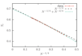
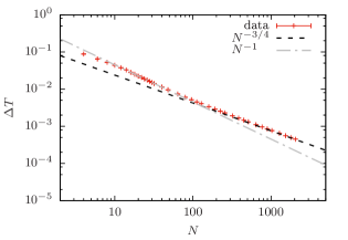
Figure 2: Finite-size scaling of the transition temperature (left) and rounding (right) as the maximum location and the half width of the specific-heat peak, respectively. Error bars are included but smaller than the symbol size.

The distance from the asymptotic scaling regime is best visible in the rounding of the transition. This is here obtained from the half width of the specific-heat peak, i.e., the width for which $C_{V}(T)>C_{V}^{\rm max}/2$, shown in Fig. 2 (right). Since the width vanishes in the thermodynamic limit, a double-logarithmic plot reveals the power-law scaling Eq. (4) as a straight line, here dashed black. As previously noticed [13], an intermediate scaling regime $\propto N^{-1}$ is clearly visible and marked with a dashed-dotted gray line. This is consistent with the droplet as relevant system size as in this regime still a large fraction of particles contribute to the transition droplet. However, for $N\geq 500$ it appears that the asymptotic scaling behavior slowly manifests itself and leading-order estimates become more reliable.

This can be tested by performing a direct fit of the power-law ansatz $\Delta T\propto N^{-\alpha}$, shown in Fig. 3 for variable lower bound $N_{\rm min}$. Only for $N_{\rm min}\geq 640$ the fit yields plausible goodness-of-fit values $Q>0.1$. Still, the distance to the predicted asymptotic scaling regime is noticeable. This is consistent with results obtained for the three-dimensional lattice gas where decent results were only obtained for $N_{\rm min}\approx 2000$ [13]. This emphasizes once more that care has to be taken with leading-order finite-size scaling away from the asymptotic scaling regime. While estimates of the thermodynamic limit become better with increasing system size, fit errors are difficult to judge because the underlying ansatz is not accurate enough. The same holds true for additional higher-order corrections. While the results are surely good estimates, the fit errors are a difficult measure, not capturing the uncertainty that comes from an incomplete fit model [24].

5 Conclusions

We have extended our previous results [13] for the three-dimensional Lennard-Jones system to larger system sizes. This allows for more consistent estimates of the thermodynamic limit when considering leading-order and higher-order fits. Still, the current Lennard-Jones system with up to $2048$ particles at density $\rho=10^{-2}$ is quite far away from the asymptotic scaling limit. We notice that the rounding of the transition is a good indicator to visualize this distance from the asymptotic scaling regime. Here, also the emerging intermediate scaling regime is best noticeable.

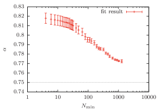
Figure 3: Results of direct fits of the ansatz $\Delta T\propto N^{-\alpha}$ to the data in Fig. 2 (right) with variable lower bound $N_{\rm min}$. The dotted line shows the predicted asymptotic scaling exponent.

References

References

- [1] Binder K and Kalos M H 1980 J. Stat. Phys. 22 363
- [2] Neuhaus T and Hager J 2003 J. Stat. Phys. 113 47
- [3] Biskup M, Chayes L and Kotecký R 2002 Europhys. Lett. 60 32
- [4] Biskup M, Chayes L and Kotecký R 2003 Commun. Math. Phys. 242 137
- [5] Binder K 2003 Physica A 319 99
- [6] Nußbaumer A, Bittner E, Neuhaus T and Janke W 2006 Europhys. Lett. 75 716
- [7] Nußbaumer A, Bittner E and Janke W 2008 Phys. Rev. E 77 041109
- [8] Zierenberg J, Wiedenmann M and Janke W 2014 J. Phys.: Conf. Ser. 510 012017
- [9] MacDowell L G, Virnau P, Müller M and Binder K 2004 J. Chem. Phys. 120 5293
- [10] MacDowell L G, Shen V K and Errington J R 2006 J. Chem. Phys. 125 034705
- [11] Schrader M, Virnau P and Binder K 2009 Phys. Rev. E 79 061104
- [12] Martinos S, Malakis A and Hadjiagapiou I 2007 Physica A 384 368
- [13] Zierenberg J and Janke W 2015 Phys. Rev. E 92 012134
- [14] Zierenberg J, Mueller M, Schierz P, Marenz M and Janke W 2014 J. Chem. Phys. 141 114908
- [15] Berg B A and Neuhaus T 1991 Phys. Lett. B 267 249
- [16] Berg B A and Neuhaus T 1992 Phys. Rev. Lett. 68 9
- [17] Janke W 1992 Int. J. Mod. Phys. C 3 1137
- [18] Janke W 1998 Physica A 254 164
- [19] Zierenberg J, Marenz M and Janke W 2013 Comput. Phys. Commun. 184 1155
- [20] Zierenberg J, Marenz M and Janke W 2014 Physics Procedia 53 55
- [21] Privman V and Rudnick J 1990 J. Stat. Phys. 60 551
- [22] Borgs C and Kotecký R 1995 J. Stat. Phys. 79 43
- [23] Borgs C, Kotecký R and Medved I 2002 J. Stat. Phys. 109 67
- [24] Young P 2015 Everything You Wanted to Know About Data Analysis and Fitting but Were Afraid to Ask, SpringerBriefs in Physics (Springer International Publishing) [arXiv:1210.3781 (2012)]