Nonradial stability of marginal stable circular orbits in stationary axisymmetric spacetimes

Abstract

We study linear nonradial perturbations and stability of a marginal stable circular orbit (MSCO) such as the innermost stable circular orbit (ISCO) of a test particle in stationary axisymmetric spacetimes which possess a reflection symmetry with respect to the equatorial plane. A zenithal stability criterion is obtained in terms of the metric components, the specific energy and angular momentum of a test particle. The proposed approach is applied to Kerr solution and Majumdar-Papapetrou solution to Einstein equation. Moreover, we reexamine MSCOs for a modified metric of a rapidly spinning black hole that has been recently proposed by Johannsen and Psaltis [PRD, 83, 124015 (2011)]. We show that, for the Johannsen and Psaltis’s model, circular orbits that are stable against radial perturbations for some parameter region become unstable against zenithal perturbations. This suggests that the last circular orbit for this model may be larger than the ISCO.

I Introduction

GW150914 event that has been eventually discovered by the two aLIGO detectors fits well with a binary black hole inspiraling and merger model GW150914PRL ; GW150914ApJL . It is likely that there exists the innermost stable circular orbit (ISCO) for the binary black hole. In gravitational wave astronomy, ISCOs are thought to be the last circular orbit corresponding to the transition point from the inspiraling phase to the merging one. In the post-Newtonian approximation, the dynamical stability of circular orbits of a two-body system has been studied. See Ref. Blanchet for a comprehensive review on the post-Newtonian approximation: The 1PN term gives exactly the ISCO radius for the Schwarzschild case, but for any mass ratio. The finite mass corrections on the ISCO radius appear at the 2PN order. At the 3PN order, all the circular orbits are stable when the mass ratio is larger than some critical value $\nu_{C}\sim 0.183$ (See e.g. Section 8.2 in Blanchet ). However, there is an ISCO at the 3PN order, when the mass ratio is smaller than the critical value. Moreover, at the 4PN (and higher PN) orders, finite mass corrections on the ISCO radius may appear Blanchet-priv . In black hole perturbation theory, Isoyama et al. have discussed the ISCO of a small particle around a Kerr black hole and have computed the linear-order correction in the mass ratio Isoyama .

In high energy astrophysics, furthermore, ISCOs are related to the inner edge of an accretion disk around a black hole Abramowicz . Therefore, the ISCOs would help us to test the nonlinear spacetime geometry that is beyond the solar-system experiments. It is important to study the nature of the ISCOs around black holes with electric charges and/or scalar fields no-hair and black holes in modified gravity theories modified .

Ono et al. have recently reexamined, in terms of Sturm’s theorem Algebra , marginal stable circular orbits (MSCOs) of a test particle in spherically symmetric and static spacetimes Ono . The wording “marginal stable circular orbits” is used, because the wording “marginally stable” has a different meaning in the theory of dynamical systems. It is interesting to extend such previous works no-hair ; modified ; Ono to stationary and axisymmetric cases, because astrophysical black holes are likely to spin GW150914PRL ; GW150914ApJL . Indeed, Stute and Camenzind have found an equation for the MSCO radius Stute , where the particle is assumed to move on the equatorial plane. However, their analysis is limited within the radial perturbation.

The main purpose of this paper is to extend such a MSCO study to stationary and axisymmetric spacetimes, and furthermore, by taking account of not only the radial perturbation but also the nonradial perturbation. In particular, a zenithal stability criterion for a test particle in a MSCO is derived in terms of the metric components, the specific energy and angular momentum of a test particle. We shall apply the proposed approach to three models: Kerr solution, Majumdar-Papapetrou solution to the Einstein equation MP1 ; MP2 , and Johannsen and Psaltis’s model of a rapidly spinning black hole in modified gravity JP .

Throughout this paper, we use the unit of $G=c=1$.

II Marginal stable circular orbit

We consider a stationary axisymmetric spacetime. The line element for this spacetime is Lewis ; LR ; Papapetrou

$$ds^{2}= g_{\mu\nu}dx^{\mu}dx^{\nu}$$

$$= -A(y^{p},y^{q})dt^{2}-2H(y^{p},y^{q})dtd\phi$$

$$+F(y^{p},y^{q})(\gamma_{pq}dy^{p}dy^{q})+D(y^{p},y^{q})d\phi^{2},$$ (1)

where $\mu,\nu$ run from $0$ to $3$, $p,q$ take $1$ and $2$, $t$ and $\phi$ coordinates are associated with the Killing vectors, and $\gamma_{pq}$ is a two-dimensional symmetric tensor. It is more convenient to reexpress this metric into a form in which $\gamma_{pq}$ is diagonalized. The present paper prefers the polar coordinates rather than the cylindrical ones, because we consider the Kerr metric and its modified metric by Johannsen and Psaltis JP in the polar coordinates. Then, Eq. (1) becomes Metric

$$ds^{2}= -A(r,\theta)dt^{2}-2H(r,\theta)dtd\phi$$

$$+B(r,\theta)dr^{2}+C(r,\theta)d\theta^{2}+D(r,\theta)d\phi^{2}.$$ (2)

The present paper focuses on a test particle outside the horizon. Then, $\det{(g_{\mu\nu})}<0$. This leads to $B(r,\theta)\neq 0$, $C(r,\theta)\neq 0$ and $A(r,\theta)D(r,\theta)+H^{2}(r,\theta)\neq 0$. We assume also a local reflection symmetry with respect to the equatorial plane as Reflection

$$\left.\frac{\partial g_{\mu\nu}}{\partial\theta}\right|_{\theta=\pi/2}=0,$$ (3)

where we choose $\theta=\pi/2$ as the equatorial plane.

We denote the contravariant metric tensor as

$${g}^{\mu\nu} =\left(\begin{array}[]{cccc}-\frac{D}{AD+H^{2}}&0&0&-\frac{H}{AD+H^{2}}\\ 0&\frac{1}{B}&0&0\\ 0&0&\frac{1}{C}&0\\ -\frac{H}{AD+H^{2}}&0&0&\frac{A}{AD+H^{2}}\end{array}\right)$$ (8)

$$\equiv\left(\begin{array}[]{cccc}-\tilde{A}&0&0&-\tilde{H}\\ 0&\tilde{B}&0&0\\ 0&0&\tilde{C}&0\\ -\tilde{H}&0&0&\tilde{D}\end{array}\right)　.$$ (13)

Let us define the Lagrangian of the test particle as

$${\cal L}=-A\dot{t}^{2}-2H\dot{t}\dot{\phi}+B\dot{r}^{2}+C\dot{\theta}^{2}+D\dot{\phi}^{2},$$ (14)

where the dot denotes the derivative with respect to the proper time. There are two constants of motion for the test body, because the spacetime is stationary and axisymmetric.

$$\varepsilon =-A\dot{t}-H\dot{\phi},$$ (15)

$$\ell =-H\dot{t}+D\dot{\phi},$$ (16)

where $\varepsilon$ and $\ell$ are corresponding to the specific energy and the specific angular momentum, respectively.

Let us examine linear perturbations around the equatorial marginal circular orbit (denoted as $r=r_{c}$), in which the perturbed position is denoted as $r=r_{c}+\delta r$ and $\theta=\pi/2+\delta\theta$. We consider the geodesic equation at the perturbed position and examine the linear parts in $\delta r$ and $\delta\theta$. Straightforward calculations show that $\delta r$-parts and $\delta\theta$-ones are decoupled with each other in the geodesic equation.

First, we consider the $r$-component of the geodesic equation in the Taylor series approximation such as $A(r,\theta)=A(r_{c},\pi/2)+\delta r\times\partial A(r,\pi/2)/\partial r|_{r=r_{C}}+\cdots$, where we use the local reflection symmetry of the metric with respect to the equatorial plane, and $\dot{t}$ and $\dot{\phi}$ are rewritten in terms of $\varepsilon$ and $\ell$ by using Eqs. (15) and (16). Hence, we obtain

$$\left.\frac{\partial\tilde{A}}{\partial r}\right|_{c}\varepsilon^{2}+2\left.\frac{\partial\tilde{H}}{\partial r}\right|_{c}\varepsilon l-\left.\frac{\partial\tilde{D}}{\partial r}\right|_{c}l^{2}=0,$$ (17)

at the zeroth order (namely, $r=r_{C}$ and $\theta=\pi/2$) and

$$\left.\frac{\partial^{2}\tilde{A}}{\partial r^{2}}\right|_{c}\varepsilon^{2}+2\left.\frac{\partial^{2}\tilde{H}}{\partial r^{2}}\right|_{c}\varepsilon l-\left.\frac{\partial^{2}\tilde{D}}{\partial r^{2}}\right|_{c}l^{2}=0,$$ (18)

at the linear order, where $|_{C}$ denotes the position at $r=r_{C}$ and $\theta=\pi/2$.

Next, the $\theta$-component of the geodesic equation gives us a stable condition to the zenithal perturbation as

$$\left.\frac{\partial^{2}\tilde{A}}{\partial\theta^{2}}\right|_{c}\varepsilon^{2}+2\left.\frac{\partial^{2}\tilde{H}}{\partial\theta^{2}}\right|_{c}\varepsilon l-\left.\frac{\partial^{2}\tilde{D}}{\partial\theta^{2}}\right|_{c}l^{2}<0,$$ (19)

which plays a crucial role in this paper. The inequality sign changes if the orbit is unstable against the zenithal perturbation. Henceforth, we omit the notation $|_{C}$ for brevity. See e.g. page 362 in Chandrasekhar (1998) for a description of the $\theta$-motion in a well-known black hole solution such as Kerr solution Chandrasekhar . Note that a zenithal stability criterion by Eq. (19) is new.

By combining Eqs. (17) and (18) in the similar manner to the spherically symmetric case (See e.g. Ono ; BJS ; RZ ), we obtain

$$\left[\frac{\partial\tilde{D}}{\partial r}\frac{\partial^{2}\tilde{A}}{\partial r^{2}}-\frac{\partial\tilde{A}}{\partial r}\frac{\partial^{2}\tilde{D}}{\partial r^{2}}\right]^{2}$$

$$-4\left[\frac{\partial\tilde{A}}{\partial r}\frac{\partial^{2}\tilde{H}}{\partial r^{2}}-\frac{\partial\tilde{H}}{\partial r}\frac{\partial^{2}\tilde{A}}{\partial r^{2}}\right]\left[\frac{\partial\tilde{D}}{\partial r}\frac{\partial^{2}\tilde{H}}{\partial r^{2}}-\frac{\partial\tilde{H}}{\partial r}\frac{\partial^{2}\tilde{D}}{\partial r^{2}}\right]=0.$$ (20)

After straightforward calculations, one can show that this agrees with the Stute and Camenzind’s equation for the MSCO radius Stute . Beheshti and Gasperin Beheshti rediscovered in a mathematical way the Stute and Camenzind’s equation, which is, to be precise, a necessary condition for the existence of MSCOs. Note that Eq. (20) is shorter. See Eq. (40) in Stute . This is only because we use the contravariant metric components. We call Eq. (20) a MSCO equation for brevity. See Appendix for derivations of Eq. (20).

Before closing this section, let us write down the expression for the squared specific energy and the squared specific angular momentum as

$$\varepsilon^{2}=$$

$$\frac{\tilde{A}\left\{\frac{-\frac{\partial\tilde{H}}{\partial r}\pm\sqrt{(\frac{\partial\tilde{H}}{\partial r})^{2}+\frac{\partial\tilde{A}}{\partial r}\frac{\partial\tilde{D}}{\partial r}}}{\frac{\partial\tilde{A}}{\partial r}}\right\}^{2}}{\left[\frac{\tilde{A}}{\frac{\partial\tilde{A}}{\partial r}}\left\{-\frac{\partial\tilde{H}}{\partial r}\pm\sqrt{\left(\frac{\partial\tilde{H}}{\partial r}\right)^{2}+\frac{\partial\tilde{A}}{\partial r}\frac{\partial\tilde{D}}{\partial r}}\right\}+\tilde{H}\right]^{2}-\tilde{H}^{2}-\tilde{A}\tilde{D}},$$ (21)

$$\ell^{2}=$$

$$\frac{\tilde{A}}{\left[\frac{\tilde{A}}{\frac{\partial\tilde{A}}{\partial r}}\left\{-\frac{\partial\tilde{H}}{\partial r}\pm\sqrt{\left(\frac{\partial\tilde{H}}{\partial r}\right)^{2}+\frac{\partial\tilde{A}}{\partial r}\frac{\partial\tilde{D}}{\partial r}}\right\}+\tilde{H}\right]^{2}-\tilde{H}^{2}-\tilde{A}\tilde{D}}.$$ (22)

Note that Eqs. (21) and (22) hold for not only MSCOs but also general circular orbits.

III Applications to stationary axisymmetric models

III.1 Kerr solution

Let us consider the Kerr metric

$$ds^{2}= -\left(1-\frac{2Mr}{\Sigma}\right)dt^{2}-\frac{4aMr\sin^{2}\theta}{\Sigma}dtd\phi$$

$$+\frac{\Sigma}{\Delta}dr^{2}+\Sigma d\theta^{2}$$

$$+\left(r^{2}+a^{2}+\frac{2a^{2}Mr\sin^{2}\theta}{\Sigma}\right)\sin^{2}\theta d\phi^{2},$$ (23)

where $\Sigma=r^{2}+a^{2}\cos^{2}\theta$ and $\Delta=r^{2}-2Mr+a^{2}$. Then, Eq. (20) becomes

$$\overline{r}^{4}-12\overline{r}^{3}+(-6\overline{a}^{2}+36)\overline{r}^{2}-28\overline{a}^{2}\overline{r}+9\overline{a}^{4}=0,$$ (24)

where $r$ and $a$ are normalized as $\bar{r}\equiv r/M$ and $\bar{a}\equiv a/M$. This quartic equation is solved to recover the known result. See Eq. (2.21) in BPT . The zenithal stable condition by Eq. (19) is satisfied. Therefore, the same radius holds against the zenithal perturbation. See Figure 1 for the ISCO location.

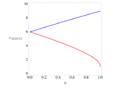
Figure 1: MSCOs around a Kerr black hole. The vertical axis denotes the ISCO radius in the unit of $M$. The horizontal axis denotes the spin parameter $a$. The upper curve (blue in color) corresponds to the retrograde case and the lower curve (red in color) corresponds to the prograde one.

III.2 Majumdar-Papapetrou solution

Next, we consider the Majumdar-Papapetrou solution to Einstein equation MP1 ; MP2 . This solution expresses a superposition of extreme Reissner-Nordström solutions. The spacetime metric is

$$ds^{2} =-\Omega^{-2}dt^{2}+\Omega^{2}(dx^{2}+dy^{2}+dz^{2}),$$ (25)

where we define

$$\Omega= 1+\sum_{i}\frac{m_{i}}{r_{i}},$$

$$r_{i}= \sqrt{(x-x_{i})^{2}+(y-y_{i})^{2}+(z-z_{i})^{2}}.$$ (26)

We focus on a case of two equal-mass black holes, where they are located at $(0,0,L)$ and $(0,0,-L)$ along the $z$ axis. By using the polar coordinates, Eq. (20) for this equal-mass case becomes

$$r^{6}+r^{4}\left(6L^{2}-6M\sqrt{L^{2}+r^{2}}\right)$$

$$+r^{2}\left(9L^{4}+10L^{2}M\sqrt{L^{2}+r^{2}}\right)$$

$$+16L^{4}M\sqrt{L^{2}+r^{2}}+4L^{4}(L^{2}+4M^{2})=0,$$ (27)

where $M$ is the black hole mass. By introducing $s\equiv(r^{2}+L^{2})^{1/2}$, this long equation is reduced to

$$s^{6}-6Ms^{5}+3L^{2}s^{4}+22L^{2}Ms^{3}+16L^{4}M^{2}=0.$$ (28)

Exact solutions for a sixth-degree equation are not known. Therefore, we have to solve numerically Eq. (28).

The gravitational pull by the two black holes along the $z$ axis is unlikely to stabilize the particle position. Some of the equatorial circular orbits are indeed unstable against nonradial perturbations. See Figure 2.

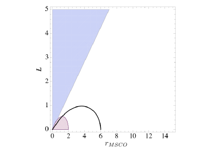
Figure 2: MSCOs for the Majumdar-Papapetrou solution, where we focus on two equal-mass black hole cases. The vertical axis denotes $L$ in the unit of $M$. The horizontal axis denotes the MSCO radius. The solid curve (black in color) is the MSCOs. The orbit is radially unstable in the inner area surrounded by the solid curve, while it is radially stable in the outer region. The lightly shaded region (blue in color) denotes the forbidden region where the orbit is unstable against the zenithal perturbation. In the dark shaded region (magenta in color), the orbit is unstable to the zenithal perturbation and $\varepsilon^{2}<0$ or $\ell^{2}<0$. Two MSCOs are possible, if $L$ is between $\sim 0.6$ and $\sim 1.0$.

Figure 3: MSCOs in Johannsen and Psaltis’s modified model of a rapidly spinning black hole. The vertical axis denotes the MSCO radius in the unit of $M$. The horizontal axis denotes the black hole spin parameter. The solid curve (black in color) denotes the ISCOs. The upper part of the solid curve ($r$ is larger than $\sim 5.6$) corresponds to the retrograde case and the lower part ($r$ is smaller than $\sim 5.6$) corresponds to the prograde one. The lightly shaded region (blue in color) denotes the forbidden region where the orbit is unstable against the zenithal perturbation. In the dark shaded region (magenta in color), the orbit is unstable against the zenithal perturbation and $\varepsilon^{2}<0$ or $\ell^{2}<0$. The other solid curve (red in color) denotes the horizon. There exist outer and inner horizons, when $a$ is smaller than $\sim 0.7m$. They merge at $a\sim 0.7m$.

III.3 Johannsen and Psaltis’s model for a modified Kerr metric

Finally, we examine Johannsen and Psaltis’s modified Kerr metric as JP

$$ds^{2}= -[1+h(r,\theta)]\left(1-\frac{2Mr}{\Sigma}\right)dt^{2}$$

$$-\frac{4aMr\sin^{2}\theta}{\Sigma}\times[1+h(r,\theta)]dtd\phi$$

$$+\frac{\Sigma[1+h(r,\theta)]}{\Delta+a^{2}\sin^{2}\theta h(r,\theta)}dr^{2}+\Sigma d\theta^{2}$$

$$+\left[\sin^{2}\theta\left(r^{2}+a^{2}+\frac{2a^{2}Mr\sin^{2}\theta}{\Sigma}\right)\right.$$

$$~{}~{}~{}~{}~{}\left.+h(r,\theta)\frac{a^{2}(\Sigma+2Mr)\sin^{4}\theta}{\Sigma}\right]d\phi^{2},$$ (29)

where we define

$$h(r,\theta)\equiv\epsilon_{3}\frac{M^{3}r}{\Sigma^{2}}.$$ (30)

The new parameter $\epsilon_{3}$ is not constrained by observations so far JP .

For the model proposed by Johannsen and Psaltis, Eq. (20) becomes explicitly

$$4r^{22}\Big{[}9a^{4}+(6M-r)^{2}r^{2}-2a^{2}r(14M+3r)\Big{]}$$

$$+4M^{2}r^{19}\epsilon_{3}$$

$$~{}~{}\times\Big{[}3a^{4}(4M-15r)$$

$$~{}~{}~{}~{}~{}~{}+(6M-r)\left(36M^{2}-4Mr-3r^{2}\right)r^{2}$$

$$~{}~{}~{}~{}~{}~{}+2a^{2}r\left(2M^{2}-69Mr+3r^{2}\right)\Big{]}$$

$$+M^{4}r^{15}\epsilon_{3}^{2}$$

$$~{}~{}\times\Big{[}-360a^{6}M+r^{3}\left(36M^{2}-4Mr-3r^{2}\right)^{2}$$

$$~{}~{}~{}~{}~{}~{}+4M(6M-r)r^{3}\left(96M^{2}-74Mr+15r^{2}\right)$$

$$~{}~{}~{}~{}~{}~{}+3a^{4}r\left(224M^{2}-696Mr+75r^{2}\right)$$

$$~{}~{}~{}~{}~{}~{}+2a^{2}r^{2}\left(880M^{3}-1344M^{2}r+102Mr^{2}+45r^{3}\right)\Big{]}$$

$$+2M^{7}r^{12}\epsilon_{3}^{3}$$

$$~{}~{}\times\Big{[}-1116a^{6}M+48a^{4}r\left(35M^{2}-84Mr+15r^{2}\right)$$

$$~{}~{}~{}~{}~{}~{}+r^{3}\left(36M^{2}-4Mr-3r^{2}\right)\left(96M^{2}-74Mr+15r^{2}\right)$$

$$~{}~{}~{}~{}~{}~{}+a^{2}r^{2}\left(5056M^{3}-6384M^{2}r+1854Mr^{2}-81r^{3}\right)\Big{]}$$

$$+M^{10}r^{9}\epsilon_{3}^{4}$$

$$~{}~{}\times\Big{[}-5976a^{6}M+r^{3}\left(96M^{2}-74Mr+15r^{2}\right)^{2}$$

$$~{}~{}~{}~{}~{}~{}+24a^{4}r\left(398M^{2}-723Mr+171r^{2}\right)$$

$$~{}~{}~{}~{}~{}~{}+8a^{2}r^{2}\left(2432M^{3}-3174M^{2}r+1227Mr^{2}-135r^{3}\right)\Big{]}$$

$$+8a^{2}M^{13}r^{6}\epsilon_{3}^{5}$$

$$~{}~{}\times\Big{[}-1017a^{4}M$$

$$~{}~{}~{}~{}~{}~{}+6a^{2}r\left(284M^{2}-435Mr+120r^{2}\right)$$

$$~{}~{}~{}~{}~{}~{}+r^{2}\left(2344M^{3}-3306M^{2}r+1515Mr^{2}-225r^{3}\right)\Big{]}$$

$$+24a^{4}M^{16}r^{3}\epsilon_{3}^{6}$$

$$~{}~{}\times\Big{[}-228a^{2}M+r\left(404M^{2}-525Mr+150r^{2}\right)\Big{]}$$

$$-1440a^{6}M^{20}\epsilon_{3}^{7}=0.$$ (31)

See Figure 3 for a numerical result. Here, we choose $\epsilon_{3}=2$, such that the effects by the modification in the figure can be seen by eye. Circular orbits that are stable to radial perturbations for some parameter region are unstable to nonradial perturbations. This thing has not been known so far, because Johannsen and Psaltis JP consider only the radial perturbations.

IV Conclusion

We performed a linear stability analysis to nonradial perturbations of a marginal stable circular orbit of a test particle in stationary axisymmetric spacetimes. A zenithal stability criterion was obtained as Eq. (19). The proposed approach was applied to Kerr solution and Majumdar-Papapetrou solution to Einstein equation. Moreover, we suggested that, for the Johannsen and Psaltis’s model, circular orbits that are stable to radial perturbations for some parameter region become unstable against zenithal perturbations. This implies that, at least for the Johannsen and Psaltis’s model, the last circular orbit might be larger than the ISCO, because the ISCO (in the usual sense) often refers to the smallest circular orbit that is stable against the radial perturbation. Blanchet ; Isoyama ; Ono ; Stute ; BJS ; RZ ; Beheshti ; Text It is left as a future work to study a more general case.

Appendix A Derivations of Eq. (20)

In this section, we discuss the derivation of Eq. (20), where $\varepsilon\neq 0$ and $\ell\neq 0$. A method of deriving Eq. (20) is using not only Eqs. (17) and (18) but also the equation defining the proper time along the particle orbit that is expressed as $-1=A\dot{t}^{2}+\cdots$. By using Eqs. (15) and (16), one can show that the three equations are linear in $\varepsilon^{2}$, $\ell^{2}$ and $\varepsilon\ell$. They are easily solved for $\varepsilon^{2}$, $\ell^{2}$ and $\varepsilon\ell$. A consistency condition as $(\varepsilon\ell)^{2}=\varepsilon^{2}\times\ell^{2}$ gives Eq. (20).

It is interesting to mention another but shorter derivation. Let $p$ and $q$ denote the left hand sides of Eqs. (17) and (18), respectively. They are polynomials in $\varepsilon$ and $\ell$ and therefore they are rearranged as

$$p\frac{\partial^{2}\tilde{D}}{\partial r^{2}}= q\frac{\partial\tilde{D}}{\partial r}+\left(\frac{\partial\tilde{A}}{\partial r}\frac{\partial^{2}\tilde{D}}{\partial r^{2}}-\frac{\partial\tilde{D}}{\partial r}\frac{\partial^{2}\tilde{A}}{\partial r^{2}}\right)\varepsilon^{2}$$

$$+2\left(\frac{\partial\tilde{H}}{\partial r}\frac{\partial^{2}\tilde{D}}{\partial r^{2}}-\frac{\partial\tilde{D}}{\partial r}\frac{\partial^{2}\tilde{H}}{\partial r^{2}}\right)\varepsilon\ell,$$ (32)

$$p\frac{\partial^{2}\tilde{A}}{\partial r^{2}}= q\frac{\partial\tilde{A}}{\partial r}+2\left(\frac{\partial\tilde{H}}{\partial r}\frac{\partial^{2}\tilde{A}}{\partial r^{2}}-\frac{\partial\tilde{A}}{\partial r}\frac{\partial^{2}\tilde{H}}{\partial r^{2}}\right)\varepsilon\ell$$

$$+\left(\frac{\partial\tilde{A}}{\partial r}\frac{\partial^{2}\tilde{D}}{\partial r^{2}}-\frac{\partial\tilde{D}}{\partial r}\frac{\partial^{2}\tilde{A}}{\partial r^{2}}\right)\ell^{2},$$ (33)

Therefore, Eqs. (17) and (18) are equivalent to

$$\left(\begin{array}[]{cc}\frac{\partial\tilde{A}}{\partial r}\frac{\partial^{2}\tilde{D}}{\partial r^{2}}-\frac{\partial\tilde{D}}{\partial r}\frac{\partial^{2}\tilde{A}}{\partial r^{2}}&2\frac{\partial\tilde{H}}{\partial r}\frac{\partial^{2}\tilde{D}}{\partial r^{2}}-2\frac{\partial\tilde{D}}{\partial r}\frac{\partial^{2}\tilde{H}}{\partial r^{2}}\\ 2\frac{\partial\tilde{H}}{\partial r}\frac{\partial^{2}\tilde{A}}{\partial r^{2}}-2\frac{\partial\tilde{A}}{\partial r}\frac{\partial^{2}\tilde{H}}{\partial r^{2}}&\frac{\partial\tilde{A}}{\partial r}\frac{\partial^{2}\tilde{D}}{\partial r^{2}}-\frac{\partial\tilde{D}}{\partial r}\frac{\partial^{2}\tilde{A}}{\partial r^{2}}\end{array}\right)\left(\begin{array}[]{c}\varepsilon\\ l\end{array}\right)$$ (38)

$$=\left(\begin{array}[]{c}0\\ 0\end{array}\right).$$ (41)

A necessary condition for avoiding simultaneously $\varepsilon=0$ and $\ell=0$ is that the determinant of the matrix in the left hand side of Eq. (41) vanishes. Eq. (20) is thus derived.

References

• (1) B. P. Abbott., et al. Phys. Rev. Lett. 116, 061102 (2016).
• (2) B. P. Abbott., et al. Astrophys. J. Lett. 818, L22 (2016).
• (3) L. Blanchet, Living Rev. Relativ. 17, 2 (2014).
• (4) L. Blanchet, private communications.
• (5) S. Isoyama, L. Barack, S. R. Dolan, A. Le Tiec, H. Nakano, A. G. Shah, T. Tanaka, and N. Warburton, Phys. Rev. Lett. 113, 161101 (2014).
• (6) B. P. Abbott., et al. Phys. Rev. Lett. 116, 241103 (2016).
• (7) M. A. Abramowicz, M. Jaroszynski, S. Kato, J. P. Lasota, A. Rozanska, and A. Sadowski, Astron. Astrophys. 521, A15 (2010).
• (8) C. Bambi and K. Freese, Phys. Rev. D 79, 043002 (2009); T. Johannsen and D. Psaltis, Astrophys. J. 716, 187 (2010); 718, 446 (2010); A. E. Broderick, T. Johannsen, A. Loeb, and D. Psaltis, Astrophys. J. 784, 7 (2014).
• (9) P. Kanti, N. E. Mavromatos, J. Rizos, K. Tamvakis, and E. Winstanley, Phys. Rev. D 54, 5049 (1996); 57, 6255 (1998); N. Yunes and F. Pretorius, Phys. Rev. D 79, 084043 (2009); E. Barausse, T. Jacobson, and T. P. Sotiriou, Phys. Rev. D 83, 124043 (2011); R. A. Konoplya and A. Zhidenko, Rev. Mod. Phys. 83, 793 (2011); K. Yagi, N. Yunes, and T. Tanaka, Phys. Rev. D 86, 044037 (2012).
• (10) B. L. van der Waerden, Algebra I (Springer, 1966)
• (11) T. Ono, T. Suzuki, N. Fushimi, K. Yamada, and H. Asada, Europhys. Lett. 111, 30008 (2015).
• (12) M. Stute and M. Camenzind, Mon. Not. R. Soc. 336, 831 (2002).
• (13) S. D. Majumdar, Phys. Rev. 72, 390 (1947).
• (14) A. Papapetrou, Proc. Roy. Irish Acad. 51, 191 (1947).
• (15) T. Johannsen and D. Psaltis, Phys. Rev. D 83, 124015 (2011).
• (16) T. Lewis, Proc. Roy. Soc. A, 136, 176 (1932).
• (17) H. Levy, and W. J. Robinson, Proc. Camb. Phil. Soc. 60, 279 (1963).
• (18) A. Papapetrou, Ann. Inst. H. Poincare A, 4, 83 (1966).
• (19) In this paper, we use the polar coordinates. In the cylindrical coordinates, the line element is known as the Weyl-Lewis-Papapetrou form Lewis ; LR ; Papapetrou .
• (20) Note that this local condition suffices for the discussion in the present paper, though it does not guarantee the global existence of the spacetime.
• (21) S. Chandrasekhar, The Mathematical Theory of Black Holes, (Oxford University Press, New York, 1998).
• (22) E. Barausse, T. Jacobson, and T. P. Sotiriou, Phys. Rev. D 83, 124043 (2011).
• (23) L. Rezzolla, and A. Zhidenko, Phys. Rev. D 90, 084009 (2014).
• (24) S. Beheshti, and E. Gasperin, ArXiv:1512.08707.
• (25) J. M. Bardeen, W. H. Press, and S. A. Teukolsky, Astrophys. J. 178, 347 (1972).
• (26) L. D. Landau and E. M. Lifshitz, The Classical Theory of Fields (Pergamon, New York, 1962); S. Weinberg, Gravitation and Cosmology, (Wiley, New York, 1972); C. W. Misner, K. S. Thorne, J. A. Wheeler, Gravitation, (Freeman, New York, 1973); R. M. Wald, General Relativity, (The University of Chicago Press, 1984).