Studies of Spuriously Shifting Resonances in Time-dependent Density Functional Theory

Abstract

Adiabatic approximations in time-dependent density functional theory (TDDFT) will in general yield unphysical time-dependent shifts in the resonance positions of a system driven far from its ground-state. This spurious time-dependence is explained in [J. I. Fuks, K. Luo, E. D. Sandoval and N. T. Maitra, Phys. Rev. Lett. 114, 183002 (2015)] in terms of the violation of an exact condition by the non-equilibrium exchange-correlation kernel of TDDFT. Here we give details on the derivation and discuss reformulations of the exact condition that apply in special cases. In its most general form, the condition states that when a system is left in an arbitrary state, the TDDFT resonance position for a given transition in the absence of time-dependent external fields and ionic motion, is independent of the state. Special cases include the invariance of TDDFT resonances computed with respect to any reference interacting stationary state of a fixed potential, and with respect to any choice of appropriate stationary Kohn-Sham reference state. We then present several case studies, including one that utilizes the adiabatically-exact approximation, that illustrate the conditions and the impact of their violation on the accuracy of the ensuing dynamics. In particular, charge-transfer across a long-range molecule is hampered, and we show how adjusting the frequency of a driving field to match the time-dependent shift in the charge-transfer resonance frequency, results in a larger charge transfer over time.

I Introduction

The art of making approximations in the ab initio quantum theory of many-body systems enables us to investigate realistic systems of various sizes, ranging from atoms to biological molecules with affordable computational resources. Accurate but efficient approximations are crucial to reproduce the experimental results, improve our understanding of the mechanisms in play and make both qualitative and quantitative predictions. Rapid progress in experimental spectroscopy has begun to unveil dynamics of the electronic degrees of freedom on the timescale of tens of attoseconds, which provides a touchstone for the assessment of ab initio electronic structure theoriesKrausz and Ivanov (2009); Goulielmakis et al. (2010); Neppl et al. (2015).

Based on Runge-Gross theorem, time-dependent density functional theory(TDDFT) is an in-principle exact and efficient theoryRunge and Gross (1984); Marques et al. (2012); Ullrich (2011), that, with functional approximations inherited from ground state density functional theory stands out prominently among all other methods. The interacting one-body density $n({\bf r},t)$ is obtained from the evolution of the Kohn-Sham (KS) system, a system of fictitious non-interacting particles. The KS particles evolve under a one-body potential $v_{\scriptscriptstyle\rm S}({\bf r},t)$, following $i\partial_{t}\varphi_{k}({\bf r},t)=(-\frac{\nabla^{2}}{2}+v_{s}({\bf r},t))\varphi_{k}({\bf r},t)$, such that the interacting density is reproduced from $n({\bf r},t)=\sum_{k}^{\mathrm{occ}}|\varphi_{k}({\bf r},t)|^{2}$. The theory is in principle exact but the KS potential $v_{s}({\bf r},t)$ contains an unknown contribution called exchange-correlation (xc) potential $v_{\scriptscriptstyle\rm XC}({\bf r},t)$, which in practice needs to be approximated. The latter is a functional of the density at all points in space and at all previous times as well as the initial interacting state $\Psi_{0},$ and initial KS state $\Phi_{0}$: $v_{\scriptscriptstyle\rm XC}[n;\Psi_{0},\Phi_{0}](t)$.

Most TDDFT calculations however are adiabatic, i.e. the instantaneous density is plugged into a ground state functional, $v_{\scriptscriptstyle\rm XC}^{\rm adia}[n;\Psi_{0},\Phi_{0}](t)=v_{\scriptscriptstyle\rm XC}^{\rm g.s.}[n(t)]$, neglecting all dependence on the history of the density and on the initial states $\Psi_{0}$ and $\Phi_{0}$. Adiabatic linear response TDDFT is extensively and successfully used to compute excitation energies of molecules and solidsMarques et al. (2012) , but TDDFT is not limited to linear response: the theorems state that the density response to any order in an external perturbation can be reproduced. It is a promising candidate for modeling non-equilibrium electron dynamics since it can capture the correlation effects with a relatively cheap computational cost. Although the performance of available functionals for non-equilibrium dynamics has been much less explored, promising results have been reported Shinohara et al. (2010); Rozzi et al. (2013); Falke et al. (2013); Wopperer et al. (2015); Wachter et al. (2015). On the other hand, work on small systems where numerically-exact or high-level wavefunction methods are applicable, has shown that the approximate TDDFT functionals can yield significant errors in the simulated dynamics Elliott et al. (2012); Luo et al. (2014); Thiele et al. (2008); Ramsden and Godby (2012); Ruggenthaler and Bauer (2009); Fuks et al. (2013a, 2011); Raghunathan and Nest (2011); Habenicht et al. (2014); Ramakrishnan and Nest (2012); Raghunathan and Nest (2012a); Provorse et al. (2015); Fischer et al. (2015); Fuks et al. (2015). There is an urgent need to better understand the origin of errors in TDDFT approximations in this realm, especially since many topical applications such as for example charge-transfer dynamics and excitonic coherences in light-harvesting systems Rozzi et al. (2013); Scholes et al. (2011); Jumper et al. (2014) or attosecond control of electrons in real time Cavalieri et al. (2007); Krausz and Ivanov (2009) to name a few, involve tracking the system as it evolves far from its ground state. When simulating these experiments with TDDFT, one particular problem that has come to light in a number of recent studies, is that approximate TDDFT can present spurious time-dependence in the resonance positions in non-perturbative dynamics and discrepancies between resonant frequencies computed from different reference states De Giovannini et al. (2013); Habenicht et al. (2014); Fuks et al. (2015); Provorse et al. (2015); Oliveira et al. (2015); Fischer et al. (2015); Ramakrishnan and Nest (2012); Raghunathan and Nest (2012b, a). Such an artifact can lead to inaccurate dynamics and can muddle the analysis of electron-ion interactions, coherent processes and quantum interferences, among others Rozzi et al. (2013); Falke et al. (2013); Skourtis et al. (2004, 2010); Skourtis and Beratan (2011); Mignolet et al. (2014). The problem is not unique to TDDFT: it is inherent to any method that utilizes approximate potentials that depend on the time-evolving orbitals, such as time-dependent Hartree-Fock(TDHF) for instance Padmanaban and Nest (2008).

Given that TDDFT is formally exact, there is hope that approximate functionals can be designed that minimize the spurious time-dependence of the resonances and thereby improve the accuracy of the predicted dynamics. To this end, the exact condition derived in Ref. Fuks et al. (2015) should be useful, and here we give details elaborating on the condition and its implications in various cases.

Any system can be perturbed continuously and left in a non-equilibrium state. If we turn off the perturbation, it starts to evolve freely, the state being a superposition of the eigenstates of the static potential. In this work, we define resonances, or response frequencies, of the system via the poles of the density-response of the field-free system; these appear as peaks in its absorption spectra. From the principles of quantum mechanics, in the absence of ionic motion the resonances are independent of the instantaneous state of the system once any external field is turned off, and independent of the time the field is turned off. The linear response of the system may show dynamics in the oscillator strengths, and new peaks may appear or disappear, but their positions remain constant. An exact TDDFT simulation reproduces the physical resonances at all times, but approximate xc functionals in general display spuriously time-dependent resonances, also referred to as “peak-shifting”. Ref. Fuks et al. (2015) rationalized the spuriously time-dependent resonances in terms of the violation of an exact condition on the xc functional. Here we elaborate on the derivation and provide a detailed analysis of examples that illustrate this effect.

The paper is organized as follows. In Section II we review the generalized non-equilibrium linear response formalism for TDDFT, introduced in Refs. Fuks et al. (2015); Perfetto and Stefanucci (2015), pointing out differences from the standard ground state linear response. We discuss the difficulty of defining a pole structure for the non-equilibrium KS response function around an arbitrary state. In Section III we discuss in detail the exact condition presented in Ref. Fuks et al. (2015) and reformulate it in several ways, including the special case of response around a stationary state. In Section IV we show explicit time-dependent electronic spectra computed using approximate functionals for charge transfer dynamics. In order to illustrate the non-adiabatic nature of this spurious “peak shifting”, in Section IV we analyze the electronic spectra for adiabatic dynamics using the exact ground state functional. For this purpose we utilize a lattice model system, for which the exact ground state xc functional can be computed and then used to propagate the KS system. For the same system, we present a proof of concept showing the impact of the violation of the exact condition on the simulated dynamics. We conclude and outlook the future work in Section V.

II Non-equilibrium Response Theory

II.1 General Formalism

The non-equilibrium response function plays a crucial role in analyzing non-equilibrium dynamics, as has been recently highlighted in theoretical formulations of time-resolved photoabsorption spectroscopy Perfetto and Stefanucci (2015); Perfetto et al. (2015). In fact the language of pump-probe dynamics is very useful for establishing the exact condition, although the relevance of the condition is not at all restricted to such a setup.

Consider then a pump pulse that drives the system out of its ground state. At time $\mathcal{T}^{\prime}$ the pump pulse is turned off and is followed, after some delay $\theta$, by a weak probe pulse for duration $\Delta\theta$, see Figure 1.

Figure 1: The cartoon shows the time series of the applied field in a typical pump-probe experiment. Note that $v_{\rm ext}^{(0)}$ is not shown since it is always on. At time $\mathcal{T}^{\prime}$, the pump is turned off and after a delay $\theta$, a weak probe laser is turned on for duration of $\Delta\theta$. In pump-probe spectroscopy, the experiment is repeated with different delays using the same probe. At $\mathcal{T}+\Delta\theta$, the probe field has died off and only the static nuclear field is present. The times shaded in blue represents times when only the static potential $v_{\rm ext}^{(0)}$ is present.

The response of the excited system is monitored by repeating the experiment for different delay $\theta$. When the electronic response is measured, coupling of the electronic dynamics to ionic motion manifests itself as changes in the position of the spectral peaks with respect to $\mathcal{T}^{\prime}$ and $\theta$. But when ions are clamped the peak positions should not move; they should be independent of both $\theta$ and $\mathcal{T}^{\prime}$. For $t>\mathcal{T}^{\prime}$ and considering the ions clamped within the timescale of interest, the unperturbed Hamiltonian becomes static $\hat{H}^{(0)}=\hat{T}+\hat{W}+\hat{v}_{\rm ext}^{(0)}$, with $\hat{H}^{(0)}\Psi_{n}=E_{n}\Psi_{n}$. Throughout the paper, the superscript ${(0)}$ indicates a quantity in the absence of time-dependent external fields. Here $\hat{T}$ and $\hat{W}$ are the kinetic energy and the electron-electron interaction energy operators respectively. The system is left in a superposition state which, at times $t$ greater than $\mathcal{T}=\mathcal{T}^{\prime}+\theta$, in the absence of any probe pulse can be written,

$$\Psi^{(0)}(t\geq\mathcal{T})=\sum_{n}c_{n}(\mathcal{T})\Psi_{n}e^{-iE_{n}(t-\mathcal{T})},$$ (1)

with $c_{n}(\mathcal{T})=c_{n}(\mathcal{T}^{\prime})e^{-iE_{n}\theta}$ and the $(0)$ superscript denotes a field-free evolution. We denote the time-dependent density of this state as $n^{(0)}_{\mathcal{T}}({\bf r},t)$, defined for times $t\geq\mathcal{T}$,

$$n_{\mathcal{T}}^{(0)}({\bf r},t)=N\sum_{\sigma_{1},...\sigma_{N}}\int\mathop{}\!\mathrm{d}{\bf r}_{2}...\mathop{}\!\mathrm{d}{\bf r}_{N}|\Psi^{(0)}({\bf r}\sigma_{1},{\bf r}_{2}\sigma_{2},...{\bf r}_{N}\sigma_{N},t)|^{2}\,,$$ (2)

where the indices $\sigma$’s represent the spin. The non-equilibrium response function, $\tilde{\chi}$(we distinguish it from the ground state response function $\chi$ by a tilde), describing the density response $\delta n({\bf r},t)$ to a perturbation $\delta v_{\rm ext}({\bf r}^{\prime},t^{\prime})$ (probe) applied at time $t^{\prime}<t$ reads,

$$\tilde{\chi}[n^{(0)}_{\mathcal{T}};\Psi(\mathcal{T})]({\bf r},{\bf r}^{\prime},t,t^{\prime})=\left.\frac{\delta n({\bf r},t)}{\delta v_{\rm ext}({\bf r}^{\prime},t^{\prime})}\right|_{n^{(0)}_{\mathcal{T}},\Psi(\mathcal{T})}\,.$$ (3)

In principle, $\tilde{\chi}$ depends on the unperturbed density $n^{(0)}(t)$ at times between $\mathcal{T}$ and $t$, and on the state at time $\mathcal{T}$, as follows from the Runge-Gross theorem Runge and Gross (1984). Widely discussed in the literature is the ground state response function, which is a particular case of Eq. (3) when the initial state is the ground state, $\Psi(\mathcal{T})=\Psi_{0}$, and the unperturbed density becomes the ground state density $n^{(0)}_{\mathcal{T}}({\bf r},0)=n_{0}({\bf r})$. The ground state response function $\chi[n_{0}]$ depends only on the time interval $\tau=t-t^{\prime}$,

$$\chi[n_{0}]({\bf r},{\bf r}^{\prime},t,t^{\prime})=\left.\frac{\delta n({\bf r},t)}{\delta v_{\rm ext}({\bf r}^{\prime},t^{\prime})}\right|_{n_{0}}\equiv\chi_{0}({\bf r},{\bf r}^{\prime},\tau)\;$$ (4)

due to the time-translation invariance of the ground state. Fourier transforming with respect to $\tau$ yields the zero temperature Lehmann representation, see e.g. Ref. Giuliani and Vignale (2005a),

$$\begin{split}\chi_{0}({\bf r},{\bf r}^{\prime},\omega)&=\int\!\!\mathop{}\!\mathrm{d}\tau\chi_{0}({\bf r},{\bf r}^{\prime},\tau)e^{-i\omega\tau}\\ &=\sum_{k}\left(\frac{f_{0k}({\bf r})f_{k0}({\bf r}^{\prime})}{\omega-\omega_{k0}+i0^{+}}-\frac{f_{0k}({\bf r}^{\prime})f_{k0}({\bf r})}{\omega+\omega_{k0}+i0^{+}}\right)\,.\end{split}$$ (5)

where $f_{jl}({\bf r})=\langle\Psi_{j}|\hat{n}({\bf r})|\Psi_{l}\rangle$ and $\omega_{jl}=E_{j}-E_{l}$. $\chi_{0}({\bf r},{\bf r}^{\prime},\omega)$ has poles at the frequencies corresponding to transitions from the ground state to other eigenstates $k$ of the system.

Unlike the ground state response function the generalized non-equilibrium response function $\tilde{\chi}[n^{(0)}_{\mathcal{T}};\Psi(\mathcal{T})]({\bf r},{\bf r}^{\prime},t,t^{\prime})$ defined in Eq. (3) in principle depends both on $t$ and $t^{\prime}$ independently. Following derivations in standard linear response theory Giuliani and Vignale (2005a) but now generalized to an arbitrary initial state:

$$\tilde{\chi}[n^{(0)}_{\mathcal{T}};\Psi(\mathcal{T})]({\bf r},{\bf r}^{\prime},t,t^{\prime})$$ (6)

$$= -i\theta(t-t^{\prime})\braket{\Psi(\mathcal{T})}{[{\hat{n}}({\bf r},t),{\hat{n}}({\bf r}^{\prime},t^{\prime})]}{\Psi(\mathcal{T})}.$$

In Eq. (6) the density operator is in the interaction picture: ${\hat{n}}({\bf r},t)=e^{i\hat{H}^{(0)}t}{\hat{n}}({\bf r})e^{-i\hat{H}^{(0)}t}$. Given that the response function is defined as the response of the density at time $t$ with respect to a perturbation at time $t^{\prime}$ we define again $\tau=t-t^{\prime}$, which we will Fourier transform with respect to, in order to obtain a spectral representation. Then, inserting the expansion for the arbitrary state Eq. (1) in Eq. (6), we have

$$\tilde{\chi}_{t^{\prime}}({\bf r},{\bf r}^{\prime},\tau)=-i\theta(\tau)\sum_{m,n,k}P_{nm}(\mathcal{T})e^{i\omega_{nm}t^{\prime}}\left[e^{i\omega_{nk}\tau}f_{nk}({\bf r})f_{km}({\bf r}^{\prime})-e^{i\omega_{km}\tau}f_{nk}({\bf r}^{\prime})f_{km}({\bf r})\right]$$ (7)

with $P_{jl}(\mathcal{T})=c_{j}^{*}(\mathcal{T})c_{l}(\mathcal{T})$, where we choose to parameterize the response function via $t^{\prime}$. Instead, one could parameterize it via $T=(t+t^{\prime})/2$, in which case we have,

$$\tilde{\chi}_{T}({\bf r},{\bf r}^{\prime},\tau)=-i\theta(\tau)\sum_{n,m}P_{nm}(\mathcal{T})e^{i\omega_{nm}T}\sum_{k}\left[e^{i\frac{\omega_{nk}+\omega_{mk}}{2}\tau}f_{nk}({\bf r})f_{km}({\bf r}^{\prime})-e^{-i\frac{\omega_{nk}+\omega_{mk}}{2}\tau}f_{nk}({\bf r}^{\prime})f_{km}({\bf r})\right]\,.$$ (8)

Performing the Fourier transform yields, for the two choices of parametrization,

$$\tilde{\chi}_{t^{\prime}}({\bf r},{\bf r}^{\prime},\omega)=\chi^{\mathrm{diag}}({\bf r},{\bf r}^{\prime},\omega)+\left(\sum_{n\neq m}P_{nm}(\mathcal{T})e^{i\omega_{nm}t^{\prime}}\sum_{k}\left[\frac{f_{nk}({\bf r})f_{km}({\bf r}^{\prime})}{\omega-\omega_{kn}+i0^{+}}-\frac{f_{nk}({\bf r}^{\prime})f_{km}({\bf r})}{\omega+\omega_{km}+i0^{+}}\right]\right)\,,$$ (9)

and

$$\tilde{\chi}_{T}({\bf r},{\bf r}^{\prime},\omega)=\chi^{\mathrm{diag}}({\bf r},{\bf r}^{\prime},\omega)+\left(\sum_{n\neq m}P_{nm}(\mathcal{T})e^{i\omega_{nm}T}\sum_{k}\left[\frac{f_{nk}({\bf r})f_{km}({\bf r}^{\prime})}{\omega-\frac{\omega_{kn}+\omega_{km}}{2}+i0^{+}}-\frac{f_{nk}({\bf r}^{\prime})f_{km}({\bf r})}{\omega+\frac{\omega_{kn}+\omega_{km}}{2}+i0^{+}}\right]\right)\,,$$ (10)

where the diagonal term corresponding to $m=n$, an incoherent sum over populations of initially occupied states, has been isolated,

$$\chi^{\mathrm{diag}}({\bf r},{\bf r}^{\prime},\omega)=\sum_{n}P_{nn}(\mathcal{T})\sum_{k}\left(\frac{f_{nk}({\bf r})f_{kn}({\bf r}^{\prime})}{\omega-\omega_{kn}+i0^{+}}-\frac{f_{nk}({\bf r}^{\prime})f_{kn}({\bf r})}{\omega+\omega_{kn}+i0^{+}}\right)$$ (11)

Note that the second terms in the large curved parenthesis on the right of Eqs. (9), (10), and (11), are simply complex conjugates of the first terms when evaluated at $-\omega$; in the following we will replace such terms by the expression $+c.c.(\omega\to-\omega)$. It may appear from the different pole structure of Eqs. (9) and (10), that $\tilde{\chi}_{t^{\prime}}$ and $\tilde{\chi}_{T}$ yield different density-responses, but in fact this is not the case. Since they originate from the same $\tilde{\chi}({\bf r},{\bf r}^{\prime},t,t^{\prime})$ they must yield the same density-response $\delta n({\bf r},\omega)$, and we now show this explicitly; in particular the poles at half-sum frequencies in $\tilde{\chi}_{T}$ vanish once $\delta n({\bf r},\omega)$ is computed. The density-response in the frequency domain $\delta n({\bf r},\omega)=\int\!\!\mathop{}\!\mathrm{d}t\;\delta n({\bf r},t)e^{i\omega t}$ is computed via

$$\delta n({\bf r},t)=\int\!\!\mathop{}\!\mathrm{d}{\bf r}^{\prime}\mathop{}\!\mathrm{d}t^{\prime}\;\tilde{\chi}({\bf r},{\bf r}^{\prime},t,t^{\prime})\delta v({\bf r}^{\prime},t^{\prime})\,.$$ (12)

Taking the inverse Fourier transforms, $\tilde{\chi}_{t^{\prime}}({\bf r},{\bf r}^{\prime},\tau)=\frac{1}{2\pi}\int\!\mathop{}\!\mathrm{d}w_{1}\,e^{-i\omega_{1}\tau}\tilde{\chi}_{t^{\prime}}({\bf r},{\bf r}^{\prime},\omega_{1})$ and $\delta v({\bf r}^{\prime},t^{\prime})=\frac{1}{2\pi}\int\!\mathop{}\!\mathrm{d}\omega_{2}\,e^{-i\omega_{2}t^{\prime}}\delta v({\bf r}^{\prime},\omega_{2})$, we have

$$\delta n({\bf r},\omega)=\int\!\!\mathop{}\!\mathrm{d}{\bf r}^{\prime}\mathop{}\!\mathrm{d}t\mathop{}\!\mathrm{d}t^{\prime}\frac{\mathop{}\!\mathrm{d}\omega_{1}}{2\pi}\frac{\mathop{}\!\mathrm{d}\omega_{2}}{2\pi}e^{i\omega t}e^{-i\omega_{1}\tau}e^{-i\omega_{2}t^{\prime}}\tilde{\chi}_{t^{\prime}}({\bf r},{\bf r}^{\prime},\omega_{1})\delta v({\bf r}^{\prime},\omega_{2})\,.$$ (13)

Inserting Eq. (9) into Eq. (13) yields two contributions:

$$\delta n({\bf r},\omega)=\delta n^{\mathrm{diag}}({\bf r},\omega)+\int\!\!\mathop{}\!\mathrm{d}{\bf r}^{\prime}\left[\sum_{n\neq m}P_{nm}(\mathcal{T})\sum_{k}\frac{f_{nk}({\bf r})f_{km}({\bf r}^{\prime})}{\omega-\omega_{kn}+i0^{+}}+c.c.(\omega\to-\omega)\right]\delta v({\bf r}^{\prime},\omega+\omega_{nm})\,,$$ (14)

where

$$\delta n^{\mathrm{diag}}({\bf r},\omega)=\int\!\mathop{}\!\mathrm{d}{\bf r}^{\prime}\,\sum_{n}P_{nn}(\mathcal{T})\sum_{k}\left[\frac{f_{nk}({\bf r})f_{kn}({\bf r}^{\prime})}{\omega-\omega_{kn}+i0^{+}}+c.c.(\omega\to-\omega)\right]\delta v({\bf r}^{\prime},\omega)\,.$$ (15)

The first term in Eq. (14) arises from the diagonal term, where the poles are at the true excitations: the energy differences between an occupied state $n$ and an unoccupied state $k$. The second term arises from the second term of Eq. (9); the identities $\int\!\mathop{}\!\mathrm{d}t\,e^{i\omega t}e^{-i\omega_{1}t}=2\pi\delta(\omega-\omega_{1})$ and $\int\mathop{}\!\mathrm{d}t^{\prime}e^{i\omega_{1}t^{\prime}}e^{-i\omega_{2}t^{\prime}}e^{i\omega_{nm}t^{\prime}}=2\pi\delta(\omega_{1}-\omega_{2}+\omega_{nm})$ enabled us to readily perform the integrals. If instead of $\chi_{t^{\prime}}$, we insert $\chi_{T}$ into Eq. (13), we find exactly the same expression as Eq. (14) after recognizing that the $\mathop{}\!\mathrm{d}t$ and $\mathop{}\!\mathrm{d}t^{\prime}$ integrals in this case yield $\delta(\omega-\omega_{1}+\omega_{nm}/2)$ and $\delta(\omega_{2}-\omega_{1}-\omega_{nm}/2)$ respectively.

The diagonal term has the usual structure showing resonant peaks where the perturbing potential has components at a frequency equal to an energy-difference between occupied and unoccupied states; the only difference with the ground-state response is that states other than the ground-state are occupied, as reflected in the $P_{nn}(\mathcal{T})$ prefactor. The off-diagonal term also has response peaks at the occupied–unoccupied energy differences: the peaks are at the zeroes of the denominator, at frequencies $\omega_{kn}$. Considering that this is multiplied by the $(\omega+\omega_{nm})$-frequency-component of the applied potential $\delta v$, then we see that this term is resonant when the applied potential resonates at $\omega_{kn}+\omega_{nm}=\omega_{km}$.

II.2 Generalized Non-Equilibrium Kohn-Sham Response

Generally the wavefunctions that are summed over in response function of an interacting system are inaccessible for a realistic system, so one turns to alternative methods to calculate it, such as TDDFT. Unlike the interacting system, which, after the field is turned off evolves under the static potential $v_{\rm ext}^{(0)}({\bf r})$, the KS system evolves in the potential

$$\begin{split}v_{\scriptscriptstyle\rm S}[n_{\mathcal{T}}^{(0)},\Phi(\mathcal{T})]({\bf r},t)&=v_{\rm ext}^{(0)}({\bf r})+v_{\scriptscriptstyle\rm HXC}[n_{\mathcal{T}}^{(0)};\Psi(\mathcal{T}),\Phi(\mathcal{T})]({\bf r},t)\\ &\equiv v_{\scriptscriptstyle\rm S}^{(0)}({\bf r},t),\end{split}$$ (16)

which typically continues to evolve in time for $t\geq\mathcal{T}$ even in the absence of time-dependent external fields. The time-dependence of the KS potential $v_{\scriptscriptstyle\rm S}^{(0)}[n_{\mathcal{T}}^{(0)},\Phi(\mathcal{T})]({\bf r},t)$ is due to the potential itself being a functional of the non-stationary density $n_{\mathcal{T}}^{(0)}({\bf r},t)$ and the KS initial state $\Phi(\mathcal{T})$.

Similar as for the ground state response $\chi_{0}$, TDDFT can be used to find the interacting non-equilibrium response $\tilde{\chi}$. Since the physical and KS system must yield the same density-response, we can derive a Dyson-like equation linking the generalized non-equilibrium interacting response function $\tilde{\chi}$ Eq. (3) with a generalized non-equilibrium KS response function $\tilde{\chi}_{\scriptscriptstyle\rm S}$,

$$\tilde{\chi}^{-1}[n^{(0)}_{\mathcal{T}};\Psi(\mathcal{T})]=\tilde{\chi}_{\scriptscriptstyle\rm S}^{-1}[n^{(0)}_{\mathcal{T}};\Phi(\mathcal{T})]-\tilde{f}_{\scriptscriptstyle\rm HXC}[n^{(0)}_{\mathcal{T}};\Psi(\mathcal{T}),\Phi(\mathcal{T})]\,$$ (17)

via a generalized Hartree-xc kernel $\tilde{f}_{\scriptscriptstyle\rm HXC}=1/|{\bf r}-{\bf r}^{\prime}|+\tilde{f}_{\scriptscriptstyle\rm XC}$, with,

$$\tilde{f}_{\scriptscriptstyle\rm XC}[n^{(0)}_{\mathcal{T}};\Psi(\mathcal{T}),\Phi(\mathcal{T})]({\bf r},{\bf r}^{\prime},t,t^{\prime})=\frac{\delta v_{\scriptscriptstyle\rm XC}({\bf r},t)}{\delta n({\bf r}^{\prime},t^{\prime})}\Big{|}_{n^{(0)}_{\mathcal{T}},\Psi(\mathcal{T}),\Phi(\mathcal{T})}.$$ (18)

Note that the dependence on the unperturbed density $n^{(0)}$ at times between $\mathcal{T}$ and $t$, and the interacting and KS initial states $\Psi(\mathcal{T})$, $\Phi(\mathcal{T})$ in $\tilde{\chi}({\bf r},{\bf r}^{\prime},t,t^{\prime})[n^{(0)}_{\mathcal{T}};\Psi(\mathcal{T})]$ and $\tilde{\chi}_{\scriptscriptstyle\rm S}({\bf r},{\bf r}^{\prime},t,t^{\prime})[n^{(0)}_{\mathcal{T}};\Phi(\mathcal{T})]$ follows from the Runge-Gross and van Leeuwen proofs Runge and Gross (1984); van Leeuwen (1999). As a consequence of the time-dependence of $v_{\scriptscriptstyle\rm S}^{(0)}$ the bare KS eigenvalues and eigenvalue-differences also become time-dependent . The KS response function in Eq. (17) is defined as

$$\tilde{\chi}_{\scriptscriptstyle\rm S}[n^{(0)}_{\mathcal{T}},\Phi(\mathcal{T})]({\bf r},{\bf r}^{\prime},t,t^{\prime})=\left.\frac{\delta n({\bf r},t)}{\delta v_{\scriptscriptstyle\rm S}({\bf r}^{\prime},t^{\prime})}\right|_{n^{(0)}_{\mathcal{T}},\Phi(\mathcal{T})}\equiv\tilde{\chi}_{\scriptscriptstyle\rm S}({\bf r},{\bf r}^{\prime},t,t^{\prime})\,.$$ (19)

Unlike $\tilde{\chi}$, $\tilde{\chi}_{\scriptscriptstyle\rm S}$ in general does not have a simple spectral (Lehmann) representation. The reason is the interaction picture for the KS system involves a time-dependent Hamiltonian, $H_{\scriptscriptstyle\rm S}^{(0)}(t)=-\nabla^{2}/2+\hat{v}_{\scriptscriptstyle\rm S}[n_{\mathcal{T}}^{(0)},\Phi(\mathcal{T})](t)$, therefore the non-equilibrium KS response Ullrich et al. (1995); Giuliani and Vignale (2005a),

$$\tilde{\chi}_{\scriptscriptstyle\rm S}({\bf r},{\bf r}^{\prime},t,t^{\prime})=-i\theta(t-t^{\prime})\braket{\Phi(\mathcal{T})}{[{\hat{n}}({\bf r},t),{\hat{n}}({\bf r}^{\prime},t^{\prime})]}{\Phi(\mathcal{T})}$$

$$=-i\theta(t-t^{\prime})\sum_{l,k}\varphi_{k}^{*}({\bf r},t)\varphi_{l}^{*}({\bf r}^{\prime},t^{\prime})\varphi_{k}^{*}({\bf r}^{\prime},t^{\prime})\varphi_{l}({\bf r},t)+c.c.\,.$$ (20)

involves time-ordered operators $\hat{n}({\bf r},t)=\hat{T}e^{i\int_{0}^{t}d\tau\hat{H}_{\scriptscriptstyle\rm S}^{(0)}(\tau)}\hat{n}({\bf r})\hat{T}e^{-i\int_{0}^{t}d\tau\hat{H}_{\scriptscriptstyle\rm S}^{(0)}(\tau)}$, with $\hat{T}$ being the time-ordering operator. A simple interpretation of the Fourier transform of $\tilde{\chi}_{\scriptscriptstyle\rm S}({\bf r},{\bf r}^{\prime},t,t^{\prime})$ with respect to $\tau$, $\tilde{\chi}_{{\scriptscriptstyle\rm{S}},t^{\prime}}({\bf r},{\bf r}^{\prime},\omega)$ or $\tilde{\chi}_{{\scriptscriptstyle\rm{S}},T}({\bf r},{\bf r}^{\prime},\omega)$, as in the SEc. II, in terms of eigenvalue differences of some static KS Hamiltonian is generally not possible. Despite the fact that a pole structure for $\tilde{\chi}_{\scriptscriptstyle\rm S}$ may not be simple to define in general (see particular cases for which it can be done in Sec. IV), when $\tilde{\chi}$ is constructed from $\tilde{\chi}_{\scriptscriptstyle\rm S}$ and $\tilde{f}_{\scriptscriptstyle\rm HXC}$ via Eq. (17), the interacting spectral representation is retrieved.

III Exact Conditions

As discussed in Sec. II.2 the KS potential for non-stationary dynamics Eq. (16) is generally time-dependent even after any external field is turned off. This is the case both for the exact KS potential and also for adiabatic approximations, because the density $n^{(0)}_{\mathcal{T}}$ is time-dependent. The instantaneous eigenvalue-differences of the KS Hamiltonian are time-dependent because $v_{\scriptscriptstyle\rm HXC}[n_{\mathcal{T}}^{(0)};\Psi(\mathcal{T}),\Phi(\mathcal{T})]$ changes as the density evolves. For ground state linear response, $f_{\scriptscriptstyle\rm XC}$ must shift the KS response frequencies to the physical ones and create missing multi-electron excitations. For the present non-equilibrium response, the generalized $\tilde{f}_{\scriptscriptstyle\rm XC}$ must additionally cancel spurious $\mathcal{T}$-dependence in Eq. (17) to ensure $\mathcal{T}$-independent TDDFT resonances. Cancellation of spurious $\mathcal{T}$-dependence is an exact condition on the xc functional Fuks et al. (2015). We give the general form of this condition in (i) below, and in (ii) and (iii) we discuss implications for a few special cases.

(i) Condition 1: Invariance with respect to $\mathcal{T}$.

Consider the TDDFT prediction for the transition frequency $\omega_{i}$ between two given interacting states. This $\omega_{i}$ is a pole of

$$\left(\tilde{\chi}_{\scriptscriptstyle\rm S}^{-1}[n^{(0)}_{\mathcal{T}},\Phi(\mathcal{T})]-\tilde{f}_{\scriptscriptstyle\rm HXC}[n^{(0)}_{\mathcal{T}};\Psi(\mathcal{T}),\Phi(\mathcal{T})]\right)^{-1}\;.$$ (21)

Then $\omega_{i}$ should be invariant with respect to $\mathcal{T}$:

$$\frac{\mathop{}\!\mathrm{d}\omega_{i}}{\mathop{}\!\mathrm{d}\mathcal{T}}=0\;.$$ (22)

We shall call this Condition 1 in the following.

We note that as a system evolves under an external field, more states can become populated and so when the field is then turned off and the system’s linear response probed, new frequencies may appear corresponding to transitions from states populated at the later time that were not populated at earlier times. Likewise, some frequencies appearing in the response at earlier times may disappear. The exact condition addresses those response frequencies present at both earlier and later times: the positions of these must be invariant. (See also consistency condition discussed in ii). Although expressed above in the context of pump-probe spectroscopy, the exact condition clearly applies to any non-equilibrium dynamics, where $\omega_{i}$ are the field-free resonance positions of the system at some time $\mathcal{T}$. It can be viewed in another way: let $\Psi_{\mathcal{T}}$ be any arbitrary interacting state, not necessarily a stationary state, of a system in a static potential $v_{\rm ext}^{(0)}$, and $n^{(0)}_{\mathcal{T}}(t)$ be its field-free time-dependent density as it evolves in $v_{\rm ext}^{(0)}$. The subscript $\mathcal{T}$ is no longer a time label but instead labels a particular arbitrary state $\Psi_{\mathcal{T}}$. Then the response of this arbitrary state has poles at frequencies $\omega_{i}$, which for a given transition satisfy Eq. (22): their positions are independent of the choice of this arbitrary state, i.e of $\mathcal{T}$.

(ii) Condition 2: Invariance with respect to any stationary interacting state of a given static potential

Consider now the special case when the interacting system is in a stationary excited state, $\Psi(\mathcal{T})=\Psi_{k}$ of the static potential that it lives in, $v_{\rm ext}^{(0)}$. The density is then stationary, $n^{(0)}_{\mathcal{T}}(t)=n_{k}$. The initial state chosen for the KS calculation must have the same density and its first time-derivative as the initial interacting state van Leeuwen (1999); Maitra and Burke (2001), but need not itself be a stationary state of any potential, since it is possible for time-dependence of different KS orbitals to cancel each other out. However, let us choose a KS initial state $\Phi_{l}$ with density $n_{k}$ that is a stationary excited state of some static one-body potential $v_{\scriptscriptstyle\rm S}^{(0)}$. (Note that $v_{\scriptscriptstyle\rm S}^{(0)}$ is not the ground-state KS potential corresponding to the external potential $v_{\rm ext}^{(0)}$; they do not have the same ground-state density, but rather the excited state $\Phi_{l}$ of the former has the same density $n_{k}$ as the excited state $\Psi_{k}$ of the latter). Then, because the unperturbed KS system is static, we can find a Lehmann representation for the KS density-response function, and derive a matrix formulation of the Dyson equation Eq. (17) in frequency-domain. The poles of the frequency-domain Dyson equation are eigenvalues of the matrix equation Grabo et al. (2000).

Now let $\{\Psi_{1},...\Psi_{k}...\}$ be a set of eigenstates of the same static potential $v_{\rm ext}^{(0)}$, and imagine finding an appropriate KS stationary state $\Phi_{k}$ for each one, that is an excited state of some KS potential $v_{\scriptscriptstyle\rm S}^{(0)}[n_{k};\Phi_{k}]$, reproducing the density, $n_{k}$, of the $k$th true excited state $\Psi_{k}$. Note that, although we use here the same index $k$ to label the corresponding KS wavefunction instead of $l$ as in the previous paragraph, to avoid proliferation of subscripts, it need not be the $k$th KS excitation of the potential in which it is an eigenstate, $v_{\scriptscriptstyle\rm S}[n_{k};\Phi_{k}]$ (see also Condition 3 (iii) shortly). Then the exact condition is that the TDDFT response frequency predicted for a given transition between two states $\Psi_{k}$ and $\Psi_{k^{\prime}}$ of a given potential $v_{\rm ext}^{(0)}$ must be independent of which of these two states is chosen as the reference, i.e. the TDDFT response frequency should be identical whether the response is calculated around $\Psi_{k}$ or around $\Psi_{k^{\prime}}$. We call this Condition 2 in the following. Other excitation frequencies of the system must be consistent. For example, consider computing the response around (a) state $\Psi_{2}$ and (b) state $\Psi_{3}$. Then this condition expresses that $|\omega_{32}^{a}|$ predicted in calculation (a) must equal $|\omega_{23}^{b}|$ predicted in calculation (b), but also other frequencies have to be consistent, i.e. we must have $\omega_{k3}^{(b)}=\omega_{k2}^{(a)}-\omega_{32}^{(a)}$. Within a single-pole approximation (SPA) of this generalized Dyson equation (justified for a KS transition well-separated from all other transitions Petersilka et al. (1996)), Condition 2 simplifies to the condition that,

$$\omega^{\rm SPA}=\omega_{{\scriptscriptstyle\rm{S}},q}^{k}+2\operatorname{Re}\int\!\!\mathop{}\!\mathrm{d}{\bf r}\int\!\!\mathop{}\!\mathrm{d}{\bf r}^{\prime}\bar{\Phi}_{q}^{k}({\bf r})\tilde{f}^{k}_{\scriptscriptstyle\rm HXC}({\bf r},{\bf r}^{\prime},\omega_{{\scriptscriptstyle\rm{S}},q}^{k})\Phi_{q}^{k}({\bf r}^{\prime})$$ (23)

is the same whether $\Psi_{k}$ or $\Psi_{k^{\prime}}$ is chosen as the reference $k$th interacting state. The notation $\omega_{{\scriptscriptstyle\rm{S}},q}^{k}$ means the $i\to a$ KS excitation out of the potential $v_{\scriptscriptstyle\rm S}^{(0)}[n_{k};\Phi_{k}]$ and $q=(i,a)$ represents a double index. We have defined the transition density

$$\Phi_{q}^{k}({\bf r})=\bar{\varphi}_{i}^{k}({\bf r})\varphi_{a}^{k}({\bf r}),$$ (24)

in which $\bar{\varphi}_{i}^{k}({\bf r})$ denotes the complex conjugate of $\varphi_{i}^{k}({\bf r})$. Here $\varphi_{i}^{k},\varphi_{a}^{k}$ are the initial occupied and unoccupied KS orbitals of potential $v_{\scriptscriptstyle\rm S}^{(0)}[n_{k};\Phi_{k}]$, and $\omega_{{\scriptscriptstyle\rm{S}},q}^{k}$ is their orbital energy difference. The shorthand $\tilde{f}_{\scriptscriptstyle\rm HXC}^{k}$ represents the generalized kernel $\tilde{f}_{\scriptscriptstyle\rm HXC}[\Psi_{k},\Phi_{k}]$ (the field-free density-dependence is redundant when beginning in a specified stationary state of the unperturbed potential, since that information is contained already in the initial states). The expression Eq. (23) is given for the spin-saturated case; for spin-polarized systems and non-degenerate KS poles, replace $\tilde{f}_{\scriptscriptstyle\rm HXC}$ with $(1/|{\bf r}-{\bf r}^{\prime}|+\tilde{f}_{\scriptscriptstyle\rm XC}^{\sigma,\sigma^{\prime}})$, where $\sigma$ and $\sigma^{\prime}$ are spin indices.

Condition 2 and Eq. (23) were given in Ref. Fuks et al. (2015) but discussed within the adiabatic approximation, where, having a static density is enough to guarantee that the KS potential is static, and $\Phi_{k}$ solves self-consistent field (SCF) equations for the static potential $v_{\scriptscriptstyle\rm S}^{(0)}[n_{k};\Phi_{k}]$.

Like Condition 1, the degree to which Condition 2 is violated can be used to determine the accuracy of the dynamics, especially relevant when the dynamics involves just a few interacting excited states that get populated and depopulated in time. Strictly speaking, to use Condition 2, one would need to know the exact density of the interacting excited states, but in practise one can often find appropriate KS excited states for a given functional approximation, whose densities are assumed to approximate the interacting ones Elliott and Maitra (2012). This was done in Ref. Fuks et al. (2015) for a few examples (see also section IV), and we will also utilize this approximate Condition 2 in the next section.

(iii) Condition 3: Invariance with respect to the choice of a stationary non-interacting state $\Phi_{k}$.

Continuing with response of stationary states, not only must the TDDFT frequencies be independent of the interacting excited state of a fixed potential, but also they must be independent of the choice of the KS state. Let $\{\Phi_{1},\Phi_{2}...\Phi_{l}...\}$, each with density $n_{k}$ which is the density of a fixed interacting excited state $\Psi_{k}$ of a given external potential $v_{\rm ext}^{(0)}$, be possible KS stationary states of different one-body potentials $\{v^{(0)}_{s,1},v^{(0)}_{s,2}...v^{(0)}_{s,l}\}$. Then Condition 3 states that, for a given transition, the frequency obtained via TDDFT response must be the same for any of these $\Phi_{l}$’s. Again, like in (ii), one can express this condition directly in the frequency-domain in a generalized matrix formulation which within the single-pole approximation reduces to Eq. (23) where here $k$ should be replaced by $l$, labelling the particular KS state around which the TDDFT response is calculated.

IV Spurious Time-dependent Spectra

We illustrate the significance of our exact conditions using two examples of charge-transfer dynamics. Charge transfer(CT) is a crucial process in many topical applications today, including photovoltaic design where the system is initially photoexcited, and transport in nano-scale devices where the system begins in its ground state. For each of these scenarios, we utilize model two-electron systems for which exact results are available to compare with, and for which we can thoroughly analyze how the spectral peaks shift as a function of time. We will find both the Conditions 1 and Condition 2 are useful to understand the performance of the approximate functionals. We also discuss a situation where Condition 3 is violated.

IV.1 Charge Transfer from a Photoexcited State

Our first example revisits an example of Ref. Fuks et al. (2015), focusing here on the electronic spectra as the system evolves, obtained via the unrestricted exact-exchange approximation (EXX) and self-interaction-corrected local spin density approximation (SIC-LSD). We consider two interacting electrons in a one-dimensional double well described by,

$$v_{\rm ext}(x)=-\frac{Z_{L}}{\sqrt{(x+R)^{2}+1}}-\frac{U_{L}}{\cosh^{2}(x+R)}-\frac{U_{R}}{\cosh^{2}(x-R)}$$ (25)

with parameters $Z_{L}=2,U_{L}=2.9,U_{R}=1$ and $R=3.5$ a.u. Electrons interact via soft-Coulomb $w(x^{\prime},x)=1/\sqrt{(x^{\prime}-x)^{2}+1}$. The spacing of the simulation box is $0.1$ a.u. and we use zero boundary conditions at $\pm 20.0$ a.u. Atomic units are used throughout. The real-time propagation is done using real-space code octopus Andrade et al. (2012); Castro et al. (2006); Andrade et al. (2015) with a time step of $0.005$ a.u..

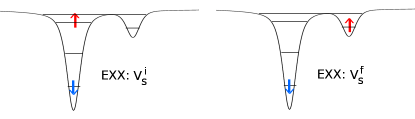
Figure 2: To the left the EXX potential $v_{\scriptscriptstyle\rm S}^{\uparrow,i}$ and the initial configuration for the photoexcited KS state; to the right the final EXX potential $v_{\scriptscriptstyle\rm S}^{\uparrow,f}$ and the target CT state are plotted. Here the position of the arrow denotes where most of the density sits. The model is specified in Section IV.1. As discussed in the text for this photoexcited CT dynamics the EXX potential the transferring $\uparrow-$electron experiences (in the absence of time-dependent external fields) is nearly constant.

The interacting system is prepared in an excited eigenstate of the unperturbed Hamiltonian and then evolved in the presence of a weak monochromatic laser resonant with the photoexcited-to-CT transition frequency $\omega_{CT}$. The latter corresponds to the energy difference between the initial photoexcited state, denoted by $i$, and the final target CT state, denoted $f$, $\omega_{CT}=E_{f}-E_{i}=0.289$ a.u.. The parameters are chosen such that Rabi oscillations between the photoexcited and the CT states are induced (although other states get lightly populated). The exact interacting dynamics is compared with the results from the various TDDFT approximations. For the latter, the initial state is obtained by promoting a KS particle from the ground state configuration to an unoccupied orbital (see the left-hand side of Fig. 2), such that the dominant configuration of the interacting initial state is mimicked. This KS excited state is then relaxed via an SCF calculation to be the KS eigenstate of the initial KS potential $v_{\scriptscriptstyle\rm S}^{(0)}({\bf r},0)$, which prevents any dynamics before the applied field is turned on. The KS system is propagated in the presence of a weak laser resonant with the TDDFT CT resonance of the given approximate functional computed via linear response around the initial KS photoexcited state. (As is common practise, spin-polarized dynamics is run from the initial singly-excited KS determinant). We note that if Condition 2 is violated, this value of the CT resonance is not the value determined from the usual linear response around the ground state, nor is it the value determined from linear response around the target CT state. In fact, as pointed out in Ref. Fuks et al. (2015), the deviation of the resonance predicted from linear response around the initial state, $\omega_{i}$, to that from target state, $\omega_{f}$, is strongly correlated with the performance of the functional approximation. For example, for the two functionals we present here, for EXX $\omega^{i}=\omega^{f}=0.287$a.u. while for SIC-LSD $\omega^{i}=0.287$a.u. and $\omega^{f}=0.237$a.u.. Accordingly, we found in Ref. Fuks et al. (2015) that EXX demonstrated near-perfect charge-transfer, while SIC-LSD began promisingly but ultimately failed to transfer the charge. (Ref. Fuks et al. (2015) also considered LSD, whose discrepancy between the frequencies determined from the initial and target state responses was even greater, and its dynamics was even worse). For the same cases, we demonstrate here explicitly the violation of Condition 1, namely the unphysical time-dependence of the resonance positions, as a function of $\mathcal{T}$.

At various times $\mathcal{T}$ during the evolution we turn off the monochromatic laser and perform a linear density-response calculation to obtain the spectra at these times. The latter is done by applying a delta-kick Yabana et al. (2006) right after the laser is turned off, followed by a free evolution of some duration $T$ and then Fourier transforming the ensuing dipole difference between the kicked and un-kicked free propagations Raghunathan and Nest (2012a); De Giovannini et al. (2013); Oliveira et al. (2015)

$$\Delta d(t)=d^{\mathrm{kicked}}(t)-d^{\mathrm{un-kicked}}(t)\,.$$ (26)

We then plot the dipole spectrum $|\Delta d(\omega)|$, denoted the “absolute spectrum”,

$$|\Delta d(\omega)|=|\int\!\mathop{}\!\mathrm{d}t\,e^{-i\omega t}\Delta d(t)|\,,$$ (27)

We evolved the field-free system for $T=5000~{}a.u,$, resulting in a frequency-resolution of $2\pi/T\approx 0.001$ a.u.. We plot the absolute spectrum $|\Delta d(\omega)|$ instead of the absorption spectrum $Im[d(w)]$ to simplify the analysis, since here we are only analyzing the position of the spectral peaks, not their oscillator strengths.

Fig. 3 shows the spectra for the exact, EXX, and SIC-LSD cases, each driven at their respective initial response frequencies $\omega^{i}$, at different times $\mathcal{T}=0,400,800,1200$ a.u. of the photoexcited CT dynamics shown in the inset. As expected, the exact CT resonance peak only changes strength, but does not shift in position, remaining at $0.289$ a.u. (see upper panel Fig. 3). Note that the exact is obtained from solving the interacting Schrödinger equation and coincides with TDDFT with the exact functional, which satisfies all 3 Conditions.

We had seen in Ref. Fuks et al. (2015) that EXX fulfills Condition 2 in this case, although the resonance position is off by about $0.002$ a.u. from the exact. Here we show explicitly in the middle panel of Fig. 3 that EXX for this dynamics also satisfies Condition 1; in fact even its peak strength changes in a similar way to the exact functional (see middle panel Fig. 3).

SIC-LSD is shown in the lower panel of Fig. 3: peak-shifting signifying violation of Condition 1 is observed as a function of $\mathcal{T}$. The resulting incomplete CT dynamics is evident in the inset.

Figure 3: Logarithm of absolute spectrum $|\Delta d(\omega)|$ Eq. (27) showing CT frequency for different laser durations $\mathcal{T}$. Inset: dipole moments $|d(t)|$ for the photoexcited CT dynamics studied in Ref. Fuks et al. (2015). Upper panel: Exact. Middle panel: EXX. Lower panel: SIC-LSD.

We note that the SIC-LSD peak drifts towards lower frequencies as the charge begins to transfer in time, retracing its path as the charge returns to the donor. That the peak tracks the instantaneous dynamics is not unexpected, given the adiabatic nature of the approximation. The direction of the peak shift (i.e. towards lower frequencies) appears to be consistent with the fact that the linear response frequency computed at the target state, which gets partially occupied during the dynamics, is lower ($\omega^{f}=0.237$ a.u.) than that computed at the initial state ($\omega^{i}=0.287$ a.u., see Table 1).

One might ask what happens to the positions of the other resonances (transitions from the photoexcited state to other unoccupied states) during the dynamics. In Fig. 4 a few peaks corresponding to excitations to higher delocalized states are analyzed as a function of $\mathcal{T}$. For the exact dynamics the positions of the peaks do not change, but as the target CT state gets populated new peaks appear in the spectra, corresponding to transitions from the CT state. The same is true for EXX which is shown in the middle panel of Fig. 4. This is consistent with the observation that EXX satisfies the exact condition. As explained in Ref. Fuks et al. (2015), this is because once the laser is turned off, the KS potential for the transfering electron within EXX is constant.

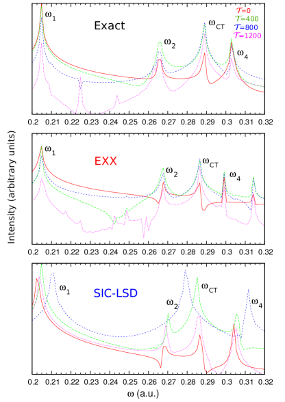
Figure 4: Logarithm of absolute spectrum $|\Delta d(\omega)|$ Eq. (27) for different laser durations $\mathcal{T}$ corresponding to the photoexcited CT dynamics shown in insets of Fig. 3. Upper panel: Exact. Middle panel: EXX. Lower panel: SIC-LSD. Exact and EXX have constant positions for all shown resonances, while SIC-LSD has spuriously time-dependent resonances. For SIC-LSD, $\omega_{2}$ peak shifts up in energy as the system evolves while the $\omega_{\mathrm{CT}}$ shifts down, resulting in one unique broader peak for $\mathcal{T}=800$ a.u. (see Fig. 5 and Table. 1).

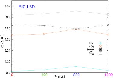
Figure 5: SIC-LSD resonances for different laser durations $\mathcal{T}=0,400,800,1200$ a.u.. $\omega_{1}$, $\omega_{2}$ and $\omega_{4}$ shift up as charge transfers, but $\omega_{CT}$ moves down. It can be seen in table 1 that the direction of the shift is towards the value of each resonance at the final target state. For $\mathcal{T}=800$a.u. $\omega_{2}$ and $\omega_{CT}$ resonances become degenerate, resulting in the overlap of the two peaks (see lower panel Fig. 4). All the resonances return to their initial positions as the dipole moment $d(t)$ shown in inset lower panel Fig. 3 returns to its initial value.

For SIC-LSD shown in lower panel of Fig. 4 not only the CT resonance but also the other peaks corresponding to transitions from the initially photoexcited state to other unoccupied states shift in time. The direction of the shift during the transfer (from $\mathcal{T}$=0 to about $\mathcal{T}$= 800 au) is again towards the positions computed from the final target CT state (see Table 1 last column), and then they shift back as the charge returns, as can be seen in Table 1. In the table, the SIC-LSD response frequencies computed using a $\delta$-kick at different $\mathcal{T}$ for a few transitions lying close to the CT peak are tabulated. The last column shows the values of the resonances computed applying a strong kick in the target SCF CT state. The $\omega_{2}$ transition shifts up in energy and in the target configuration it lies higher in energy than the CT resonance, thus these two transitions cross as the system evolves becoming degenerate at $\mathcal{T}=800$ a.u.(see Fig. 5).

These resonant frequencies can also be computed from linear response around the SCF CT state, by shifting the transition frequencies from this state to the relevant unoccupied states by the value of the transition frequency between the CT and the locally excited state (see Table 2). That is, this table is a check on the ”consistency” statement in Condition 2. We have checked that the exact functional and EXX give identical numbers for the second and third columns, but as evident in Table 2, SIC-LSD shows some deviation from consistency. It is interesting to note that the frequencies obtained from the shifted linear-response TDDFT calculations in column 3 of Table 2 are close to, but not equal, to those obtained by the second-order response calculation in the last column in Table 1. One can also check the consistency statement for excitations out of the CT state (3rd excited state), by shifting the linear-response TDDFT frequencies using the photo-excited state (4th state) as reference. This is shown in Table 3. It is evident that the consistency statement is more significantly violated in this case. Consistency condition is likely to be violated whenever Condition 2 is significantly violated.

SIC-LSD	$\mathcal{T}=0$	$\mathcal{T}=400$	$\mathcal{T}=800$	$\mathcal{T}=1200$	CT target state
$\omega_{1}$	0.202	0.205	0.211	0.204	0.251 $\pm$ 0.003
$\omega_{2}$	0.268	0.270	0.279	0.269	0.314 $\pm$ 0.003
$\omega_{CT}$	0.286	0.285	0.279	0.286	0.236 $\pm$ 0.003
$\omega_{4}$	0.304	0.306	0.311	0.305	0.352 $\pm$ 0.003

Table 1: SIC-LSD resonant frequencies (in atomic units) as computed in the initial locally photoexcited SCF state ($\mathcal{T}=0$) and after the laser has acted for $\mathcal{T}=400,800$ and $1200$ a.u.. The values at each $\mathcal{T}$ were obtained via linear response to a $\delta$-kick perturbation of strength $0.002$ a.u.., for total propagation time $5000$ a.u. and resolution of $0.00125$ a.u., also shown in lower panel Fig. 4. $\omega_{1}$, $\omega_{2}$ and $\omega_{4}$ correspond to excitations from the initial photoexcited state to higher, delocalized states and $\omega_{\mathrm{CT}}$ is a de-excitation to the target CT state. The last column shows the SIC-LSD resonances as computed from the targeted SCF CT state, computed from second order response using a $\delta$-kick perturbation of $0.1$ a.u. strength and evolving for $2000$ a.u., with a resolution of $0.003$a.u. (see text).

SIC-LSD	photoexc. (4th state)	CT (3th state)
$\omega_{1}=\omega_{45}$	0.202	$\omega_{35}-\omega_{34}=0.250$
$\omega_{2}=\omega_{46}$	0.268	$\omega_{36}-\omega_{34}=0.313$
$\omega_{CT}=\omega_{43}$	-0.286	$\omega_{34}=0.237$
$\omega_{4}=\omega_{47}$	0.304	$\omega_{37}-\omega_{34}=0.347$

Table 2: Second column: SIC-LSD resonant frequencies (in atomic units) corresponding to transitions from the initial locally photoexcited SCF state(which corresponds to the 4th excited state) to higher excited states, as computed from the initial photoexcited SCF state (same as shown in second column Table 1). The last column shows the SIC-LSD resonances corresponding to the same transitions but computed via linear response from the targeted SCF CT state(the 3th excited state). (See consistency condition in Section III). The latter are obtained as the difference between the transition frequencies from the SCF CT state to the same final states, after subtraction of the CT resonance as computed at the SCF CT state, namely $\omega_{\mathrm{CT}}=\omega_{34}=0.237$ a.u.

SIC-LSD	CT (3th state)	photoexc. (4th state)
$\omega_{34}$	0.237	$\omega_{43}=-0.286$
$\omega_{35}$	0.487	$\omega_{45}-\omega_{43}=0.489$
$\omega_{36}$	0.550	$\omega_{46}-\omega_{43}=0.554$
$\omega_{37}$	0.584	$\omega_{47}-\omega_{43}=0.590$

Table 3: Second column: SIC-LSD resonant frequencies (in atomic units) corresponding to transitions from the SCF CT state (the 3th excited state) to higher excited states, as computed from the SCF CT state. The last column shows the SIC-LSD resonances corresponding to the same transitions but computed via linear response from the initial locally photoexcited SCF state (the 4th excited state). (See consistency condition in Section III). The latter are obtained as the transition frequencies from the SCF locally excited state to the same final states, after subtraction of the CT resonance as computed at the SCF locally excited state, namely $\omega_{\mathrm{CT}}=\omega_{43}=-0.286$ a.u.

IV.2 Charge-transfer from a Ground State

The TDKS description of long-range CT beginning in a ground state is quite different than that beginning in a photoexcited state. The reason is that when beginning in a ground state the natural choice for the KS initial state is a non-interacting ground state, which is a single-Slater determinant. Such a choice places the transfering electron in a doubly occupied orbital, with the other electron occupying this orbital remaining in the donor. The time-dependent orbital describing the transfering electron must at the same time describe an electron that remains in the donor. The exact KS potential for a model molecule consisting of two closed-shell fragments in its ground state is depicted in Fig. 6. The doubly-occupied orbital initially localized on the donor becomes increasingly delocalized over both the donor and acceptor Fuks et al. (2013a). In the exact xc potential, a step feature develops over time. Approximate functionals can not capture the step, and it is known Fuks et al. (2013a); Raghunathan and Nest (2011); Fuks and Maitra (2014a, b); Hodgson et al. (2013) that they yield poor CT dynamics, failing to transfer the charge, even when the functional yields a good prediction for the CT excitation energy. This is borne out in the dipole dynamics shown in the upper panel Fig. 3 in Ref. Raghunathan and Nest (2011), Fig. 4 in Ref. Fuks et al. (2013a) and upper panel Fig. 1 in Ref. Fuks et al. (2015).

In Ref. Fuks et al. (2015), the failure of the approximate TDDFT dynamics was analyzed from the viewpoint of the violation of Condition 2 using a simple two-electron model and focusing on the EXX approximation. The argument there also goes through for commonly used functionals. Essentially, even when the CT excitation frequency, as determined by linear response from the ground state is accurate, the CT frequency as determined by linear response from the target CT state is poor – in fact it is vanishing, due to static correlation, with delocalized antibonding type of orbitals lying near the delocalized bonding-type of orbital. In the target CT state, the bare KS frequency becomes very small, and so does the approximate $f_{\scriptscriptstyle\rm XC}$-correction, resulting in large violations of Condition 2 by available functionals, $\omega^{i}>>\omega^{f}$. The dynamics is consequently very poor, yielding practically no CT, and very little dynamics occurs except at very short times. Although Condition 2 is strongly violated, the lack of dynamics means that actually Condition 1 is satisfied; since there is very little change in the density, $v_{\scriptscriptstyle\rm XC}(t)$ remains about constant and so do the time-dependent spectra. This example highlights the importance of considering both conditions together when understanding and predicting the performance of approximate functionals.

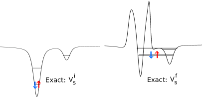
Figure 6: To the left the exact KS potential and initial KS ground state; to the right the exact final KS potential and target CT state are plotted. The model is specified in Section IV.1. As discussed in the text for the CT dynamics starting in the ground state the choice of a SSD forces the occupied time-dependent KS orbital to describe both the electron that transfers to the acceptor, and the electron that remains in the donor. The degeneracy between the bonding and antibonding orbitals in the target CT state is related to the building up over time of a CT step in the exact xc potential Fuks et al. (2013a).

It is also interesting to analyse Condition 3 in this example. Let’s imagine running the same CT dynamics discussed above but backwards, i.e. starting in the CT state and targeting the ground state. We could choose as initial state a doubly occupied orbital, in which case, for a stretched molecule, the bare KS eigenvalue difference $\omega_{\scriptscriptstyle\rm S}$ becomes very small due to the degeneracy between bonding and antibonding orbitals. The EXX kernel together with the Hartree contribution, $f_{\scriptscriptstyle\rm HX}$, equals half Hartree in this case, and the predicted resonance is very small and inaccurate, since the EXX kernel can not correct the vanishing $\omega_{\scriptscriptstyle\rm S}$. On the other hand, we could choose as initial state a spin-broken configuration where $\uparrow$ and $\downarrow$ electrons occupy different orbitals as we did for the photoexcited CT dynamics studied in Section IV.1. Such choice of KS initial state has a finite bare KS eigenvalue difference $\omega_{\scriptscriptstyle\rm S}$, and despite vanishing of the EXX kernel correction within SPA as discussed in Appendix A, EXX gives a reasonably accurate prediction of the physical resonance ($0.287$ au). This example illustrates how two distinct choices of KS initial state can lead to two different predictions of the TDDFT resonance, signifying violation of Condition 3.

IV.3 Adiabatically-Exact Propagation

To assess the impact of the adiabatic approximation itself on the fulfillment of the exact conditions, we now consider propagating self-consistently using the exact ground state xc functional. This “adiabatically-exact” (AE) approximation Thiele et al. (2008), $v_{\scriptscriptstyle\rm XC}^{\mathrm{AE}}[n;\Psi_{0},\Phi_{0}](t)=v_{\scriptscriptstyle\rm XC}^{\mathrm{exact-gs}}[n(t)]$, is the best possible ground state approximation to the xc functional, when using explicit density functionals. All discrepancies with the exact dynamics will be due to the adiabatic approximation. Because this involves finding the potential whose ground state density coincides with the instantaneous one at each time-step, it is computationally quite laborious, so we simplify the model here and consider an asymmetric Hubbard dimer Fuks and Maitra (2014a, b), beginning the dynamics in the ground state. The exact ground state functional can be found by Levy-Lieb contrained search within the small Hilbert space Fuks et al. (2013b). In Ref. Fuks and Maitra (2014a, b) an asymmetric Hubbard dimer was used to study CT dynamics from the ground state (see Fig. 7), showing the same trends as CT dynamics in the LiCN molecule Raghunathan and Nest (2011) and in the real-space one-dimensional model systems studied in Refs. Fuks et al. (2013a, 2015). We now consider the dynamics in the light of Condition 1 and Condition 2. Further, we exploit these conditions to apply a modified field that enhances the amount of charge transfered.

The Hamiltonian of the 2-site Hubbard model reads (Fig. 7),

$$\begin{split}\hat{H}=&-T\sum_{\sigma}\left(\hat{c}_{L\sigma}^{\dagger}\hat{c}_{R\sigma}+\hat{c}_{R\sigma}^{\dagger}\hat{c}_{L\sigma}\right)+U\left(\hat{n}_{L\uparrow}\hat{n}_{L\downarrow}+\hat{n}_{R\uparrow}\hat{n}_{R\downarrow}\right)\\ &+\frac{\Delta v(t)}{2}(\hat{n}_{L}-\hat{n}_{R}),\end{split}$$ (28)

where $\hat{c}_{L(R)\sigma}^{{\dagger}}$ and $\hat{c}_{L(R)\sigma}$ are creation and annihilation operators for a spin-$\sigma$ electron on the left(right) site $L(R)$, respectively, and $\hat{n}_{L(R)}=\sum_{\sigma=\uparrow,\downarrow}\hat{c}_{L(R)\sigma}^{{\dagger}}\hat{c}_{L(R)\sigma}$ are the site-occupancy operators. The occupation difference $\langle\hat{n}_{L}-\hat{n}_{R}\rangle=\Delta n$ represents the dipole in this model, $d=\Delta n$, and is the main variable Fuks et al. (2013b); the total number of fermions is fixed at $N=2$. A static potential difference, $\Delta v^{0}=\sum_{\sigma}(v_{L\sigma}^{0}-v_{R\sigma}^{0})$, renders the Hubbard dimer asymmetric. The total external potential $\Delta v(t)$ is given by $\Delta v(t)=\Delta v^{0}+2{\mathcal{E}(t)}$, where the last term represents a tunable electric field applied to induce CT between the sites. An infinitely long-range molecule is represented by $T/U\to 0$. We choose here the static potential difference as $\Delta v^{0}=-1.5$ U, the hopping parameter $T=0.05$ U and the on-site interaction $U=1$ (see also Ref. Fuks and Maitra (2014b)).

Figure 7: Two-site lattice model Eq. (28) used to study a CT starting in the ground state. Initially, the two electrons occupy the site with the deeper on-site potential $v_{L}$, $|\Delta n_{gs}|\approx 2$. The target CT state consists of two open-shell fragments with approximately one electron on each, $|\Delta n_{\rm CT}|\approx 0$.

The KS Hamiltonian has the form of Eq. (28) but with $U=0$ and $\Delta v(t)$ replaced by the KS potential difference,

$$\Delta v_{s}[\Delta n,\Phi(t_{0})](t)=v_{\scriptscriptstyle\rm HXC}[\Delta n,\Psi(t_{0}),\Phi(t_{0})](t)+\Delta v(t).$$ (29)

For a resonant applied field ${\mathcal{E}(t)}=E_{0}\sin\left(\omega_{\mathrm{CT}}t\right)$, with $\omega_{CT}=(E_{\mathrm{CT}}-E_{\mathrm{gs}})=0.5177~{}a.u.$, the interacting system achieves full population of the CT state after half a Rabi cycle (about 128 a.u.), coinciding with a vanishing dipole moment (see inset in upper panel of Fig. 8). AE dynamics is poor (inset in the middle panel) despite the AE resonance being very accurate, $\omega^{AE}_{gs}=0.5187~{}a.u.$ Fuks and Maitra (2014a). We follow an analogous procedure as described in Section IV to compute the linear response after different durations of the applied laser. The time-step used is $0.01$a.u. and the total propagation time is $T=3000$a.u., resulting in a frequency resolution of about $2\pi/T\approx 0.002$ a.u..

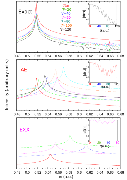
Figure 8: Logarithm of absolute spectrum $|\Delta d(\omega)|$ Eq. (27) showing CT frequency for different laser durations $\mathcal{T}$. Inset: dipole moments $|d(t)|$ for the CT dynamics starting in the ground state studied in Refs. Fuks and Maitra (2014a, b). Upper panel: Exact. Middle panel: AE. Lower panel: EXX.

Fig. 8 upper panel shows the exact dipole response $|\Delta d(\omega)|$ for different $\mathcal{T}$. As expected the position of the peak is constant at $\omega_{CT}$ for all $\mathcal{T}$. In the middle panel of Fig. 8 the AE response for the corresponding $\mathcal{T}$ is shown. Peak-shifting as function of the laser duration $\mathcal{T}$ is noticeable, with clear violation of Condition 1. As time evolves, the density starts transferring to the other site and the KS potential Eq. (29) follows the changes in the density. The AE xc kernel is also time-dependent, but does not have the correct time-dependence to maintain fixed resonance positions. The changes in the AE peak position follow the evolution of the density $\Delta n(t)$ (compare peak migration in lower panel of Fig. 8 with evolution of AE dipole shown in the inset). The AE peak shifts towards higher energies, this is consistent with our findings of Section IV.1, since here $\omega^{f}>\omega^{i}$ Fuks and Maitra (2014b) and thus the peak shift is in the direction of the resonance computed at the final state.

In the lower panel of Fig. 8 the EXX spectra at different $\mathcal{T}$ is shown. The EXX peak shifts as the electron starts transferring and returns to its initial ground state position as the density $\Delta n$ localizes back on the donor site around $\mathcal{T}=60$ a.u. (see inset lower panel of Fig. 8). As the density transfers, the EXX peak shifts towards higher energies, although $\omega^{EXX}_{CT}=\omega^{f}\to 0$. Thus, in this case, the EXX peak does not shift towards $\omega^{f}$. Instead, it is consistent with the peak-shift directions observed in Ref. Provorse et al. (2015), where the instantaneous spectra of small, closed-shell, laser-driven molecules beginning in their ground-state, was studied. There, a single peak was observed in the TDDFT spectra that, as the system transitions onto a single-excited state migrates towards the value of the de-excitation energy from the doubly-excited state to the single-excited state.

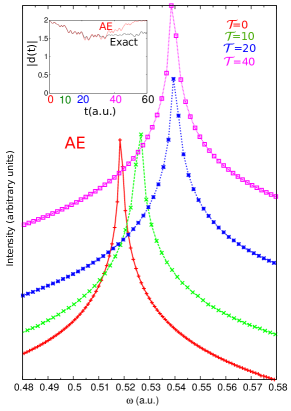
Figure 9: Logarithm of absolute AE spectrum $|\Delta d(\omega)|$ showing CT resonance for different laser durations $\mathcal{T}$. Inset: dipole moments $|d(t)|=|\Delta n(t)|$ for exact (black) and AE (red) for an applied laser ${\cal E}(t)=1.8\sin(0.618t)$ starting in the ground state.

In Fig. 9 we present the AE response $|\Delta d(\omega)|$ for non-resonant dynamics starting in the ground state. The applied laser is detuned by $0.1$a.u. from $\omega^{AE}_{gs}$ (which for this problem as discussed before is very accurate) and is chosen $20$ times stronger than the one applied in the resonant CT dynamics of Fig. 8. The exact dynamics is shown in the inset of Fig. 9 in black, along with the AE dynamics, shown in red in the inset. As expected for the exact dynamics, the position of the CT peak is constant and only the intensity varies (not shown here). Again AE presents spurious time-dependent CT resonance as a function of $\mathcal{T}$, signifying violation of Condition 1. This example of non-resonant dynamics is presented to stress the fact that spurious peak shifting within TDDFT is not exclusive to resonant dynamics.

We next consider an example that violates Condition 1 but satisfies Condition 2, unlike the previous examples: resonant dynamics for a weakly-correlated ($T=U=1$), homogeneous ($\Delta v^{0}=0$) Hubbard dimer Fuks et al. (2013b). Due to symmetry of the Hamiltonian, the ground-state and first-excited densities are identical, $\Delta n_{gs}=\Delta n^{*}$. Condition 2 is satisfied within AE if we start the dynamics in the ground state and target the first local excitation, namely $\omega^{i}_{AE}=\omega^{f}_{AE}$, since the density of both stationary states is the same. The AE dynamics however deviates from the exact as is shown in Ref.Fuks et al. (2013b) and this is due to violation of Condition 1. Linear response calculations at different moments $\mathcal{T}$ for resonant Rabi oscillations show significant peak-shifting, e.g. $\omega^{AE}_{gs}=2.6~{}a.u.$, $\omega^{AE}(\mathcal{T}=15)=2.3~{}a.u.$.

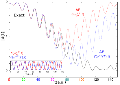
Figure 10: Exact CT dynamics starting in the ground state (black). The AE dynamics in the presence of the monochromatic laser is shown in red. AE dynamics in the presence of the chirped laser, which every $20~{}$a.u. is adjusted to the instantaneous AE resonance $\omega^{AE}(\mathcal{T})$ shown in middle panel Fig. 8, is shown in blue. Inset: monochromatic laser ${\mathcal{E}(t)(\omega_{gs}^{AE},t)}=0.09\sin\left(0.518t\right)$ in red, chirped laser Eq. (30) in blue.

Finally we present a proof of principle directly demonstrating the effect of the spurious time-dependence of the electronic spectra on the TDDFT dynamics. Peak-shifting as the system evolves means that the instantaneous TDDFT resonance is continuously detuned from the TDDFT resonance computed by perturbing the initial state. But what if we would adjust for this spurious detuning by making the applied laser frequency-dependent, i.e. by designing a chirped laser that adjusts its frequency according to changes in the evolving density in order to stay tuned with the instantaneous TDDFT resonance of the KS system?

In Fig. 10, we show the results of propagating the AE system in the presence of a laser whose frequency is adjusted piecewise-in-time during the evolution to be approximately resonant with the KS system; that is every $20$a.u., the frequency of the laser is changed such to be resonant with the instantaneous AE CT resonances shown in middle panel of Fig. 8.

$${\cal E}[\omega^{AE}(\mathcal{T})](t)=0.09\sin\left(\omega^{AE}(\mathcal{T})~{}t\right),$$ (30)

The chirped laser, Eq. (30), is shown in blue in the inset of Fig. 10, as a guide the monochromatic ${\mathcal{E}(t)}=0.09\sin\left(0.518t\right)$ is plotted on top in red. In Fig. 10 the exact dipole dynamics $\Delta n(t)$ is in black, the AE dynamics under the monochromatic laser is in red and the AE dynamics under the chirped laser is in blue. An improvement of the AE dynamics is observed for the laser that is approximately “optimally tuned” in the way above. Notice that for the instantaneous resonances $\omega^{AE}(\mathcal{T})$ in Eq. (30) we have simply used the ones computed for the monochromatic driven AE dynamics of Fig. 8. Further improvements and eventually agreement with the exact dynamics is expected if the chirped laser is designed in a self-consistent way, i.e. if $\omega^{AE}(\mathcal{T})$ would be computed for the AE evolution in the presence of the chirped laser.

V Conclusions and Outlook

Recent observations of time-dependent spectra in TDDFT(or TDHF) have drawn much attention: Unphysical shifts in the position of their spectral peaks have been reported for electron dynamics far from equilibrium Ramakrishnan and Nest (2012); Raghunathan and Nest (2012a); De Giovannini et al. (2013); Habenicht et al. (2014); Fuks et al. (2015); Provorse et al. (2015); Oliveira et al. (2015); Fischer et al. (2015). Peak shifting is expected for coupled electron-ion dynamics or when computing resonances in the presence of time-dependent fields, but once all time-dependent fields are turned off electronic resonance positions are constant for pure electron dynamics. The cancellation of spurious time-dependence to yield constant resonances has been rationalized as an exact condition for the xc functional of TDDFT in Ref. Fuks et al. (2015). In this article we have elaborated on the theoretical aspects of the formulation and provided a detailed study of some representative examples that illustrate the relevance of the exact condition for the dynamics.

A generalized non-equilibrium response function was derived which applies to general non-equilibrium situations when the external fields are off Fuks et al. (2015); Perfetto and Stefanucci (2015). In contrast to the standard linear response formalism applied to systems around the ground state, the generalized non-equilibrium response function $\tilde{\chi}[n^{(0)}_{\mathcal{T}};\Psi(\mathcal{T})]$ deals with non-stationary densities $n^{(0)}_{\mathcal{T}}$ in the absence of time-dependent fields and is not time-translationally invariant. We showed that due to the lack of this symmetry the frequency-dependent response $\tilde{\chi}_{t^{\prime}}({\bf r},{\bf r}^{\prime},\omega)$ or $\tilde{\chi}_{T}({\bf r},{\bf r}^{\prime},\omega)$ depends parametrically on a time-variable $t^{\prime}$ or $T=(t+t^{\prime})/2$, respectively, and each exhibits a different pole structure. The density response $\delta n({\bf r},\omega)$ is independent of this choice as it should be. The latter has poles at the physical resonances of the system, corresponding to transitions between eigenstates of the unperturbed Hamiltonian.

By virtue of the Runge-Gross theorem Runge and Gross (1984) the exact time-dependent KS system reproduces the non-equilibrium density response $\delta n({\bf r},\omega)$ exactly. Therefore, a Dyson-like equation connects $\tilde{\chi}[n^{(0)}_{\mathcal{T}};\Psi(\mathcal{T})]$ with the non-equilibrium KS response $\tilde{\chi}_{\scriptscriptstyle\rm S}[n^{(0)}_{\mathcal{T}};\Psi(\mathcal{T}),\Phi(\mathcal{T})]$ via a generalized kernel $\tilde{f}_{\scriptscriptstyle\rm HXC}[n^{(0)}_{\mathcal{T}};\Psi(\mathcal{T}),\Phi(\mathcal{T})]$. A simple Lehmann representation can be written down for $\tilde{\chi}$ but not for $\tilde{\chi}_{\scriptscriptstyle\rm S}$ because the KS potential is not static for non-stationary densities $n^{(0)}_{\mathcal{T}}$.

The exact condition was formulated in several different ways. In the language of pump-probe experiments, the resonance positions must be independent of the moment $\mathcal{T}^{\prime}$ the pump is turned off and of the delay $\theta$ between pump and probe. More generally, in the absence of ionic motion, the TDDFT response frequencies (corresponding to transitions between two given interacting states) of a field-free system must be independent of the interacting state $\Psi(\mathcal{T})$ around which the response is calculated (Condition 1). When the interacting system is in any excited stationary state, and the KS reference state is also chosen to be a stationary state of its potential, we can formulate the exact condition in a matrix form. In such a case, the TDDFT resonance frequency for a specific transition between two stationary states must be independent of which of the two states the response is calculated around (Condition 2). Further, a consistency condition relates the frequencies of transitions to other states from each reference state. The TDDFT response frequencies must be invariant also with respect to the choice of KS state (Condition 3). The exact conditions pose a very challenging task for the xc kernel, as we illustrated with several examples.

The first example was that of CT dynamics from a photo-excited state. We used a model system of two electrons in an asymmetric double-well and started the KS propagation with one orbital promoted to a locally excited orbital; this electron was then driven to the other well by means of a weak resonant field. The performance of the different functionals to accurately simulate this dynamics was related to the fulfillment of the exact condition in its different forms. In Ref. Fuks et al. (2015) it was observed that the degree of violation of Condition 2 was directly related to the performance of the approximate functional to reproduce the dynamics. Here the time-dependent spectra for the same approximated functionals, including EXX and SIC-LSD are compared against the exact calculation at different moments in the evolution. We find that in addition to Condition 2 also Condition 1 was violated within SIC-LSD, resulting in spurious peak shifting and consequently in poor dynamics. The CT peak moved towards the SIC-LSD resonance computed around the final target state and this trend held also for the other resonances of the system. SIC-LSD resonances were also shown to violate the consistency condition. Unrestricted EXX was shown to fulfill Condition 2 for this particular case Fuks et al. (2015) and here we showed it also has fixed peak positions along the evolution (fulfillment of Condition 1), resulting in very accurate photoexcited CT dynamics.

In the next example, CT dynamics starting in the ground state, EXX trivially fulfilled Condition 1 but violated Condition 2, resulting in poor dynamics. We also briefly discussed the violation of Condition 3 by EXX when we consider different initial KS states when running the dynamics backwards beginning in the CT state.

In order to assess the impact of the adiabatic approximation alone, independent of the effect of the choice of approximate ground-state functional, we used a two-site lattice model. Given the small Hilbert space the exact ground state xc functional can be found Fuks et al. (2013b) and was used to self-consistently propagate the KS system (AE propagation). We tuned the parameters of the system to mimic long-range CT dynamics starting in the ground state Fuks and Maitra (2014a, b). We observed that the AE CT dynamics violates both Condition 1 and Condition 2 and resulted in poor dynamics. Violation of Condition 1 was observed for AE for both resonant and also off-resonant dynamics. In the case of the weakly-correlated homogeneous Hubbard model studied in Ref. Fuks et al. (2013b) Condition 2 was satisfied but Condition 1 was violated within AE, resulting in inaccurate dynamics.

Perhaps the clearest impact of the influence of the exact condition on the dynamics was illustrated by the “optimally tuned” laser that adjusted in a piece-wise manner to the instantaneous AE resonance (Figure 10 and discussion). This showed that the AE propagation in the presence of this chirped laser resulted in an improved charge transfer rate in the case of resonant CT dynamics.

We conclude that in order to be able to predict the performance of a given approximate functional all three Conditions need to be considered. Further because the best possible ground state approximation for the density-functional fails to fulfill the exact conditions, resulting in poor dynamics, we stress the need to go beyond the adiabatic approximation.

We have shown the large impact that the violation of the exact conditions has on the ability of approximate functionals to reproduce the dynamics: the higher the degree of the violation, the poorer the simulated dynamics. The examples presented here are drastic, but we have only analyzed small systems, perhaps a worst-case scenario for approximate TDDFT. An important question for future work is the system-size scaling of the violation of the exact conditions. When ionic motion is considered, the spectral peaks can be vibrationally broadened, perhaps relaxing the stringent exact conditions discussed here. Development of an approximate functional or a propagation scheme that fulfills exactly or approximately the exact conditions is an important direction for future research.

Appendix A $f_{\scriptscriptstyle\rm HXC}$ correction in EXX within the Single Pole Approximation

Within the single-pole approximation using EXX it can be shown that for a two-electron singlet state where the two electrons occupy different spatial orbitals, the $f_{\scriptscriptstyle\rm HXC}$ correction vanishes. First, note the definition of the spin-resolved xc kernel Petersilka et al. (1996); Grabo et al. (2000),

$$f_{\scriptscriptstyle\rm XC}^{\sigma\sigma^{\prime}}({\bf r},{\bf r}^{\prime},t,t^{\prime})=\frac{\delta v_{\scriptscriptstyle\rm XC}^{\sigma}({\bf r},t)}{\delta n_{\sigma^{\prime}}({\bf r}^{\prime},t^{\prime})}$$ (31)

In adiabatic EXX, $v_{\scriptscriptstyle\rm XC}^{\sigma}[n_{\uparrow},n_{\downarrow}]({\bf r})=v_{\scriptscriptstyle\rm X}^{\sigma}[n_{\uparrow},n_{\downarrow}]({\bf r})=\frac{\delta E_{\scriptscriptstyle\rm X}[n_{\uparrow},n_{\downarrow}]}{\delta n_{\sigma}({\bf r})}$, where for two electrons

$$E_{\scriptscriptstyle\rm X} = -\frac{1}{2}\sum_{\sigma=\uparrow,\downarrow}\sum_{ij}^{N_{\sigma}}\int\!\!\int\frac{\phi_{i\sigma}({\bf r})\phi_{i\sigma}({\bf r}^{\prime})\phi_{j\sigma}({\bf r}^{\prime})\phi_{j\sigma}({\bf r})}{|{\bf r}-{\bf r}^{\prime}|}\mathop{}\!\mathrm{d}{\bf r}\mathop{}\!\mathrm{d}{\bf r}^{\prime}$$ (32)

$$= -\frac{1}{2}\sum_{\sigma=\uparrow,\downarrow}\int\!\!\int\frac{n_{\sigma}({\bf r})n_{\sigma}({\bf r}^{\prime})}{|{\bf r}-{\bf r}^{\prime}|}\mathop{}\!\mathrm{d}{\bf r}\mathop{}\!\mathrm{d}{\bf r}^{\prime}$$

$$= -E_{\scriptscriptstyle\rm H}[n_{\downarrow}]-E_{\scriptscriptstyle\rm H}[n_{\uparrow}]\;.$$

This yields $v_{\scriptscriptstyle\rm X}^{\sigma}[n_{\uparrow},n_{\downarrow}]=-v_{\scriptscriptstyle\rm H}[n_{\sigma}]$, and so using Eq. 31,

$$f_{\scriptscriptstyle\rm XC}^{\downarrow\uparrow}=f_{\scriptscriptstyle\rm XC}^{\uparrow\downarrow}=0\;\;{\rm while}\;\;f_{\scriptscriptstyle\rm XC}^{\uparrow\uparrow}=f_{\scriptscriptstyle\rm XC}^{\downarrow\downarrow}=-f_{\scriptscriptstyle\rm H}$$ (33)

Thus for the parallel spin case the Hartree-exchange kernel $f_{\scriptscriptstyle\rm HX}^{\sigma\sigma}=0$ vanishes, however in the case of anti-parallel spin $f_{\scriptscriptstyle\rm HX}^{\uparrow\downarrow}=f_{\scriptscriptstyle\rm HX}^{\downarrow\uparrow}=f_{\scriptscriptstyle\rm H}$.

Now for a non-degenerate Kohn-Sham pole, $\omega_{\scriptscriptstyle\rm S}=\epsilon_{a}-\epsilon_{i}$, the single-pole approximation for the TDDFT excitation energy depends only on the parallel-spin component of the kernel Petersilka et al. (1996); Grabo et al. (2000):

$$\omega=\omega_{\scriptscriptstyle\rm S}+\int\Phi_{q}({\bf r})\left(f_{\scriptscriptstyle\rm H}+f_{\scriptscriptstyle\rm XC}^{\sigma\sigma}\right)\Phi_{q}({\bf r}^{\prime})d{\bf r}d{\bf r}^{\prime}$$ (34)

(where, as before, $\Phi_{q}({\bf r})=\phi_{i}({\bf r})\phi_{a}({\bf r})$), clearly yielding a zero correction for the case of adiabatic EXX. That is, within the single-pole approximation, the KS response frequencies are identical to the TDDFT excitations when the two electrons are occupying different orbitals (see Section IV.1). In contrast, when they occupy the same spatial orbital, as for a spin-saturated two-electron singlet (see section IV.2), each Kohn-Sham pole is doubly-degenerate, and Eq. 34 is modified, see Ref. Petersilka et al. (1996); Grabo et al. (2000) for details; the kernel correction in EXX, $f_{\scriptscriptstyle\rm X}=-f_{\scriptscriptstyle\rm H}/2$, does not vanish for this case.