The scaling of boson sampling experiments

Abstract

Boson sampling is the problem of generating a quantum bit stream whose average is the permanent of a $n\times n$ matrix. The bitstream is created as the output of a prototype quantum computing device with $n$ input photons. It is a fundamental challenge to verify boson sampling, and the question of how output count rates scale with matrix size $n$ is crucial. Here we apply results from random matrix theory to establish scaling laws for average count rates in boson sampling experiments with arbitrary inputs and losses. The results show that, even with losses included, verification of nonclassical behaviour at large $n$ values is indeed possible.

Much recent attention has been given to the application of multichannel linear photonic networks to solving computational tasks thought to be inaccessible to any classical computer. Such devices are the prototypes of quantum computers Knill et al. (2001); Kok et al. (2007) and novel metrology devices O’Brien et al. (2009); Motes et al. (2015a). Exponentially hard problems that are not soluble with digital classical technology have many potential applications Papadimitriou . In particular, “BosonSampling” Aaronson and Arkhipov (2011, 2013) is the hard problem of how to generate a bitstream of photon-counts with the distribution of a unitary or Gaussian permanent. This result is created as the output from a single photon input to each of $n$ distinct channels. This is conjectured to be exponentially hard at large $n$, while being relatively straightforward to implement physically.

It is widely appreciated that to verify the solution is correct is an important and significant challenge Aaronson and Arkhipov (2014); Carolan et al. (2014); Spagnolo et al. (2014); Gogolin et al. (2013); Bentivegna et al. (2015); Aolita et al. (2015); Tichy et al. (2014); Bentivegna et al. (2016). The task is to measure the coincidence rates of counting $n$ photons in $n$ output channels and to confirm that they correspond to the modulus squared of an $n\times n$ sub-permanent of a unitary matrix. The matrices are under experimental control Broome et al. (2013); Crespi et al. (2013); Tillmann et al. (2013); Spring et al. (2013), and an average over a random ensemble of them is necessary to verify the experiments. A number of known strategies exist.

Yet, since permanents are intrinsically exponentially hard to compute Valiant (1979), it is nontrivial to verify the output is correct Aaronson and Arkhipov (2013, 2014) at large $n$ values. This computational issue makes it difficult to estimate how count rates scale unless averaged over all unitaries. Understanding scaling is essential because count rates decline exponentially fast as $n$ increases, requiring a strategy that overcomes this.

In this Letter, we solve the average scaling problem for arbitrary inputs and losses. We obtain the maximum scaling of improvements that are possible with recent channel grouping strategies Carolan et al. (2014). To achieve this, we combine the generalized P-representation with methods from random matrix theory to obtain averages over unitary transformations. This allows to describe realistic photonic network experiments, with arbitrary inputs, outputs, and losses. Such losses in boson sampling have recently been investigated elsewhere Motes et al. (2015b); Aaronson and Brod (2016).

The scaling improvement with channel grouping depends on the channel occupation ratio, $k=m/n$, reaching over a hundred orders of magnitude at $k=6$, $n=100$. This is well beyond the capability of any classical, exact computation of matrix permanents. Our results show that boson-sampling verification with such large $n$ values is possible provided high efficiency detectors are available.

Scaling issues like this arising in random matrix theory are widespread Forrester (2010), as averages over unitaries are fundamental to quantum physics. We note an unexpected analogy with the statistics of a classical device for generating random counts. On averaging over all unitaries, the probability of $n$ single-photon counts in $n$ preselected channels — a quantum Galton’s board Gard et al. (2014) — is identical to a classical Galton’s board. The only difference is that there are now $n-1$ additional virtual channels, which describe multi-photon events in an output mode.

These extra channels can be thought of as non-classical communication channels. Such channel capacity improvements are known from quantum communication theory Caves and Drummond (1994), and are closely related to Arkhipov and Kuperberg’s “birthday paradox” for bosons Arkhipov and Kuperberg (2012).

We start with a result Glauber (1963a); Mandel and Wolf (1995) from quantum optics: any bosonic correlation function is obtainable from the normally-ordered quantum characteristic function,

$$\chi\left(\bm{\xi}\right)=\left\langle:e^{\bm{\xi}\cdot\hat{\bm{a}}^{\dagger}-\bm{\xi}^{*}\cdot\hat{\bm{a}}}:\right\rangle.$$ (1)

Here, $\left\langle\hat{O}\right\rangle\equiv Tr\left[\hat{\rho}\hat{O}\right]$ is a quantum average, which we calculate using a generalized P-representation Drummond and Gardiner (1980). This approach extends the Glauber P-function Glauber (1963b), giving a distribution $P\left(\bm{\alpha},\bm{\beta}\right)$ over are two $m$-component complex vectors, which exists for any $m-$mode bosonic state $\hat{\rho}$. The quantum characteristic is then obtained from Gardiner and Zoller (2000)

$$\chi\left(\bm{\xi}\right)=\int P\left(\bm{\alpha},\bm{\beta}\right)\chi\left(\bm{\xi}|\bm{\alpha},\bm{\beta}\right)d\mu\left(\bm{\alpha},\bm{\beta}\right)\,,$$ (2)

where $d\mu\left(\bm{\alpha},\bm{\beta}\right)$ is the integration measure, and $\chi\left(\bm{\xi}|\bm{\alpha},\bm{\beta}\right)\equiv\exp\left(\bm{\xi}\cdot\bm{\beta}-\bm{\xi}^{*}\cdot\bm{\alpha}\right)$ is the conditional characteristic function for $\bm{\xi}$ given a particular quantum phase-space trajectory $\bm{\alpha},\bm{\beta}$.

Transmission through a linear network changes the input density matrix $\hat{\rho}^{(\mathrm{in})}$ to an output density matrix $\hat{\rho}^{(\mathrm{out})}$. An amplitude transmission matrix $T$ transforms the coherent amplitudes Drummond and Hillery (2014), so that $\bm{\alpha}^{(\mathrm{out})},\,\bm{\beta}^{(\mathrm{out})}=T\bm{\alpha},\,T^{*}\bm{\beta}$. The output characteristic $\chi^{(\mathrm{out})}$ now depends on the input phase-space amplitude $\bm{\alpha},\bm{\beta}$ in an intuitively understandable way:

$$\chi^{(\mathrm{out})}\left(\bm{\xi}|\bm{\alpha},\bm{\beta}\right)=e^{\bm{\xi}\cdot\bm{T}^{*}\bm{\beta}-\bm{\xi}^{*}\cdot\bm{T}\bm{\alpha}}\,.$$ (3)

To calculate the average scaling behavior, we consider the case of $T=\sqrt{t}U$, in which the unitary mode transformation $U$ of the photonic network is combined with an absorptive transmission coefficient $t$, representing losses and detector inefficiencies. We compute the average output correlations over all possible unitaries, indicated by $\left\langle\right\rangle_{U}$, from random matrix theory Fyodorov (2006). This allows one to evaluate averages of exponentials of the unitary matrices in the conditional characteristic function, $\chi^{(out)}$ of Eq. (3).

The result is an averaged conditional characteristic

$$\left\langle\chi^{(\mathrm{out})}\left(\bm{\xi}|\bm{\alpha},\bm{\beta}\right)\right\rangle_{U}=\left(m-1\right)!\sum_{j=0}^{\infty}\frac{\left[-t\left|\bm{\xi}\right|^{2}\bm{\beta}\cdot\bm{\alpha}\right]^{j}}{j!\left(m-1+j\right)!}\,.$$ (4)

Inserting this unitary average in Eq. (2) gives an exact solution for any averaged observable in the photonic network, with arbitrary inputs and losses. The output photon statistics depend on $\bm{\beta}\cdot\bm{\alpha}$, which is the phase-space equivalent of the total input photon number $\hat{N}$. As a result, the characteristic function after unitary and quantum averaging is:

$$\left\langle\chi^{(\mathrm{out})}\left(\bm{\xi}\right)\right\rangle_{U}=\left(m-1\right)!\sum_{j=0}^{\infty}\frac{\left(-t\left|\bm{\xi}\right|^{2}\right)^{j}\left\langle:\hat{N}^{j}:\right\rangle}{j!\left(m-1+j\right)!}\,.$$ (5)

The effect of unitary averaging is such that all output channel and phase information is lost, since the characteristic function now only depends on $\left|\bm{\xi}\right|^{2}$. This also shows that all output averages are obtained solely from the normally ordered input photon number moments, $\left\langle:\hat{N}^{j}:\right\rangle$, regardless of which input channels are used. As a common example, for an input $n$-photon number state $\left\langle:\hat{N}^{j}:\right\rangle=n!/(n-j)!$, so the sum in Eq. (5) vanishes for $j>n$. This is a consequence of photon-number conservation and the purely absorptive loss reservoirs.

Only the photon number observables are non-vanishing after unitary phase-averaging. These are most readily obtained from taking derivatives of the photon-number generating function Cantrell (1971),

$$G\left(\bm{\gamma}\right)\equiv Tr\left(\hat{\rho}\prod_{i}\left(1-\gamma_{i}\right)^{\hat{n}_{i}}\right)\,.$$ (6)

Using the relationship between photon-number generator and characteristic function Rockower (1988), we find that:

$$G\left(\bm{\gamma}\right)\equiv\left(m-1\right)!\sum_{j=0}^{\infty}\frac{\left(-t\right)^{j}\left\langle:\hat{N}^{j}:\right\rangle}{\left(m-1+j\right)!}\sum_{\sum\mathbf{j}=j}\gamma_{1}^{j_{i}}\ldots\gamma_{m}^{j_{m}}$$ (7)

This result is completely general for a photonic network with arbitrary inputs, outputs and losses. A case of special interest is $P_{n|m}$, the probability of observing $1$ photon in each of $n$ channels, given an $n$-photon input and an $m$-mode network. This is found on taking $n$ first derivatives of $G\left(\bm{\gamma}\right)$, so that:

$$P_{n|m}=\frac{t^{n}\left(m-1\right)!n!}{\left(m-1+n\right)!}=t^{n}\left[C_{n}^{m+n-1}\right]^{-1}\,$$ (8)

We now wish to relate these results to the permanent of the transmission matrix $T$. The permanent is a sum over all permutations $\sigma$ of the matrix indices of the product of $n$ terms, in which neither row nor column indices are repeated. It is an exponentially hard object to compute, and is one of the fundamental quantities addressed in boson sampling theory and in linear optical networks Scheel (2005, 2004).

For a pure, unitary state evolution, the photon counting probability is the permanent of a sub-matrix, $\left\langle\left|\mathrm{perm}(U_{n|m})\right|^{2}\right\rangle$, where $U_{n|m}$ is any $n\times n$ sub-matrix of $U$ Aaronson (2011). More generally, we replace $U_{n|m}\rightarrow T_{n|m}$, so as to include losses.

The permanent of a sub-matrix of $T$ is obtainable Li and Zhang (2015) from the permanental polynomial, which has similarities with moment generating function. This is given by:

$$p(x)=\mathrm{perm}(xI-T)\equiv\sum_{n=0}^{m}b_{n}x^{m-n}\,.$$ (9)

Next, we consider how to compute the unitary average of products of the permanents, using$\left\langle.\right\rangle_{U}$ to indicate averages over the circular unitary ensemble, with a Haar measure. This is achieved through an elegant result in random matrix theory Fyodorov (2006). The unitary average of permanental polynomials in Eq. (9) is:

$$\left\langle p(x)p(y)^{*}\right\rangle_{U} = m!(m\text{\textminus}1)!\sum_{j=0}^{m}\frac{t^{j}\left(xy^{*}\right)^{m-j}}{\left(m-j\right)!(m-1+j)!}\,.$$ (10)

If $\omega^{(n)}=(\omega_{1},\ldots\omega_{n})$ where $\omega_{1}<\omega_{2}\ldots<\omega_{n}$, we can define an $n\times n$ sub-matrix $T_{\bm{\omega}}\equiv T_{\omega_{i}\omega_{j}}$. The coefficients of this polynomial are simply the sums over the permanents of all possible distinct sub-matrices:

$$b_{n}=(-1)^{n}\sum_{\bm{\omega}^{(n)}}\mathrm{perm}(T_{\bm{\omega}^{(n)}})\,.$$ (11)

The number of sub-matrices in the sum has a multiplicity given by the binomial coefficient $C_{n}^{m}=m!/\left(n!(m-n)!\right)$, corresponding to the different ways to choose the distinct indices $\omega_{j}$. These indices have a straightforward physical interpretation: they are the channel numbers of the input or output modes of the photonic device.

Expanding the product average, and noting that products of different sub-matrices vanish under unitary ensemble averaging, we consider the sub-permanents with $j=n$. The average sum over all possible sub-permanents of this size is a ratio of two binomial coefficients, which we define as $R_{n|m}$:

$$\sum_{\bm{\omega}^{(n)}}\left\langle\left|\mathrm{perm}(T_{\bm{\omega}^{(n)}})\right|^{2}\right\rangle_{U}=R_{n|m}=\frac{t^{n}m!(m\text{\textminus}1)!}{(m-n)!(m+n-1)!}\,.$$ (12)

All the averages are the same for every sub-matrix. Therefore, we can replace $T_{\bm{\omega}^{(n)}}$ by any particular sub-matrix $T_{n|m}$, and make use of the sub-matrix multiplicity. The final result is the same as in Eq. (8), except expressed using permanents, so that $P_{n|m}=\left\langle\left|\mathrm{perm}(T_{n|m})\right|^{2}\right\rangle_{U}$. In the lossless limit of $t=1$, this result agrees with the “bosonic birthday paradox” of Arkhipov and Kuperberg Arkhipov and Kuperberg (2012), derived using different techniques.

We turn next to some limiting cases for large $n$, where $\log P_{n|m}\approx n\epsilon$ for a scaling exponent $\epsilon$.

Entire matrix

If the matrix is the entire transmission matrix, then $n=m$. The scaling exponent is $\epsilon=\log\left(t/4\right)$, and

$$\log P_{n|m}\,\mathop{\sim}\limits_{n\to\infty}\,\,n\epsilon+\frac{1}{2}\log\left[4\pi n\right]\,.$$ (13)

This result generalizes one of Fyodorov Fyodorov (2006).

Gaussian limit

Next, take $n\ll m$, so that $k\gg 1$. Standard methods for approximating a binomial coefficient in this limit give the scaling exponent $\epsilon=\log\left(t/\left(k+1/2\right)\right)-1$, where $k=m/n$, so that:

$$\log P_{n|m}\,\,\mathop{\sim}\limits_{n\to\infty}\,\,n\epsilon+\frac{1}{2}\log\left[2\pi n\right]\,.$$ (14)

This is consistent with the fact that for large $k$, unitary sub-matrices reduce to matrices with complex Gaussian random entries Jiang (2009); Aaronson and Arkhipov (2013).

General sub-matrix

For the general case, the scaling exponent is $\epsilon=\log t+k\log k-(1+k)\log(1+k)$, and the asymptotic result is:

$$\log P_{n|m}\,\mathop{\sim}\limits_{n\to\infty}\,\,n\epsilon+\frac{1}{2}\log\left[2\pi n(1+1/k)\right]$$ (15)

The exact result is plotted in Figure 1, with different values of $k=m/n$. The power law is so close that it cannot be told apart from the exact result on this scale. For all numerical results, we choose $t=1$, since results in more realistic cases with losses are readily obtained by adding $\log t$ to the scaling exponents.

At large $k$ values, one obtains the Gaussian limit of Eq. (14). This gives an increasingly negative exponent, with exponentially small count-rates.

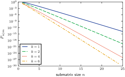
Figure 1: Average sub-unitary permanent squared $P_{n|m}$ with $t=1$ for $k=1,2,4,6$, with $k=1$ at the top and $k=6$ at the bottom.

Next, we show the result of an actual average over a finite, random ensemble with $S=40000$ unitary samples. In the graphs, for $k=m/n=2$ and $n\leq 25$ we give the relative errorWes in the asymptotic approximation and a numerical average, compared to the exact solution. To estimate statistical error-bars, we take an ensemble $S$, and divide it into $\sqrt{S}$ sub-ensembles, giving sub-ensemble means which are approximately Gaussian from the central limit theorem.

These are averaged, and the error in the mean $\sigma_{m}$ is obtained using standard techniques. The error-bars are given in the plots as $\pm\sigma_{m}$. The results agree with the exact equation with a relative error comparable to the sampling error-bars. For the plotted ratio of $k=2$, the errors are around $\pm 1\%$ for over twenty orders of magnitude range of values, and we see that the relative sampling error over unitaries is independent of matrix size for $n\geq 10$.

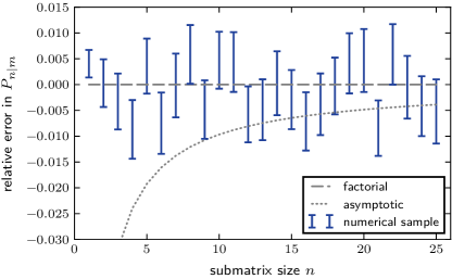
Figure 2: Relative sampling errors in the sub-unitary permanent squared $P_{n|m}$ with $t=1$ for $k=2$. Numerical results for $40,000$ random unitaries (solid lines with error bars) are compared to exact results (dashed lines) and the asymptotic power law form (dotted line) for up to $n=25$.

While the scaling is better than the Gaussian limit of $k\gg 1$, it is still a problem for boson sampling verification. Even in the unlikely case of perfect efficiency, the average permanent for a photon number of $n=24$ is $\sim 10^{-18}$ with a sub-matrix ratio of $k=2$. This is the probability of a coincidence count, so one needs $10^{18}$ samples to obtain one count for a typical unitary. At a repetition rate of $10^{12}\,\mathrm{Hz}$, which is the maximum one can reasonably expect from the technology, one would require $10^{6}\,\mathrm{s}$ of measurement time for each count.

The reason for this is simple: many-body complexity. There are too many quantum states possible. Monitoring the coincidence channels for one many-body state takes too long, even though it is these counts that are of interest. This property, although making verification hard, is the most interesting feature of these experiments. They give a uniquely controllable access to a laboratory system in which one can unravel the complexity of a many-body system, in order to examine each state, or arbitrary combinations of the quantum states.

Accordingly, suppose we consider what happens when one groups multiple output channels together, by using logic gate operations on the detector circuits, as in a recent, pioneering experiment Carolan et al. (2014). A large number of randomized sets of channels can be combined, to obtain a unique distinguishing signature for each unitary.

This strategy has important advantages over previous proposals. It increases count-rates by exponentially large factors, and may allow a test of the unitary output bitstream for matrices with permanents larger than $n=40$, beyond the classical computation limits. Yet, it is not restricted to any particular unitary, reducing the chance that the device may only work in special cases. One can also use the strategy to efficiently test for null counts, in edge cases like Fourier matrices Tichy et al. (2014).

Our scaling laws predict the upper bound of the count-rate gain that can achieved through sub-matrix multiplicity. The upper bound from channel grouping is given by $R_{n|m}$, in Eq. (12). This has an exponent of $\lambda=\log t+2k\log k-(k-1)\log(k-1)-(k+1)\log(k+1)$, so that the scaling is:

$$\log R_{n|m}\,\,\mathop{\sim}\limits_{n\to\infty}\,\,n\lambda+\frac{1}{2}\log\left[\frac{k+1}{k-1}\right]$$ (16)

For the Gaussian limit of $n,k\gg 1$, one finds that $\lambda\rightarrow\log t-1/k$. Unlike the single coincidence case, the grouped channel count rate is maximized for large $k$, rather than minimized as before. The corresponding upper-bound result is plotted in Figure 3, for different values of $k=m/n$, again taking $t=1$ for simplicity.

At at $k=6$, and $n=100$, there is now a dramatic increase of more than $100$ orders of magnitude in total count-rate. The improvement is greatest for large $k$ values, which are the cases of most interest. High $n$ verification still requires total efficiencies of above $90\%$, which is possible as the technology improves.

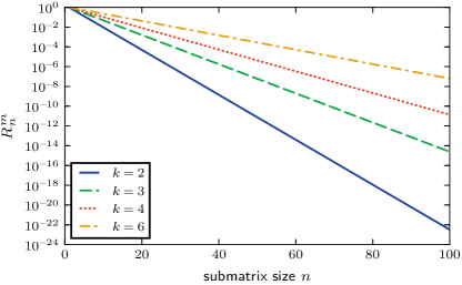
Figure 3: Upper bound on count-rates $R_{n}^{m}$ for $n$ photons occurring, without bunching, in any $n$ output channels, for $k=2,\ldots 6$, with $k=6$ at the top.

It is an intriguing result, mathematically and physically, that the quantum Galton’s board has a close relationship with the binomial coefficients normally found in classical combinatorics. How can we interpret this result?

Suppose that we replaced the photonic network, equivalent to a unitary transformation, by an updated Galton’s board device, which simply switched the photons from the $n$ input channels to the $n$ output channels in a random way. This would not involve interference, and would have a similar behavior to a mechanical board, apart from an increased number of inputs.

Under these conditions, the average probability of all counts occurring in a preselected set of $n$ output channels is an inverse binomial $\left[C_{n}^{m}\right]^{-1}$. We now see a truly remarkable result. Apart from losses, the quantum Galton’s board has, on averaging over all unitaries, identical output coincidence probabilities to a classical Galton’s board with a number of channels given by $\tilde{m}=m+n-1$.

In other words, the fact that photons can bunch — one channel may carry up to $n$ photons, after all — has a similar effect on the output statistics as if the device were classical, but with $n-1$ additional channels available. Needless to say, these virtual channels do not exist. They represent, on average, the additional output possibilities available owing to the fact that several bosons can occupy the same mode, and hence occur in the same channel. This is the large-scale consequence of the famous Hong-Ou-Mandel effect in quantum optics Hong et al. (1987); Walborn et al. (2003).

It is this additional, virtual channel capacity that allows more quantum information to be transmitted in a quantum photonic network than is feasible if each channel was used separately, with one bit per channel. Such extra capacity is a fundamental and important property of quantum photonic networks Caves and Drummond (1994).

In summary, the unitary average of moduli of sub-permanents has remarkable properties. Each permanent itself has no simple closed-form expression, and one might imagine that taking an average over all possible unitaries would only make things harder. Yet the average over the unitary ensemble is just as simple as the closed form expression applicable to a classical Galton’s board.

As well as improved measurements, verification for an individual large unitary requires improved computational methods, as standard methods take exponentially long times. These results will be treated elsewhere. In addition to understanding the scaling laws for verifying boson sampling, our results may suggest how random matrix theory can be applied to other, large-scale quantum technologies.