Optimization via Separated Representations and the Canonical Tensor Decomposition

Abstract.

We introduce a new, quadratically convergent algorithm for finding maximum absolute value entries of tensors represented in the canonical format. The computational complexity of the algorithm is linear in the dimension of the tensor. We show how to use this algorithm to find global maxima of non-convex multivariate functions in separated form. We demonstrate the performance of the new algorithms on several examples.

1. Introduction

Finding global extrema of a multivariate function is an ubiquitous task with many approaches developed to address this problem (see e.g. [19]). Unfortunately, no existing optimization method can guarantee that the results of optimization are true global extrema unless restrictive assumptions are placed on the function. Assumptions on smoothness of the function do not help since it is easy to construct an example of a function with numerous local extrema “hiding” the location of the true one. While convexity assumptions are helpful for finding global maxima, in practical applications there are many non-convex functions. For non-convex functions various randomized search strategies have been suggested and used but none can assure that the results are true global extrema (see, e.g., [25, 19]).

We propose a new approach to the problem of finding global extrema of a multivariate function under the assumption that the function has certain structure, namely, a separated representation with a reasonably small separation rank. While this assumption limits the complexity of the function, i.e. number of independent degrees of freedom in its representation, there is no restriction on its convexity. Furthermore, a large number of functions that do not appear to have an obvious separated representation do in fact possess one, as was observed in [5, 6, 4]. In particular, separated representations have been used recently to address curse of dimensionality issues that occur when solving PDEs with random data in the context of uncertainty quantification (see, e.g., [11, 13, 14, 15, 17, 22, 23, 24]).

We present a surprisingly simple algorithm that uses canonical tensor decompositions (CTDs) for the optimization process. A canonical decomposition of a tensor $\mathbf{U}\in\mathbb{R}^{M_{1}\times M_{2}\times\dots\times M_{d}}$ is of the form,

$$\mathbf{U}=U\left(i_{1}\dots i_{d}\right)=\sum_{l=1}^{r}s_{l}u_{i_{1}}^{l}u_{i_{2}}^{l}\cdots u_{i_{d}}^{l},$$

where $u_{i_{j}}^{l}$, $j=1,\dots,d$ are entries of vectors in $\mathbb{R}^{M_{d}}$ and $r$ is the separation rank. Using the CTD format to find entries of a tensor with the maximum absolute value was first explored in [16] via an analogue of the matrix power method. Unfortunately, the algorithm in [16] has the same weakness as the matrix power method: its convergence can be very slow, thus limiting its applicability. Instead of using the power method, we introduce a quadratically convergent algorithm based on straightforward sequential squaring of tensor entries in order to find entries with the maximum absolute value.

For a tensor with even a moderate number of dimensions finding the maximum absolute value of the entries appears to be an intractable problem. A brute-force search of a $d$-directional tensor requires $\mathcal{O}\left(N^{d}\right)$ operations, an impractical computational cost. However, for tensors in CTD format the situation is different since the curse of dimensionality can be avoided.

Our approach to finding the entries with the maximum absolute value (abbreviated as “the maximum entry” where it does not cause confusion) is as follows: as in [16], we observe that replacing the maximum entries with $1$’s and the rest of the entries with zeros results in a tensor that has a low separation rank representation (at least in the case where the number of such extrema is reasonably small). To construct such a tensor, we simply square the entries via the Hadamard product, normalize the result and repeat these steps a sufficient number of times. The resulting algorithm is quadratically convergent as we raise the tensor entries to the power $2^{n}$ after $n$ steps. Since the nominal separation rank of the tensor grows after each squaring, we use CTD rank reduction algorithms to keep the separation rank at a reasonable level. The accuracy threshold used in rank reduction algorithms limits the overall algorithm to finding the global maximum within the introduced accuracy limitation. However, in many practical applications, we can find the true extrema as this accuracy threshold is user-controlled. These operations are performed with a cost that depends linearly on the dimension $d$.

The paper is organized as follows. In Section 2 we briefly review separated representations of functions and demonstrate how they give rise to CTDs. In Section 3 we introduce the quadratically convergent algorithm for finding the maximum entry of a tensor in CTD format and discuss the selection of tensor norm for this algorithm. In Section 4 we use the new algorithm to find the maximum absolute value of continuous functions represented in separated form. In Section 5 we test both the CTD and separated representation optimization algorithms on numerical examples. We provide our conclusions and a discussion of these algorithms in Section 6.

2. Background

2.1. Separated representation of functions and the canonical tensor decomposition

Separated representations of multivariate functions and operators for computing in higher dimensions were introduced in [5, 6]. The separated representation of a function $u(x_{1},x_{2},\dots,x_{d})$ is a natural extension of separation of variables as we seek an approximation

(2.1) $$u(x_{1},\ldots,x_{d})=\sum_{l=1}^{r}s_{l}u_{1}^{(l)}(x_{1})\cdots u_{d}^{(l)}(x_{d})+\mathcal{O}\left(\epsilon\right),$$

where $s_{l}>0$ are referred to as $s$-values. In this approximation the functions $u_{j}^{(l)}(x_{j})$, $j=1,\dots,d$ are not fixed in advance but are optimized in order to achieve the accuracy goal with (ideally) a minimal separation rank $r$. In (2.1) we set $x_{j}\in\mathbb{R}$ while noting that in general the variables $x_{j}$ may be complex-valued or low dimensional vectors. Importantly, a separated representation is not a projection onto a subspace, but rather a nonlinear method to track a function in a high-dimensional space using a small number of parameters. We note that the separation rank indicates just the nominal number of terms in the representation and is not necessarily minimal.

Any discretization of the univariate functions $u_{j}^{(l)}\left(x_{j}\right)$ in (2.1) with $u_{i_{j}}^{(l)}=u_{j}^{(l)}\left(x_{i_{j}}\right)$, $i_{j}=1,\dots,M_{j}$ and $j=1,\dots,d$, leads to a $d$-dimensional tensor $\mathbf{U}\in\mathbb{R}^{M_{1}\times\cdots\times M_{d}}$, a canonical tensor decomposition (CTD) of separation rank $r_{u}$,

(2.2) $$\mathbf{U}=U\left(i_{1},\dots,i_{d}\right)=\sum_{l=1}^{r_{u}}s_{l}^{u}\prod_{j=1}^{d}u_{i_{j}}^{(l)},$$

where the $s$-values $s_{l}^{u}$ are chosen so that each vector $\mathbf{u}_{j}^{(l)}=\left\{u_{i_{j}}^{(l)}\right\}_{i_{j}=1}^{M_{j}}$ has unit Euclidean norm $\|\mathbf{u}_{j}^{(l)}\|_{2}=1$ for all $j,l$. The CTD has become one of the key tools in the emerging field of numerical multilinear algebra (see, e.g., the reviews [9, 26, 20]). Given CTDs of two tensors $\mathbf{U}$ and $\mathbf{V}$ of separation ranks $r_{u}$ and $r_{v}$, their inner product is defined as

(2.3) $$\left\langle\mathbf{U},\mathbf{V}\right\rangle=\sum_{l=1}^{r_{u}}\sum_{l^{\prime}=1}^{r_{v}}s_{l}^{u}s_{l^{\prime}}^{v}\prod_{j=1}^{d}\left\langle\mathbf{u}_{j}^{(l)},\mathbf{v}_{j}^{(l^{\prime})}\right\rangle,$$

where the inner product $\left\langle\cdot,\cdot\right\rangle$ operating on vectors is the standard vector dot product. The Frobenius norm is then defined as $\left\|\mathbf{U}\right\|_{F}=\sqrt{\left\langle\mathbf{U},\mathbf{U}\right\rangle}$. Central to our optimization algorithm is the Hadamard, or point-wise, product of two tensors represented in CTD format. We define this product as,

$$\mathbf{U}*\mathbf{V}=\left(U*V\right)\left(i_{1},\dots,i_{d}\right)=\sum_{l=1}^{r_{u}}\sum_{l^{\prime}=1}^{r_{v}}s_{l}^{u}s_{l^{\prime}}^{v}\prod_{j=1}^{d}\left(u_{i_{j}}^{(l)}\cdot v_{i_{j}}^{(l^{\prime})}\right).$$

Common operations involving CTDs, e.g. sum or multiplication, lead to CTDs with separation ranks that may be larger than necessary for a user-specified accuracy. To keep computations with CTDs manageable, it is crucial to reduce the separation rank. The separation rank reduction operation for CTDs, here referred to as $\tau_{\epsilon}$, is defined as follows: given a tensor $\mathbf{U}$ in CTD format with separation rank $r{}_{u}$,

$$\mathbf{U}=U\left(i_{1},\dots,i_{d}\right)=\sum_{l=1}^{r_{u}}s_{l}^{u}\prod_{j=1}^{d}u_{i_{j}}^{(l)},$$

and user-supplied error $\epsilon$, find a representation

$$\mathbf{V}=V\left(i_{1},\dots,i_{d}\right)=\sum_{l^{\prime}=1}^{r_{v}}s_{l^{\prime}}^{v}\prod_{j=1}^{d}v_{i_{j}}^{(l^{\prime})},$$

with lower separation rank, $r_{v}<r_{u}$, such that $\left\|\mathbf{U}-\mathbf{V}\right\|<\epsilon\left\|\mathbf{U}\right\|$. The workhorse algorithm for the separation rank reduction problem is Alternating Least Squares (ALS) which was introduced originally for data fitting as the PARAFAC (PARAllel FACtor) [18] and the CANDECOMP [10] models. ALS has been used extensively in data analysis of (mostly) three-way arrays (see e.g. the reviews [9, 26, 20] and references therein). For the experiments in this paper we use exclusively the randomized interpolative CTD tensor decomposition, CTD-ID, described in [8], as a faster alternative to ALS.

2.2. Power method for finding the maximum entry of a tensor

The method for finding the maximum entry of a tensor in CTD format in [16] relies on a variation of the matrix power method adapted to tensors. To see how finding entries with maximum absolute value can be cast as an eigenvalue problem, we define the low rank tensor $\mathbf{Y}$ with $1$s at the locations of such entries in $\mathbf{U}$, and set $\lambda=\max_{i_{1},\dots,i_{d}}\left|U\left(i_{1},i_{2},\dots,i_{d}\right)\right|$. The Hadamard product,

(2.4) $$\mathbf{U}*\mathbf{Y}=\lambda\mathbf{Y},$$

reveals the underlying eigenvalue problem. We describe the algorithm of [16] as Algorithm 1 and use it for performance comparisons.

To find the entries with maximum absolute value of a tensor $\mathbf{U}\in\mathbb{R}^{N_{1}\times N_{2}\times\dots\times N_{d}}$ in CTD format, given a tolerance $\epsilon>0$ for the reduction algorithm $\tau_{\epsilon}$, we define
 

$\mathbf{Y}_{0}=\left(\prod_{i=1}^{d}\frac{1}{N_{i}}\right)\left(\mathbf{1}_{1}\circ\mathbf{1}_{2}\circ\dots\circ\mathbf{1}_{d}\right)$, where $\mathbf{1}_{i}=\left(1,1,\dots,1\right)^{T}\in\mathbb{R}^{N_{i}}$,

and iterate (up to $k_{\max}$ times) as follows:
 

$\mathbf{for}\,\,k=1,2,\dots,k_{\max}$ $\mathbf{do}$

1. $\quad\mathbf{Q}_{k}=\mathbf{U}*\mathbf{Y}_{k-1},\,\,\lambda_{k}=\left\langle\mathbf{Y}_{k-1},\mathbf{Q}_{k}\right\rangle,\,\,\mathbf{Z}_{k}=\mathbf{Q}_{k}/\left\|\mathbf{Q}_{k}\right\|_{F}$
   

2. $\quad\mathbf{Y}_{k}=\tau_{\epsilon}\left(\mathbf{Z}_{k}\right)$

$\mathbf{end}\,\,\mathbf{for}$

Algorithm 1

The resulting tensor $\mathbf{Y}_{k}$ ideally has a low separation rank with zero entries except for a few non-zeros indicating the location of the extrema. In the case of a single extremum the tensor $\mathbf{Y}_{k}$ has separation rank $1$.

3. A quadratically convergent algorithm for finding maximum entries of tensors

In order to construct $\mathbf{Y}$ from (2.4), we simply square all entries of the tensor, normalize the result, and repeat these steps a number of times. Fortunately, the CTD format allows us to square tensor entries using the Hadamard product. These operations increase the separation rank, so the squaring step is (usually) followed by the application of a rank reduction algorithm such as ALS, CTD-ID, or their combination.

To find the entries with maximum absolute value of a tensor $\mathbf{U}\in\mathbb{R}^{N_{1}\times N_{2}\times\dots\times N_{d}}$ in CTD format, given a reduction tolerance $\epsilon>0$ for the reduction algorithm $\tau_{\epsilon}$, we define
 

$\mathbf{Y}_{0}=\mathbf{U}/\left\|\mathbf{U}\right\|_{F}$, and iterate (up to $k_{\max}$ times) as follows:
 

$\mathbf{for}\,\,k=1,2,\dots,k_{\max}$ $\mathbf{do}$

1. $\quad\mathbf{Q}_{k}=\mathbf{Y}_{k-1}*\mathbf{Y}_{k-1}$
   

2. $\quad\mathbf{Y}_{k}=\tau_{\epsilon}\left(\mathbf{Q}_{k}\right)$, $\mathbf{Y}_{k}=\mathbf{Y}_{k}/\left\|\mathbf{Y}_{k}\right\|_{F}$

$\mathbf{end}\,\,\mathbf{for}$

Algorithm 2

If we identify the largest (by absolute value) entry as $a=\left|F\left(j_{1},j_{2},\dots,j_{d}\right)\right|$ and the next largest as $b$, the ratio $b/a<1$ decreases rapidly,

$$\left(\frac{b}{a}\right)^{2^{j}}\leq\epsilon$$

and the total number of iterations, $j$, to reach $\epsilon$ is logarithmic,

$$j\leq\log_{2}\left(\frac{\log\left(\epsilon\right)}{\log\left(b\right)-\log\left(a\right)}\right).$$

Since this ratio is expected to be reasonably small for most entries, the tensor will rapidly become sparse after only a small number of iterations $j$. The quadratic rate of convergence of Algorithm 2 is the key difference with the algorithm in [16] whose convergence rate is at best linear.

3.1. Termination conditions for Algorithm 2

We have explored three options to terminate the iteration in Algorithm 2. First, the simplest, is to fix the number of iterations in advance provided some knowledge of the gap between the entry with the maximum absolute value and the rest of the entries is available. The second option is to define $\lambda_{k}=\left\langle\mathbf{Y}_{k},\mathbf{U}\right\rangle$ and terminate the iteration once the rate of its decrease becomes small, i.e., $\left(\lambda_{k}-\lambda_{k-1}\right)/\lambda_{k-1}<\delta$, where $\delta>0$ is a user-supplied parameter. The third option is to observe the separation rank of $\mathbf{Y}_{k}$ and terminate the iteration when it becomes smaller than a fixed, user-selected value. In Section 5 we indicate which termination condition is used in our numerical examples.

3.2. Selection of tensor norm

Working with tensors, we have a rather limited selection of norms that are computable. The usual norm chosen for work with tensors is the Frobenius norm which may not be appropriate in all situations where the goal is to find the maximum absolute value entries. Unfortunately, the Frobenius norm is only weakly sensitive to changes of individual entries. The alternative $s$-norm (see [8, Section 4]), i.e., the largest $s$-value of the rank one separated approximation to the tensor in CTD format, is better in some situations. In particular, it allows the user to lower the tolerance to below single precision (within a double precision environment). The improved control over truncation accuracy makes this norm more sensitive to individual entries of the tensor. We note that while it is straightforward to compute the $s$-value of a rank one separated approximation via a convergent iteration, theoretically it is possible that this computed number is not the largest $s$-value. However, we have not encountered such a situation using the $s$-norm in practical problems.

3.3. Numerical demonstration of convergence

We construct an experiment using random tensors, with low separation rank ($r=4$ in what follows), in dimension $d=6$ with $M=32$ samples in each direction. The input CTD is formed by adding a rank three CTD and a rank one CTD together. The rank three CTD is formed using random factors ($\mathbf{u}_{j}^{(l)}$ in (2.2)) whose samples were drawn from a uniform distribution on $\left[.9,1\right]$ (the $s$-values were set to $1$). The rank one CTD has all zeros except for a spike added in at a random location. The size of this spike is chosen to make the maximum entry have a magnitude of $3.5$. For the experiments in this section we set the reduction tolerance of $\tau_{\epsilon}$ in Algorithm 2 to $\epsilon=10^{-6}$ and use the Frobenius norm.

We observe that as the iteration proceeds, the maximum entry of one of the CTD terms eventually becomes dominant relative to the rest. The iteration continues until the rest of the terms are small enough to be eliminated by the separation rank reduction algorithm $\tau_{\epsilon}$. This is illustrated in Figure 3.1 where we display the maximum entry from all rank one terms in the CTD for each iteration. Before the first iteration (iteration $0$ in Figure 3.1), the gaps between the maxima of the rank one terms are not large. As we iterate, the maximum entry of one of the rank one terms rapidly separates itself from the others and, by iteration $6$, the reduction algorithm removes all terms except one. This remaining term has an entry $1$ corresponding to the location of the maximum entry of the original tensor and all other entries are $0$.

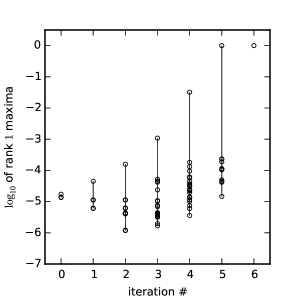
Figure 3.1. Comparing the maximum absolute values of entries from rank one terms of a CTD. After $6$ iterations Algorithm 2 converges to a rank $1$ tensor.

Another interesting case occurs when a tensor has multiple maximum entry candidates, either close to or exactly the same in magnitude. To explore this case, we construct an experiment similar to the previous one, namely, find the maximum absolute value of a CTD of dimension $d=6$ and $M=32$ samples in each direction. This CTD is constructed with the same rank $3$ random CTD as above, but this time we added in two spikes at random locations so that there are two maximal spikes of absolute value $3.5$. In cases such as this, Algorithm 2 can be run for a predetermined number of iterations, after which the factors are examined and a subset of candidates can be identified and explicitly verified. For example, in Figure 3.2, we observe that by iteration $6$ there are only two candidates for the location of the maximum. As a warning we note that allowing the code to continue to run many more iterations will leave only one term due to the finite reduction tolerance $\epsilon$ of $\tau_{\epsilon}$ in Algorithm 2. Indeed, in Figure 3.2 we observe the maximum entries of the two rank one terms begin to split around iteration number $26$, and by iteration $37$ only one term remains. This example illustrates a potential danger of insisting on a single term termination condition.

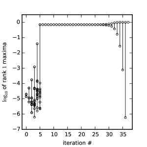
Figure 3.2. In this example there are two maxima of the same size. The values at these locations converge to $1/\sqrt{2}$ and the rest of the entries converge to $0$. If allowed to run long enough, the value at one of the locations becomes dominant due to the truncation error of the rank reduction algorithm. The other location is then eliminated by the algorithm and only one term remains.

4. CTD-based global optimization of multivariate functions

We describe an approach using Algorithm 2 for the global optimization of functions that admit low rank separated representations. We consider two types of problems: first, where the objective function is already in a separated form, ready to yield a CTD appropriate for use with Algorithm 2. The second, more general problem, is to construct a separated representation given data or an analytic expression of the function, from which a CTD can then be built.

In the first problem the objective function is already represented in separated form as in (2.1), and an interpolation scheme is associated with each direction. Such problems have been subject to growing interest due to the use of CTDs for solving operator equations, e.g., deterministic or stochastic PDE/ODE systems (see, for example, [5, 6, 13, 24, 11, 12]).

In the second problem the goal is to optimize a multivariate function where no separated representation is readily available. What typically is available is a data set of function values (scattered or on a grid). In such cases our recourse is to first construct a separated representation of the underlying multivariate objective function and then re-sample it in order to obtain a CTD of the form (2.2). The construction of a separated representation given a set of function values can be thought of as a regression problem, see [4, 15]. The algorithms in these papers use function samples to build a separated representation of form (2.1). Following [4], an interpolation scheme is set up in each direction and the ALS algorithm is used to reduce the problem to regression in a single variable. The univariate interpolation scheme may use a variety of possible bases, as well as nonlinear approximation techniques. Once a separated representation is constructed, the CTD for finding the global maxima is then obtained to satisfy the local interpolation requirement stated below. The resulting CTD is then used as input into Algorithm 2 to produce an approximation of the global maxima.

If the objective function is given analytically, it is preferable to use analytic techniques to approximate the original function via a separated representation. An example of this approach is included in Section 5.2 below.

We note that sampling becomes an important issue when finding global maxima of a function via Algorithm 2. The key sampling requirement is to ensure that the objective function can be interpolated at an arbitrary point from its sampled values up to a desired accuracy. This implies that sampling rate must depend on the local behavior of the function, e.g., the sampling rate is greater near singularities. For example, if a function has algebraic singularities, an efficient method to interpolate is to use wavelet bases. In such a case we emphasize the importance of using interpolating scaling functions, i.e., scaling functions whose coefficients are function values or are simply related to those. Since the global maxima are typically searched for in finite domains, the multiresolution basis should also work well in an interval (or a box in higher dimensions). This leads us to suggest the use of Lagrange interpolating polynomials within an adaptive spatial subdivision framework. We note that rescaled Lagrange interpolating polynomials form an orthonormal basis on an interval and the spatial subdivision is available as multiwavelet bases (see e.g., [1, 2]).

Finding the maximum entries of a CTD yields only an approximation of the maxima and their locations for the function. However, due to the interpolation requirements stated above these are high-quality approximations so that, if needed, a local optimization algorithm can then be used to find the true global maxima. Since in this case we use local optimization, it is preferable to oversample the CTD representation of a function, i.e. to use large $M_{j}$’s in (2.2). This will not result in a prohibitive cost as the rank reduction algorithms, e.g. ALS, that operate on CTDs scale linearly with respect to the number of samples in each direction [6]. However, the total number of samples needed to satisfy the local interpolation requirement may be large and, thus, additional steps to accelerate the reduction algorithm $\tau_{\epsilon}$ in Algorithm 2 may be required. One such technique consists of using the $QR$ factorization as explained in [8, Section 2.4].

5. Numerical examples

5.1. Comparison with power method algorithm from Section 2.2

To test Algorithm 2, we construct tensors from random factors and find the entries with the largest absolute value. For these examples we select dimension $d=8$ and set $M=32$ samples in each direction. The test CTDs are constructed by adding rank four and rank one CTDs together. The rank four CTDs are composed of random factors (vectors $\mathbf{u}_{j}^{(l)}$ in (2.2)) whose entries are drawn from the uniform distribution on $\left[.9,1\right]$ and the corresponding $s$-values are set to $1$. The rank one CTDs contain all zeros except for a magnitude $4$ spike added in at a random location. The CTDs in these examples have a unique maximum entry, and we chose to terminate the algorithm when the output CTD reaches separation rank one. We run tests for both Algorithm 2 and Algorithm 1, using for the rank reduction operation $\tau_{\epsilon}$ the CTD-ID algorithm with accuracy threshold $\epsilon=10^{-6}$ in the $s$-norm.

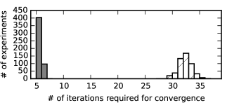
Figure 5.1. Histograms illustrating the number of iterations required for convergence to a rank one CTD by the power method optimization (hatched pattern) and the squaring method optimization (solid gray).

A histogram displaying the required number of iterations to converge for $500$ individual tests is shown in Figure 5.1. While both algorithms find the correct maximum location in all tests, Algorithm 2 outperforms Algorithm 1 in terms of the number of iterations required. While Algorithm 2 requires much fewer iterations than the power method for the same problem, a lingering concern may be that the squaring process in Algorithm 2 requires the reduction of CTDs with much larger separation ranks. In Figure 5.2 we show histograms of computation times. We observe that despite reducing larger separation rank CTDs, the computation times using Algorithm 2 are significantly smaller. These computation times are for our MATLAB code running on individual cores of a Intel Xeon $2.40$ GHz processor.

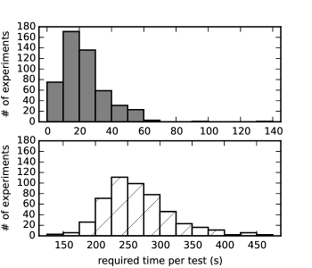
Figure 5.2. Histograms illustrating the computation times, in seconds, required for convergence to a rank one CTD by the power method optimization (hatched pattern) and the squaring method optimization (solid gray).

5.2. Optimization example

We reiterate that separated representations of general functions can be obtained numerically using only function evaluations, as described in [4, 15]. Once such a representation is obtained, an appropriate sampling yields a tensor in CTD format. In some cases, as in this example, this can be accomplished analytically.

As an example of constructing separated representations for optimization, we consider Ackley’s test function [3], commonly used for testing global optimization algorithms,

(5.1) $$u\left(\mathbf{x}\right)=a\,e^{-b\left(\frac{1}{d}\sum_{i=1}^{d}x_{i}^{2}\right)^{1/2}}+e^{\frac{1}{d}\sum_{i=1}^{d}\cos\left(cx_{i}\right)},$$

where $d$ is the number of dimensions and $a$, $b$, and $c$ are parameters. For our tests we set $d=10$, $a=20$, $b=0.2$, and $c=2\pi$. We choose this test function for two reasons: first, it has many local maxima, thus a local method without a good initial guess may not find the correct maximum. Second, one of the terms is not in separated form, hence we must construct a separated approximation of the function first.

The true maximum of (5.1) occurs at $\mathbf{x}=\mathbf{0}$ with a value of $u\left(\mathbf{0}\right)=a+e$. The first term in (5.1) is radially symmetric which we approximate with a linear combination of Gaussians using the approximation of $e^{-xy}$ from [7, Section 2.2],

(5.2) $$G_{e}\left(x\right)=\frac{hb}{2\sqrt{\pi d}}\sum_{j=0}^{R}\exp\left(-\frac{b^{2}}{4d}e^{s_{j}}-x^{2}e^{s_{j}}+\frac{1}{2}s_{j}\right),$$

where $s_{j}=s_{start}+jh$, and $h,\,\,s_{start},$ and $R$ are parameters chosen such that given $\epsilon,\delta>0$,

(5.3) $$\left|G_{e}\left(x\right)-e^{-\frac{b}{\sqrt{d}}x}\right|\leq\epsilon$$

for $0<\delta<x<\infty$. We arrive at the approximation of the first term in (5.1),

(5.4) $$\left|e^{-b\left(\frac{1}{d}\sum_{i=1}^{d}x_{i}^{2}\right)^{1/2}}-\sum_{j=0}^{R}w_{j}\prod_{i=1}^{d}\exp\left(-x_{i}^{2}e^{s_{j}}\right)\right|\leq\epsilon$$

where $w_{j}=\frac{hb}{2\sqrt{\pi d}}\exp\left(-\frac{b^{2}}{4d}e^{s_{j}}+\frac{1}{2}s_{j}\right)$.

To correctly sample (5.1), we first consider two terms of the function separately, the radially-symmetric exponential term, and the exponential cosine term which is already in separated form, $\exp\left(\frac{1}{d}\sum_{i=1}^{d}\cos\left(cx_{i}\right)\right)=\prod_{i=1}^{d}\exp\left(\frac{1}{d}\cos\left(cx_{i}\right)\right)$. These terms require different sampling strategies. The sampling rate of the radially-symmetric exponential term near the origin should be significantly higher than away from it. On the other hand, uniform sampling is sufficient for the exponential cosine term. We briefly discuss the combined sampling of these terms to satisfy both requirements.

To sample the radially-symmetric exponential term in (5.1), we use the expansion by Gaussians (5.2) as a guide. We choose $10$ equally-spaced points centered at zero and sample the Gaussian $e^{-x^{2}}$. For each Gaussian in (5.2), we scale these points by the factor $e^{s_{j}/2}$ in order to consistently sample each Gaussian independent of its scale. Since (5.2) includes a large number of rapidly decaying Gaussians, too many of the resulting samples will concentrate near the origin. Therefore, we select a subset as follows: first, we keep all samples from the sharpest Gaussian, $x_{0l}$, $l=1,\dots,10$. We then take the samples from second sharpest Gaussian and keep only those outside the range the previous samples, i.e., we keep $x_{1m}$ such that $\left|x_{1m}\right|>\max_{l}\left|x_{0l}\right|$, $m=1,\dots,10$. Repeating this process for all terms $j=0,1,\dots,R$ in expansion (5.2) yields samples for the radially-symmetric exponential term in (5.1).

We oversample the exponential cosine term using $16$ samples per oscillation. Notice that this sampling strategy is not sufficient for the radially-symmetric exponential term in (5.1) (and vice-versa). To combine these samples, we first find the radius where the sampling rate of the radially-symmetric exponential term in (5.1) drops below the sampling rate chosen to sample the exponential cosine term. We then remove all samples whose coordinates are greater in absolute value than the radius, and replace them with samples at the chosen rate of $16$ samples per oscillation. The resulting set of samples consists of $M=1080$ points for each direction $j=1,\dots,10$.

Using expansion (5.2) leads to a $77$ term CTD representation for the chosen accuracy $\epsilon=10^{-8}$ and parameter $\delta=3\cdot 10^{-6}$ in (5.3). An initial reduction of this CTD using the CTD-ID algorithm with accuracy threshold $\epsilon=10^{-6}$ in the Frobenius norm produces a CTD with separation rank $11$ representing the function $u\left(\mathbf{x}\right)$. We use this CTD as an input into Algorithm 2, yielding a rank one solution after $24$ iterations. We set the reduction tolerance in Algorithm 2 for this experiment to $\epsilon=10^{-6}$ and find the maximum entry of the tensor located at a distance $2.13\times 10^{-3}$ away from the function’s true maximum location, the origin. Using the output as the initial guess in a local, gradient-free, optimization algorithm (in our case a compass search, see e.g. [21]) yields the maximum value with relative error of $1.03\times 10^{-7}$ located at a distance $1.84\times 10^{-6}$ away from the origin.

6. Discussion and conclusions

Entries of a tensor in CTD format with the largest absolute value can be reliably identified by the new quadratically convergent algorithm, Algorithm 2. This algorithm, in turn, can be used for global optimization of multivariate functions that admit separated representations. Unlike algorithms based on random search strategies (see e.g. [19]), our approach allows the user to estimate the potential error of the result. The computational cost of Algorithm 2 is dominated by the cost of reducing the separation ranks of intermediate CTDs, not the dimension of the optimization problem. If ALS is used to reduce the separation rank and $d$ is the dimension, $r$ is the maximum separation rank (after reductions) during the iteration, and $M$ is the maximum number of components in each direction, then the computational cost of each rank reduction step can be estimated as $\mathcal{O}\left(r^{4}\cdot M\cdot d\cdot N_{iter}\right)$, where $N_{iter}$ is the number of iterations required by the ALS algorithm to converge. The computational cost of the CTD-ID algorithm is estimated as $\mathcal{O}\left(r^{3}\cdot M\cdot d\right)$ and, if it is used instead of ALS, the reduction step is faster by a factor of $\mathcal{O}\left(r\cdot N_{iter}\right)$ [8]. We note that, while linear in dimension, Algorithm 2 may require significant computational resources due to the cubic (or quartic for ALS) dependence on the separation rank $r$.

Finally, we note that the applicability of our approach to global optimization extends beyond the use of separated representations of multivariate functions or tensors in CTD format. In fact, any structural representation of a multivariate function that allows rapid computation of the Hadamard product of corresponding tensors and has an associated algorithm for reducing the complexity of the representation should work in a manner similar to Algorithm 2.

References

- [1] B. Alpert. A class of bases in for the sparse representation of integral operators. SIAM J. Math. Anal, 24(1):246–262, 1993.
- [2] B. Alpert, G. Beylkin, D. Gines, and L. Vozovoi. Adaptive solution of partial differential equations in multiwavelet bases. J. Comput. Phys., 182(1):149–190, 2002.
- [3] T. Bäck. Evolutionary algorithms in theory and practice: evolution strategies, evolutionary programming, genetic algorithms. Oxford University Press, 1996.
- [4] G. Beylkin, J. Garcke, and M. J. Mohlenkamp. Multivariate regression and machine learning with sums of separable functions. SIAM Journal on Scientific Computing, 31(3):1840–1857, 2009.
- [5] G. Beylkin and M. J. Mohlenkamp. Numerical operator calculus in higher dimensions. Proc. Natl. Acad. Sci. USA, 99(16):10246–10251, August 2002.
- [6] G. Beylkin and M. J. Mohlenkamp. Algorithms for numerical analysis in high dimensions. SIAM J. Sci. Comput., 26(6):2133–2159, July 2005.
- [7] G. Beylkin and L. Monzón. Approximation of functions by exponential sums revisited. Appl. Comput. Harmon. Anal., 28(2):131–149, 2010.
- [8] D. J. Biagioni, D. Beylkin, and G. Beylkin. Randomized interpolative decomposition of separated representations. Journal of Computational Physics, 281:116–134, 2015.
- [9] R. Bro. Parafac. Tutorial & Applications. In Chemom. Intell. Lab. Syst., Special Issue 2nd Internet Conf. in Chemometrics (incinc’96), volume 38, pages 149–171, 1997. http://www.models.kvl.dk/users/rasmus/presentations/parafac_tutorial/paraf.htm.
- [10] J. D. Carroll and J. J. Chang. Analysis of individual differences in multidimensional scaling via an N-way generalization of Eckart-Young decomposition. Psychometrika, 35:283–320, 1970.
- [11] F. Chinesta, P. Ladeveze, and E. Cueto. A short review on model order reduction based on proper generalized decomposition. Archives of Computational Methods in Engineering, 18(4):395–404, 2011.
- [12] H. Cho, D. Venturi, and G.E. Karniadakis. Numerical methods for high-dimensional probability density function equations. Journal of Computational Physics, 305:817–837, 2016.
- [13] A. Doostan and G. Iaccarino. A least-squares approximation of partial differential equations with high-dimensional random inputs. Journal of Computational Physics, 228(12):4332–4345, 2009.
- [14] A. Doostan, G. Iaccarino, and N. Etemadi. A least-squares approximation of high-dimensional uncertain systems. Technical Report Annual Research Brief, Center for Turbulence Research, Stanford University, 2007.
- [15] A. Doostan, A. Validi, and G. Iaccarino. Non-intrusive low-rank separated approximation of high-dimensional stochastic models. Comput. Methods Appl. Mech. Engrg., 263:42–55, 2013.
- [16] M. Espig, W. Hackbusch, A. Litvinenko, H.G. Matthies, and E. Zander. Efficient analysis of high dimensional data in tensor formats. In Sparse Grids and Applications, pages 31–56. Springer, 2013.
- [17] M. Hadigol, A. Doostan, H. Matthies, and R. Niekamp. Partitioned treatment of uncertainty in coupled domain problems: A separated representation approach. Computer Methods in Applied Mechanics and Engineering, 274:103–124, 2014.
- [18] R. A. Harshman. Foundations of the Parafac procedure: model and conditions for an “explanatory” multi-mode factor analysis. Working Papers in Phonetics 16, UCLA, 1970. http://publish.uwo.ca/harshman/wpppfac0.pdf.
- [19] R. Horst and P. M. Pardalos. Handbook of global optimization, volume 2. Springer Science & Business Media, 2013.
- [20] T. G. Kolda and B. W. Bader. Tensor decompositions and applications. SIAM Review, 51(3):455–500, 2009.
- [21] T. G. Kolda, R.M. Lewis, and V. Torczon. Optimization by direct search: New perspectives on some classical and modern methods. SIAM review, 45(3):385–482, 2003.
- [22] A. Nouy. A generalized spectral decomposition technique to solve a class of linear stochastic partial differential equations. Computer Methods in Applied Mechanics and Engineering, 196(37-40):4521–4537, 2007.
- [23] A. Nouy. Generalized spectral decomposition method for solving stochastic finite element equations: Invariant subspace problem and dedicated algorithms. Computer Methods in Applied Mechanics and Engineering, 197:4718–4736, 2008.
- [24] A. Nouy. Proper generalized decompositions and separated representations for the numerical solution of high dimensional stochastic problems. Archives of Computational Methods in Engineering, 17:403–434, 2010.
- [25] J.C. Spall. Introduction to stochastic search and optimization: estimation, simulation, and control, volume 65. John Wiley & Sons, 2005.
- [26] G. Tomasi and R. Bro. A comparison of algorithms for fitting the PARAFAC model. Comput. Statist. Data Anal., 50(7):1700–1734, 2006.