Efficient Nonparametric Smoothness Estimation

Abstract

Sobolev quantities (norms, inner products, and distances) of probability density functions are important in the theory of nonparametric statistics, but have rarely been used in practice, partly due to a lack of practical estimators. They also include, as special cases, $L^{2}$ quantities which are used in many applications. We propose and analyze a family of estimators for Sobolev quantities of unknown probability density functions. We bound the bias and variance of our estimators over finite samples, finding that they are generally minimax rate-optimal. Our estimators are significantly more computationally tractable than previous estimators, and exhibit a statistical/computational trade-off allowing them to adapt to computational constraints. We also draw theoretical connections to recent work on fast two-sample testing. Finally, we empirically validate our estimators on synthetic data.

1 Introduction

$L^{2}$ quantities (i.e., inner products, norms, and distances) of continuous probability density functions are important information theoretic quantities with many applications in machine learning and signal processing. For example, estimates of the $L^{2}$ norm as can be used for goodness-of-fit testing Goria et al. (2005), image registration and texture classification (Hero et al., 2002), and parameter estimation in semi-parametric models Wolsztynski et al. (2005). $L^{2}$ inner products estimates can be used with linear or polynomial kernels to generalize kernel methods to inputs which are distributions rather than numerical vectors. (Póczos et al., 2012b) Estimators of $L^{2}$ distance have been used for two-sample testing (Anderson et al., 1994; Pardo, 2005), transduction learning (Quadrianto et al., 2009), and machine learning on distributional inputs (Póczos et al., 2012a). Principe (2010) gives further applications of $L^{2}$ quantities to adaptive information filtering, classification, and clustering.

$L^{2}$ quantities are a special case of less-well-known Sobolev quantities. Sobolev norms measure global smoothness of a function in terms of integrals of squared derivatives. For example, for a non-negative integer $s$ and a function $f:\mathbb{R}\to\mathbb{R}$ with an $s^{th}$ derivative $f^{(s)}$, the $s$-order Sobolev norm $\|\cdot\|_{H^{s}}$ is given by $\|f\|_{H^{s}}=\int_{\mathbb{R}}\left(f^{(s)}(x)\right)^{2}\,dx$ (when this quantity is finite). See Section 2 for more general definitions, and see Leoni (2009) for an introduction to Sobolev spaces.

Estimation of general Sobolev norms has a long history in nonparametric statistics (e.g., Schweder (1975); Ibragimov and Khasminskii (1978); Hall and Marron (1987); Bickel and Ritov (1988)) This line of work was motivated by the role of Sobolev norms in many semi- and non-parametric problems, including density estimation, density functional estimation, and regression, (see Tsybakov (2008), Section 1.7.1) where they dictate the convergence rates of estimators. Despite this, to our knowledge, these quantities have never been studied in real data, leaving an important gap between the theory and practice of nonparametric statistics. We suggest this is in part due a lack of practical estimators for these quantities. For example, the only one of the above estimators that is statistically minimax-optimal (Bickel and Ritov, 1988) is extremely difficult to compute in practice, requiring numerical integration over each of $O(n^{2})$ different kernel density estimates, where $n$ denotes the sample size. We know of no estimators previously proposed for Sobolev inner products and distances.

The main goal of this paper is to propose and analyze a family of computationally and statistically efficient estimators for Sobolev inner products, norms, and distances. Our specific contributions are:

1. We propose a family of nonparametric estimators for Sobolev norms, inner products, and distances (Section 4).

2. We analyze the bias and variance of the estimators. Assuming the underlying density functions have bounded support in $\mathbb{R}^{D}$ and lie in a Sobolev class of sufficient smoothness parametrized by $s^{\prime}$, we show that the estimator for Sobolev quantities of order $s<s^{\prime}$ converges to the true value at the “parametric” rate of $O(n^{-1})$ in mean squared error when $s^{\prime}\geq 2s+D/4$, and at a slower rate of $O\left(n^{\frac{8(s-s^{\prime})}{4s^{\prime}+D}}\right)$ otherwise. (Section 5).

3. We derive asymptotic distributions for our estimators, and we use these to derive tests for the general statistical problem of two-sample testing. We also draw theoretical connections between our test and the recent work on nonparametric two-sample testing. (Section 9).

4. We validate our theoretical results on simulated data. (Section 8).

In terms of mean squared error, minimax lower bounds matching our convergence rates over Sobolev or Hölder smoothness classes have been shown by Krishnamurthy et al. (2014b) for $s=0$ (i.e., $L^{2}$ quantities), and Birgé and Massart (1995) for Sobolev norms with integer $s$. We conjecture but do not prove that our estimator is minimax rate-optimal for all Sobolev quantities and $s\in[0,\infty)$.

As described in Section 7, our estimators are computable in $O(n^{1+\varepsilon})$ time using only basic matrix operations, where $n$ is the sample size and $\varepsilon\in(0,1)$ is a tunable parameter trading statistical and computational efficiency; the smallest value of $\varepsilon$ at which the estimator continues to be minimax rate-optimal approaches $0$ as we assume more smoothness of the true density.

2 Problem setup and notation

Let $\mathcal{X}=[-\pi,\pi]^{D}$ and let $\mu$ denote the Lebesgue measure on $\mathcal{X}$. For $D$-tuples $z\in\mathbb{Z}^{D}$ of integers, let $\psi_{z}\in L^{2}=L^{2}(\mathcal{X})$ defined by $\psi_{z}(x)=e^{-i\langle z,x\rangle}$ for all $x\in\mathcal{X}$ denote the $z^{th}$ element of the $L^{2}$-orthonormal Fourier basis, and, for $f\in L^{2}$, let $\widetilde{f}(z):=\langle\psi_{z},f\rangle_{L^{2}}=\int_{\mathcal{X}}\psi_{z}(x)\overline{f(x)}\,d\mu(x)$ denote the $z^{th}$ Fourier coefficient of $f$. For any $s\in[0,\infty)$, define the Sobolev space $H^{s}=H^{s}(\mathcal{X})\subseteq L^{2}$ of order $s$ on $\mathcal{X}$ by

$$H^{s}=\left\{f\in L^{2}:\sum_{z\in\mathbb{Z}^{D}}z^{2s}\left|\widetilde{f}(z)\right|^{2}<\infty\right\}.$$ (1)

Fix a known $s\in[0,\infty)$ and a unknown probability density functions $p,q\in H^{s}$, and suppose we have $n$ IID samples $X_{1},...,X_{n}\sim p$ and $Y_{1},\dots,Y_{n}\sim q$ from each of $p$ and $q$. We are interested in estimating the inner product

$$\langle p,q\rangle_{H^{s}}:=\sum_{z\in\mathbb{Z}^{D}}z^{2s}\widetilde{p}(z)\overline{\widetilde{q}(z)}\quad\mbox{ defined for all }\quad p,q\in H^{s}.$$ (2)

Estimating the inner product gives an estimate for the (squared) induced norm and distance, since

$$\|p\|_{H^{s}}^{2}:=\sum_{z\in\mathbb{Z}^{D}}z^{2s}\left|\widetilde{p}(z)\right|^{2}=\langle p,p\rangle_{H^{s}}\quad\mbox{ and }\quad\|p-q\|_{H^{s}}^{2}=\|p\|_{H^{s}}^{2}-2\langle p,q\rangle_{H^{s}}+\|q\|_{H^{s}}^{2}.$$ (3)

Since our theoretical results assume the samples from $p$ and $q$ are independent, when estimating $\|p\|_{H^{s}}^{2}$, we split the sample from $p$ in half to compute two independent estimates of $\widetilde{p}$, although this may not be optimal in practice.

For a more classical intuition, we note that, in the case $D=1$ and $s\in\{0,1,2,\dots\}$, (via Parseval’s identity and the identity $\widetilde{f^{(s)}}(z)=(iz)^{s}\widetilde{f}(z)$), that one can show the following: $H^{s}$ includes the subspace of $L^{2}$ functions with at least $s$ derivatives in $L^{2}$ and, if $f^{(s)}$ denotes the $s^{th}$ derivative of $f$

$$\|f\|_{H^{s}}^{2}=2\pi\int_{\mathcal{X}}\left(f^{(s)}(x)\right)^{2}\,dx=2\pi\left\|f^{(s)}\right\|_{L^{2}}^{2},\quad\forall f\in H^{s}.$$ (4)

In particular, when $s=0$, $H^{s}=L^{2}$, $\|\cdot\|_{H^{s}}=\|\cdot\|_{L^{2}}$, and $\langle\cdot,\cdot\rangle_{H^{s}}=\langle\cdot,\cdot\rangle_{L^{2}}$. As we describe in the supplement, equation (4) and our results generalizes trivially to weak derivatives, as well as to non-integer $s\in[0,\infty)$ via a notion of fractional derivative.

2.1 Unbounded domains

A notable restriction above is that $p$ and $q$ are supported in $\mathcal{X}:=[-\pi,\pi]^{D}$. In fact, our estimators and tests are well-defined and valid for densities supported on arbitrary subsets of $\mathbb{R}^{D}$. In this case, they act on the $2\pi$-periodic summation $p_{2\pi}:[-\pi,\pi]^{D}\to[0,\infty]$ defined for $x\in\mathcal{X}$ by $p_{2\pi}(x):=\sum_{z\in\mathbb{Z}^{D}}p(x+2\pi z)$, which is itself a probability density function on $\mathcal{X}$. For example, the estimator for $\|p\|_{H^{s}}$ will instead estimate $\|p_{2\pi}\|_{H^{s}}$, and the two-sample test for distributions $p$ and $q$ will attempt to distinguish $p_{2\pi}$ from $q_{2\pi}$. In most cases, this is not problematic; for example, for most realistic probability densities, $p$ and $p_{2\pi}$ have similar orders of smoothness, and $p_{2\pi}=q_{2\pi}$ if and only if $p=q$. However, there are (meagre) sets of exceptions; for example, if $q$ is a translation of $p$ by exactly $2\pi$, then $p_{2\pi}=q_{2\pi}$, and one can craft a highly discontinuous function $p$ such that $p_{2\pi}$ is uniform on $\mathcal{X}$. (Zygmund, 2002) These exceptions make it difficult to extend theoretical results to densities with arbitrary support, but in practice, they are fixed simply by randomly rescaling the data (similar to the approach of Chwialkowski et al. (2015)). If the densities have (known) bounded support, they can simply be shifted and scaled to be supported on $\mathcal{X}$.

3 Related work

There is a large body of work on estimating nonlinear functionals of probability densities, with various generalizations in terms of the class of functionals considered. Table 1 gives a subset of such work, for functionals related to Sobolev quantities. As shown in Section 2, the functional form we consider is a strict generalization of $L^{2}$ norms, Sobolev norms, and $L^{2}$ inner products. It overlaps with, but is neither a special case nor a generalization of the remaining functional forms in the table.

Functional Name	Functional Form	References
$L^{2}$ norms	$\|p\|_{L^{2}}^{2}=\int\left(p(x)\right)^{2}\,dx$	Schweder (1975); Giné and Nickl (2008)
(Integer) Sobolev norms	$\|p\|_{H^{k}}^{2}=\int\left(p^{(k)}(x)\right)^{2}\,dx$	Bickel and Ritov (1988)
Density functionals	$\int\varphi(x,p(x))\,dx$	Laurent (1992); Laurent et al. (1996)
Derivative functionals	$\int\varphi(x,p(x),p^{\prime}(x),\dots,p^{(k)}(x))\,dx$	Birgé and Massart (1995)
$L^{2}$ inner products	$\langle p_{1},p_{2}\rangle_{L^{2}}=\int p_{1}(x)p_{2}(x)\,dx$	Krishnamurthy et al. (2014b, a)
Multivariate functionals	$\int\varphi(x,p_{1}(x),\dots,p_{k}(x))\,dx$	Singh and Póczos (2014b); Kandasamy et al. (2015)

Table 1: Some related functional forms for which estimators for which nonparametric estimators have been developed and analyzed. $p,p_{1},...,p_{k}$ are unknown probability densities, from each of which we draw $n$ IID samples, $\varphi$ is a known real-valued measurable function, and $k$ is a non-negative integer.

Nearly all of the above approaches compute an optimally smoothed kernel density estimate and then perform bias corrections based on Taylor series expansions of the functional of interest. They typically consider distributions with densities that are $\beta$-Hölder continuous and satisfy periodicity assumptions of order $\beta$ on the boundary of their support, for some constant $\beta>0$ (see, for example, Section 4 of Krishnamurthy et al. (2014b) for details of these assumptions). The Sobolev class we consider is a strict superset of this Hölder class, permitting, for example, certain “small” discontinuities. In this regard, our results are slightly more general than most of these prior works.

Finally, there is much recent work on estimating entropies, divergences, and mutual informations, using methods based on kernel density estimates (Singh and Póczos, 2014a, b; Moon et al., 2016; Krishnamurthy et al., 2014b, a; Kandasamy et al., 2015) or $k$-nearest neighbor statistics (Leonenko et al., 2008; Póczos and Schneider, 2011; Moon and Hero, 2014b, a). In contrast, our estimators are more similar to orthogonal series density estimators, which are computationally attractive because they require no pairwise operations between samples. However, they require quite different theoretical analysis; unlike prior work, our estimator is constructed and analyzed entirely in the frequency domain, and then related to the data domain via Parseval’s identity. We hope our analysis can be adapted to analyze new, computationally efficient information theoretic estimators.

4 Motivation and construction of our estimator

For a non-negative integer parameter $Z_{n}$ (to be specified later), let

$$p_{n}:=\sum_{\|z\|_{\infty}\leq Z_{n}}\widetilde{p}(z)\psi_{z}\quad\mbox{ and }\quad q_{n}:=\sum_{\|z\|_{\infty}\leq Z_{n}}\widetilde{q}(z)\psi_{z}\quad\mbox{ where }\quad\|z\|_{\infty}:=\max_{j\in\{1,\dots,D\}}z_{j}$$ (5)

denote the $L^{2}$ projections of $p$ and $q$, respectively, onto the linear subspace spanned by the $L^{2}$-orthonormal family $\mathcal{F}_{n}:=\{\psi_{z}:z\in\mathbb{Z}^{D},|z|\leq Z_{n}\}$. Note that, since $\widetilde{\psi_{z}}(y)=0$ whenever $y\neq z$, the Fourier basis has the special property that it is orthogonal in $\langle\cdot,\cdot\rangle_{H^{s}}$ as well. Hence, since $p_{n}$ and $q_{n}$ lie in the span of $\mathcal{F}_{n}$ while $p-p_{n}$ and $q-q_{n}$ lie in the span of $\{\psi_{z}:z\in\mathbb{Z}\}\backslash\mathcal{F}_{n}$, $\langle p-p_{n},q_{n}\rangle_{H^{s}}=\langle p_{n},q-q_{n}\rangle_{H^{s}}=0$. Therefore,

$$\langle p,q\rangle_{H^{s}} =\langle p_{n},q_{n}\rangle_{H^{s}}+\langle p-p_{n},q_{n}\rangle_{H^{s}}+\langle p_{n},q-q_{n}\rangle_{H^{s}}+\langle p-p_{n},q-q_{n}\rangle_{H^{s}}$$

$$=\langle p_{n},q_{n}\rangle_{H^{s}}+\langle p-p_{n},q-q_{n}\rangle_{H^{s}}.$$ (6)

We propose an unbiased estimate of $S_{n}:=\langle p_{n},q_{n}\rangle_{H^{s}}=\sum_{\|z\|_{\infty}\leq Z_{n}}z^{2s}\widetilde{p}_{n}(z)\overline{\widetilde{q}_{n}(z)}$. Notice that Fourier coefficients of $p$ are the expectations $\widetilde{p}(z)=\mathop{\mathbb{E}}_{X\sim p}\left[\psi_{z}(X)\right]$. Thus, $\hat{p}(z):=\frac{1}{n}\sum_{j=1}^{n}\psi_{z}(X_{j})$ and $\hat{q}(z):=\frac{1}{n}\sum_{j=1}^{n}\psi_{z}(Y_{j})$ are independent unbiased estimates of $\widetilde{p}$ and $\widetilde{q}$, respectively. Since $S_{n}$ is bilinear in $\widetilde{p}$ and $\widetilde{q}$, the plug-in estimator for $S_{n}$ is unbiased. That is, our estimator for $\langle p,q\rangle_{H^{s}}$ is

$$\hat{S}_{n}:=\sum_{\|z\|_{\infty}\leq Z_{n}}z^{2s}\hat{p}(z)\overline{\hat{q}(z)}.$$ (7)

5 Finite sample bounds

Here, we present our main theoretical results, bounding the bias, variance, and mean squared error of our estimator for finite $n$.

By construction, our estimator satisfies

$$\mathop{\mathbb{E}}\left[\hat{S}_{n}\right]=\sum_{\|z\|_{\infty}\leq Z_{n}}z^{2s}\mathop{\mathbb{E}}\left[\hat{p}(z)\right]\overline{\mathop{\mathbb{E}}\left[\hat{q}(z)\right]}=\sum_{\|z\|_{\infty}\leq Z_{n}}z^{2s}\widetilde{p}_{n}(z)\overline{\widetilde{q}_{n}(z)}=S_{n}.$$

Thus, via (6) and Cauchy-Schwarz, the bias of the estimator $\hat{S}_{n}$ satisfies

$$\left|\mathop{\mathbb{E}}\left[\hat{S}_{n}\right]-\langle p,q\rangle_{H^{s}}\right|=\left|\langle p-p_{n},q-q_{n}\rangle_{H^{s}}\right|\leq\sqrt{\left\|p-p_{n}\right\|_{H^{s}}^{2}\left\|q-q_{n}\right\|_{H^{s}}^{2}}.$$ (8)

$\left\|p-p_{n}\right\|_{H^{s}}$ is the error of approximating $p$ by an order-$Z_{n}$ trigonometric polynomial, a classic problem in approximation theory, for which Theorem 2.2 of Kreiss and Oliger (1979) shows:

$$\mbox{ if }p\in H^{s^{\prime}}\mbox{ for some }s^{\prime}>s,\quad\mbox{ then }\quad\left\|p-p_{n}\right\|_{H^{s}}\leq\|p\|_{H^{s^{\prime}}}Z_{n}^{s-s^{\prime}}.$$ (9)

In combination with (8), this implies the following bound on the bias of our estimator:

Theorem 1.

(Bias bound) If $p,q\in H^{s^{\prime}}$ for some $s^{\prime}>s$, then, for $C_{B}:=\|p\|_{H^{s^{\prime}}}\|q\|_{H^{s^{\prime}}}$,

$$\left|\mathop{\mathbb{E}}\left[\hat{S}_{n}\right]-\langle p,q\rangle_{H^{s}}\right|\leq C_{B}Z_{n}^{2(s-s^{\prime})}$$ (10)

Hence, the bias of $\hat{S}_{n}$ decays polynomially in $Z_{n}$, with a power depending on the “extra” $s^{\prime}-s$ orders of smoothness available. On the other hand, as we increase $Z_{n}$, the number of frequencies at which we estimate $\hat{p}$ increases, suggesting that the variance of the estimator will increase with $Z_{n}$. Indeed, this is expressed in the following bound on the variance of the estimator.

Theorem 2.

(Variance bound) If $p,q\in H^{s^{\prime}}$ for some $s^{\prime}\geq s$, then

$$\mathbb{V}\left[\hat{S}_{n}\right]\leq 2C_{1}\frac{Z_{n}^{4s+D}}{n^{2}}+\frac{C_{2}}{n},$$ (11)

where $C_{1}$ and $C_{2}$ are the constants (in $n$)

$$C_{1}:=\frac{2^{D}\Gamma(4s+1)}{\Gamma(4s+D+1)}\|p\|_{L^{2}}\|q\|_{L^{2}}$$ (12)

and $C_{2}:=\left(\|p\|_{H^{s}}+\|q\|_{H^{s}}\right)\|p\|_{W^{2s,4}}\|q\|_{W^{2s,4}}+\|p\|_{H^{s}}^{4}\|q\|_{H^{s}}^{4}$.

The proof of Theorem 2 is perhaps the most significant theoretical contribution of this work. Due to space constraints, the proof is given in the appendix. Combining Theorems 10 and 2 gives a bound on the mean squared error (MSE) of $\hat{S}_{n}$ via the usual decomposition into squared bias and variance:

Corollary 3.

(Mean squared error bound) If $p,q\in H^{s^{\prime}}$ for some $s^{\prime}>s$, then

$$\mathop{\mathbb{E}}\left[\left(\hat{S}_{n}-\langle p,q\rangle_{H^{s}}\right)^{2}\right]\leq C_{B}^{2}Z_{n}^{4(s-s^{\prime})}+2C_{1}\frac{Z_{n}^{4s+D}}{n^{2}}+\frac{C_{2}}{n}.$$ (13)

If, furthermore, we choose $Z_{n}\asymp n^{\frac{2}{4s^{\prime}+D}}$ (optimizing the rate in inequality 13), then

$$\mathop{\mathbb{E}}\left[\left(\hat{S}_{n}-\langle p,q\rangle_{H^{2}}\right)^{2}\right]\asymp n^{\max\left\{\frac{8(s-s^{\prime})}{4s^{\prime}+D},-1\right\}}.$$ (14)

Corollary 3 recovers the phenomenon discovered by Bickel and Ritov (1988): when $s^{\prime}\geq 2s+\frac{D}{4}$, the minimax optimal MSE decays at the “semi-parametric” $n^{-1}$ rate, whereas, when $s^{\prime}\in\left(s,2s+\frac{D}{4}\right)$, the MSE decays at a slower rate. Also, the estimator is $L^{2}$-consistent if $Z_{n}\to\infty$ and $Z_{n}n^{-\frac{2}{4s+D}}\to 0$ as $n\to\infty$. This is useful in practice, since $s$ is known but $s^{\prime}$ is not.

6 Asymptotic distributions

In this section, we derive the asymptotic distributions of our estimator in two cases: (1) the inner product estimator and (2) the distance estimator in the case $p=q$. These results provide confidence intervals and two-sample tests without computationally intensive resampling. While (1) is more general in that it can be used with (3) to bound the asymptotic distributions of the norm and distance estimators, (2) provides a more precise result leading to a more computationally and statistically efficient two-sample test. Proofs are given in the supplementary material.

Theorem 4 shows that our estimator has a normal asymptotic distribution, assuming $Z_{n}\to\infty$ slowly enough as $n\to\infty$, and also gives a consistent estimator for its asymptotic variance. From this, one can easily estimate asymptotic confidence intervals for inner products, and hence also for norms.

Theorem 4.

(Asymptotic normality) Suppose that, for some $s^{\prime}>2s+\frac{D}{4}$, $p,q\in H^{s^{\prime}}$, and suppose $Z_{n}n^{\frac{1}{4(s-s^{\prime})}}\to\infty$ and $Z_{n}n^{-\frac{1}{4s+D}}\to 0$ as $n\to\infty$. Then, $\hat{S}_{n}$ is asymptotically normal with mean $\langle p,q\rangle_{H^{s}}$. In particular, for $j\in\{1,\dots,n\}$ and $z\in\mathbb{Z}^{D}$ with $\|z\|_{\infty}\leq Z_{n}$, define $W_{j,z}:=z^{s}e^{izX_{j}}$ and $V_{j,z}:=z^{s}e^{izY_{j}}$, so that $W_{j}$ and $V_{j}$ are column vectors in $\mathbb{R}^{(2Z_{n})^{D}}$. Let $\overline{W}:=\frac{1}{n}\sum_{j=1}^{n}W_{j},\overline{V}:=\frac{1}{n}\sum_{j=1}^{n}V_{j}\in\mathbb{R}^{(2Z_{n})^{D}},$

$$\Sigma_{W}:=\frac{1}{n}\sum_{j=1}^{n}(W_{j}-\overline{W})(W_{j}-\overline{W})^{T},\quad\mbox{ and }\quad\Sigma_{V}:=\frac{1}{n}\sum_{j=1}^{n}(V_{j}-\overline{V})(V_{j}-\overline{V})^{T}\in\mathbb{R}^{(2Z_{n})^{D}\times(2Z_{n})^{D}}$$

denote the empirical means and covariances of $W$ and $V$, respectively. Then, for

$$\hat{\sigma}_{n}^{2}:=\begin{bmatrix}\overline{V}\\ \overline{W}\end{bmatrix}^{T}\begin{bmatrix}\Sigma_{W}&0\\ 0&\Sigma_{V}\end{bmatrix}\begin{bmatrix}\overline{V}\\ \overline{W}\end{bmatrix},\quad\mbox{ we have }\quad\sqrt{n}\left(\frac{\hat{S}_{n}-\langle p,q\rangle_{H^{s}}}{\hat{\sigma}_{n}}\right)\stackrel{{\scriptstyle D}}{{\to}}\mathcal{N}(0,1),$$

where $\stackrel{{\scriptstyle D}}{{\to}}$ denotes convergence in distribution.

Since distances can be written as a sum of three inner products (Eq. (3)), Theorem 4 might suggest an asymptotic normal distribution for Sobolev distances. However, extending asymptotic normality from inner products to their sum requires that the three estimates be independent, and hence that we split data between the three estimates. This is inefficient in practice and somewhat unnatural, as we know, for example, that distances should be non-negative. For the particular case $p=q$ (as in the null hypothesis of two-sample testing), the following theorem provides a more precise asymptotic ($\chi^{2}$) distribution of our Sobolev distance estimator, after an extra decorrelation step. This gives, for example, a more powerful two-sample test statistic (see Section 9 for details).

Theorem 5.

(Asymptotic null distribution) Suppose that, for some $s^{\prime}>2s+\frac{D}{4}$, $p,q\in H^{s^{\prime}}$, and suppose $Z_{n}n^{\frac{1}{4(s-s^{\prime})}}\to\infty$ and $Z_{n}n^{-\frac{1}{4s+D}}\to 0$ as $n\to\infty$. For $j\in\{1,\dots,n\}$ and $z\in\mathbb{Z}^{D}$ with $\|z\|_{\infty}\leq Z_{n}$, define $W_{j,z}:=z^{s}\left(e^{-izX_{j}}-e^{-izY_{j}}\right)$, so that $W_{j}$ is a column vector in $\mathbb{R}^{(2Z_{n})^{D}}$. Let

$$\overline{W}:=\frac{1}{n}\sum_{j=1}^{n}W_{j}\in\mathbb{R}^{(2Z_{n})^{D}}\quad\mbox{ and }\quad\Sigma:=\frac{1}{n}\sum_{j=1}^{n}\left(W_{j}-\overline{W}\right)\left(W_{j}-\overline{W}\right)^{T}\in\mathbb{R}^{(2Z_{n})^{D}\times(2Z_{n})^{D}}$$

denote the empirical mean and covariance of $W$, and define $T:=n\overline{W}^{T}\Sigma^{-1}\overline{W}$. Then, if $p=q$, then

$$Q_{\chi^{2}((2Z_{n})^{D})}(T)\stackrel{{\scriptstyle D}}{{\to}}\operatorname{Uniform}([0,1])\quad\mbox{ as }\quad n\to\infty,$$

where $Q_{\chi^{2}(d)}:[0,\infty)\to[0,1]$ denotes the quantile function (inverse CDF) of the $\chi^{2}$ distribution $\chi^{2}(d)$ with $d$ degrees of freedom.

Let $\hat{M}$ denote our estimator for $\|p-q\|_{H^{s}}$ (i.e., plugging $\hat{S}_{n}$ into (3)). While Theorem 5 immediately provides a valid two-sample test of desired level, it is not immediately clear how this relates to $\hat{M}$, nor is there any suggestion of why the test statistic ought to be a good (i.e., consistent) one. Some intuition is as follows. Notice that $\hat{M}=\overline{W}^{T}\overline{W}$. Since, by the central limit theorem, $\overline{W}$ has a normal asymptotic distribution, if the components of $\overline{W}$ were uncorrelated (and $Z_{n}$ were fixed), we would expect $n\hat{M}$ to have an asymptotic $\chi^{2}$ distribution with $(2Z_{n})^{D}$ degrees of freedom. However, because we use the same data to compute each component of $\hat{M}$, they are not typically uncorrelated, and so the asymptotic distribution of $\hat{M}$ is difficult to derive. This motivates the statistic $T=\left(\sqrt{\Sigma_{W}^{-1}}\overline{W}\right)^{T}\sqrt{\Sigma_{W}^{-1}}\overline{W}$, since the components of $\sqrt{\Sigma_{W}^{-1}}\overline{W}$ are (asymptotically) uncorrelated.

7 Parameter selection and statistical/computational trade-off

Here, we give statistical and computational considerations for choosing the smoothing parameter $Z_{n}$.

Statistical perspective: In practice, of course, we do not typically know $s^{\prime}$, so we cannot simply set $Z_{n}\asymp n^{\frac{2}{4s^{\prime}+D}}$, as suggested by the mean squared error bound (14). Fortunately (at least for ease of parameter selection), when $s^{\prime}\geq 2s+\frac{D}{4}$, the dominant term of (14) is $C_{2}/n$ for $Z_{n}\asymp n^{-\frac{1}{4s+D}}$. Hence if we are willing to assume that the density has at least $2s+\frac{D}{4}$ orders of smoothness (which may be a mild assumption in practice), then we achieve statistical optimality (in rate) by setting $Z_{n}\asymp n^{-\frac{1}{4s+D}}$, which depends only on known parameters. On the other hand, the estimator can continue to benefit from additional smoothness computationally.

Computational perspective One attractive property of the estimator discussed is its computational simplicity and efficiency with respect to $n$, in low dimensions. Most competing nonparametric estimators, such as kernel-based or nearest-neighbor methods, either take $O(n^{2})$ time or rely on complex data structures such as $k$-d trees or cover trees (Ram et al., 2009) for $O(2^{D}n\log n)$ time performance. Since computing the estimator takes $O(nZ_{n}^{D})$ time and $O(Z_{n}^{D})$ memory (that is, the cost of estimating each of $(2Z_{n})^{D}$ Fourier coefficients by an average), a statistically optimal choice of $Z_{n}$ gives a runtime of $O\left(n^{\frac{4s^{\prime}+2D}{4s^{\prime}+D}}\right)$. Since the estimate requires only a vector outer product, exponentiation, and averaging, the constants involved are small and computations parallelize trivially over frequencies and data.

Under severe computational constraints, for very large data sets, or if $D$ is large relative to $s^{\prime}$, we can reduce $Z_{n}$ to trade off statistical for computational efficiency. For example, if we want an estimator with runtime $O(n^{1+\theta})$ and space requirement $O(n^{\theta})$ for some $\theta\in\left(0,\frac{2D}{4s^{\prime}+D}\right)$, setting $Z_{n}\asymp n^{\theta/D}$ still gives a consistent estimator, with mean squared error of the order $O\left(n^{\max\{\frac{4\theta(s-s^{\prime})}{D},-1\}}\right)$.

Kernel- or nearest-neighbor-based methods, including nearly all of the methods described in Section 3, tend to require storing previously observed data, resulting in $O(n)$ space requirements. In contrast, orthogonal basis estimation requires storing only $O(Z_{n}^{D})$ estimated Fourier coefficients. The estimated coefficients can be incrementally updated with each new data point, which may make the estimator or close approximations feasible in streaming settings.

8 Experimental results

In this section, we use synthesized data to demonstrate the effectiveness of our methods. A MATLAB implementation of our estimators, two-sample tests, and experiments is available at https://github.com/sss1/SobolevEstimation. For all experiments, we use $10,100,1000,10000,100000$ samples for estimation.

We first test our estimators on 1D $L_{2}$ distances. Figure 1(a) shows estimated distance between $\mathcal{N}\left(0,1\right)$ and $\mathcal{N}\left(1,1\right)$; Figure 1(b) shows estimated distance between $\mathcal{N}\left(0,1\right)$ and $\mathcal{N}\left(0,4\right)$; Figure 1(c) shows estimated distance between Unif $\left[0,1\right]$ and Unif$\left[0.5,1.5\right]$; Figure 1(d) shows estimated distance between $\left[0,1\right]$ and a triangular distribution whose density is highest at $x=0.5$. Error bars indicate asymptotic $95\%$ confidence intervals based on Theorem 4. These experiments suggest $10^{5}$ samples is sufficient to estimate $L_{2}$ distances with high confidence. Note that we need fewer samples to estimate Sobolev quantities of Gaussians than, say, of uniform distributions, consistent with our theory, since (infinitely differentiable) Gaussians are smoothier than (discontinuous) uniform distributions.

Next, we test our estimators on $L_{2}$ distances of multivariate distributions. Figure 2(a) shows estimated distance between $\mathcal{N}\left(\left[0,0,0\right],\mathbf{I}\right)$ and $\mathcal{N}\left(\left[1,1,1\right],\mathbf{I}\right)$; Figure 2(b) shows estimated distance between $\mathcal{N}\left(\left[0,0,0\right],\mathbf{I}\right)$ and $\mathcal{N}\left(\left[0,0,0\right],4\mathbf{I}\right)$. Again, these experiments show that our estimators can also handle multivariate distributions.

Lastly, we test our estimators for $H^{s}$ norms. Figure 2(c) shows estimated $H^{0}$ norm of $\mathcal{N}\left(0,1\right)$ and Figure 2(d) shows $H^{1}$ norm of $\mathcal{N}\left(0,1\right)$. Notice that we need fewer samples to estimate $H_{0}$ than $H^{1}$, which verifies our theory.

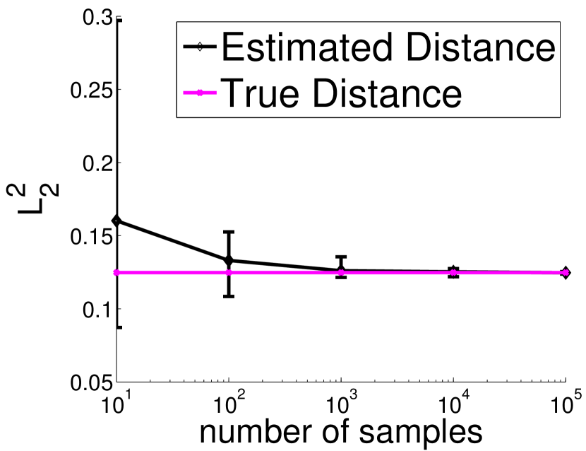
(a) Two 1D Gaussian distributions with different means.

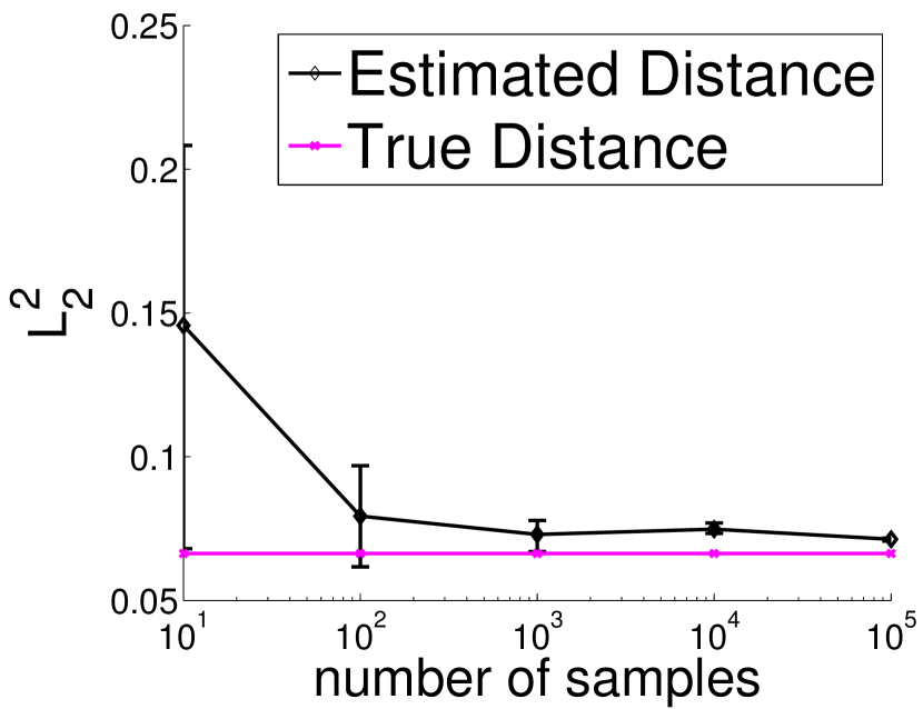
(b) Two 1D Gaussian distributions with different variance.

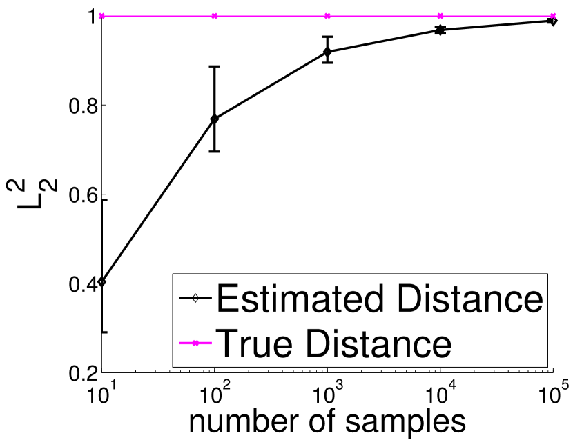
(c) Two uniform distributions with different ranges.

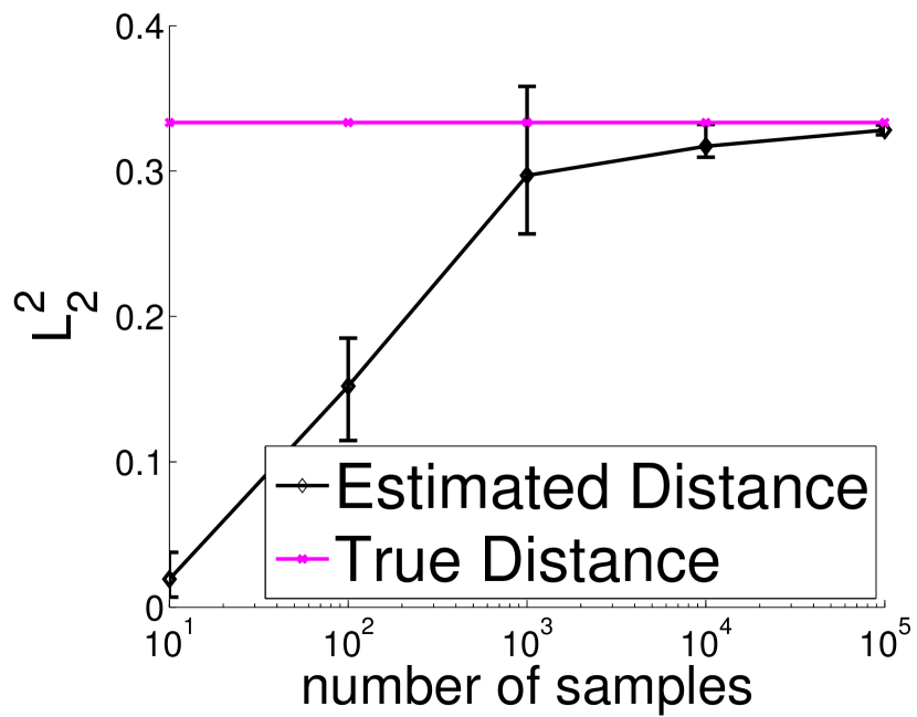
(d) One uniform distribution and one triangular distribution.

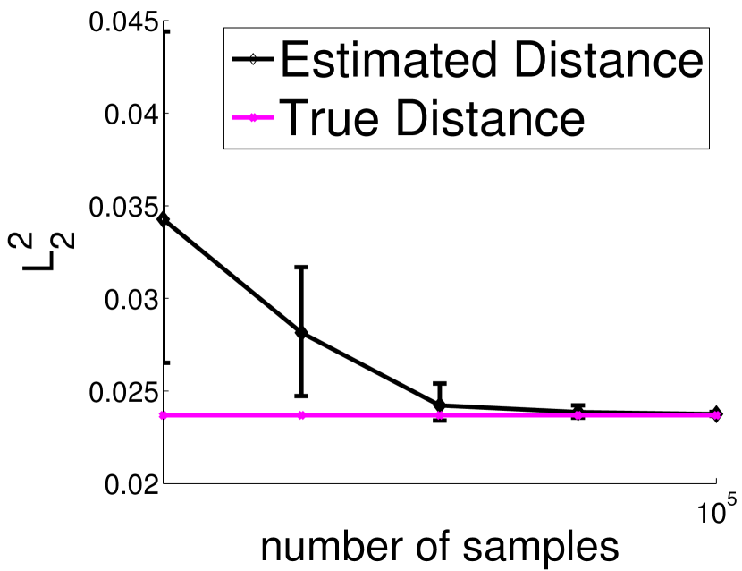
(a) Two 3D Gaussian distributions with different means.

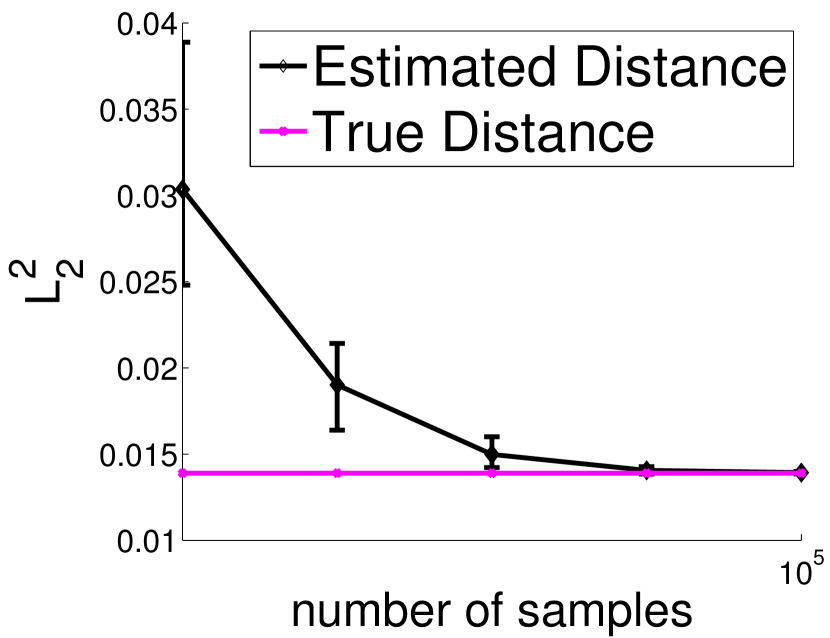
(b) Two 3D Gaussian distributions with different variance.

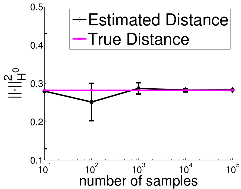
(c) Estimation of $H^{0}$ norm of $\mathcal{N}\left(0,1\right)$.

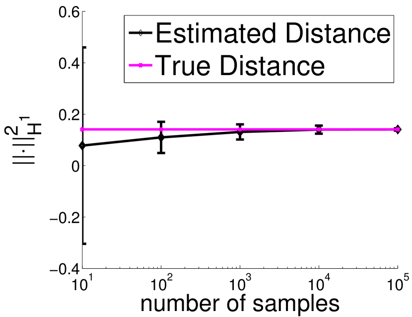
(d) Estimation of $H^{1}$ norm of $\mathcal{N}\left(0,1\right)$.

9 Connections to two-sample testing

Here, we discuss the use of our estimator in two-sample testing. There is a large literature on nonparametric two-sample testing, but we discuss only some recent approaches with theoretical connections to ours.

Let $\hat{M}$ denote our estimate of the Sobolev distance, consisting of plugging $\hat{S}$ into equation (3). Since $\|\cdot-\cdot\|_{H^{s}}$ is a metric on the space of probability density functions in $H^{s}$, computing $\hat{M}$ leads naturally to a two-sample test on this space. Theorem 5 suggests an asymptotic test, which is computationally preferable to a permutation test. In particular, for a desired Type I error rate $\alpha\in(0,1)$ our test rejects the null hypothesis $p=q$ if and only if $Q_{\chi^{2}(2Z_{n}^{D})}(T)<\alpha$.

When $s=0$, this approach is closely related to several two-sample tests in the literature based on comparing empirical characteristic functions (CFs). Originally, these tests (Heathcote, 1972; Epps and Singleton, 1986) computed the same statistic $T$ with a fixed number of random $\mathbb{R}^{D}$-valued frequencies instead of deterministic $\mathbb{Z}^{D}$-valued frequencies. This test runs in linear time, but is not generally consistent, since the two CFs need not differ almost everywhere. Recently, Chwialkowski et al. (2015) suggested using smoothed CFs, i.e., the convolution of the CF with a universal smoothing kernel $k$. This is computationally easy (due to the convolution theorem) and, when $p\neq q$, $(\widetilde{p}*k)(z)\neq(\widetilde{q}*k)(z)$ for almost all $z\in\mathbb{R}^{D}$, reducing the need for carefully choosing test frequencies. Furthermore, this test is almost-surely consistent under very general alternatives. However, it is not clear what sort of assumptions would allow finite sample analysis of the power of their test. Indeed, the convergence as $n\to\infty$ can be arbitrarily slow, depending on the random test frequencies used. Our analysis instead uses the assumption $p,q\in H^{s^{\prime}}$ to ensure that small, $\mathbb{Z}^{D}$-valued frequencies contain most of the power of $\widetilde{p}$.

These fixed-frequency approaches can be thought of as the extreme point $\theta=0$ of the computational/statistical trade-off described in section 7: they are computable in linear time and (with smoothing) are strongly consistent, but do not satisfy finite-sample bounds under general conditions.

At the other extreme ($\theta=1$) are MMD-based tests of Gretton et al. (2006, 2012), which utilize the entire spectrum $\widetilde{p}$. These tests are statistically powerful and have strong guarantees for densities in an RKHS, but have $O(n^{2})$ computational complexity. The computational/statistical trade-off discussed in Section 7 can be thought of as an interpolation (controlled by $\theta$) of these approaches, with runtime in the case $\theta=1$ approaching quadratic for large $D$ and small $s^{\prime}$.

10 Conclusions and future work

In this paper, we proposed nonparametric estimators for Sobolev inner products, norms and distances of probability densities, for which we derived finite-sample bounds and asymptotic distributions.

A natural follow-up question to our work is whether estimating smoothness of a density can guide the choice of smoothing parameters in nonparametric estimation. For some problems, such as estimating functionals of a density, this may be especially useful, since no error metric is typically available for cross-validation. Even when cross-validation is an option, as in density estimation or regression, estimating smoothness may be faster, or may suggest an appropriate range of parameter values.

Appendix A Proof of Variance Bound

Theorem 7.

(Variance Bound) If $p,q\in H^{s^{\prime}}$ for some $s^{\prime}>s$, then

$$\mathbb{V}\left[\hat{S}_{n}\right]\leq 2C_{1}\frac{Z_{n}^{4s+D}}{n^{2}}+\frac{C_{2}}{n},$$ (15)

where $C_{1}$ and $C_{2}$ are the constants (in $n$)

$$C_{1}:=\frac{2^{D}\Gamma(4s+1)}{\Gamma(4s+D+1)}\|p\|_{L^{2}}\|q\|_{L^{2}}$$

and $C_{2}:=\left(\|p\|_{H^{s}}+\|q\|_{H^{s}}\right)\|p\|_{W^{2s,4}}\|q\|_{W^{2s,4}}+\|p\|_{H^{s}}^{4}\|q\|_{H^{s}}^{4}$.

Proof: We will use the Efron-Stein inequality (Efron and Stein, 1981) to bound the variance of $\hat{S}_{n}$. To do this, suppose we were to draw $n$ additional IID samples $X_{1}^{\prime},\dots,X_{n}^{\prime}\sim p$, and define, for all $\ell,j\in\{1,\dots,n\}$,

$$X_{j}^{(\ell)}=\left\{\begin{array}[]{ll}X_{j}^{\prime}&\mbox{ if }j=\ell\\ X_{j}&\mbox{ else }\end{array}\right..$$

Let

$$\hat{S}_{n}^{(\ell)}:=\frac{1}{n^{2}}\sum_{|z|\leq Z_{n}}z^{2s}\sum_{j=1}^{n}\sum_{k=1}^{n}\psi_{z}(X_{j}^{(\ell)})\overline{\psi_{z}(Y_{k})}$$

denote our estimate when we replace $X_{\ell}$ by $X_{\ell}^{\prime}$. Noting the symmetry of $\hat{S}_{n}$ in $p$ and $q$, the Efron-Stein inequality tells us that

$$\mathbb{V}\left[\hat{S}_{n}\right]\leq\sum_{\ell=1}^{n}\mathop{\mathbb{E}}\left[\left|\hat{S}_{n}-\hat{S}_{n}^{(\ell)}\right|^{2}\right],$$ (16)

where the expectation above (and elsewhere in this section) is taken over all $3n$ samples $X_{1},\dots,X_{2n},X_{1}^{\prime},\dots,X_{2n}^{\prime},Y_{1},\dots,Y_{n}$. Expanding the difference in (16), note that any terms with $j\neq\ell$ cancel, so that

$$\hat{S}_{n}-\hat{S}_{n}^{(\ell)} =\frac{1}{n^{2}}\sum_{|z|\leq Z_{n}}z^{2s}\sum_{j=1}^{n}\sum_{k=1}^{n}\psi_{z}(X_{j})\overline{\psi_{z}(Y_{k})}-\psi_{z}(X_{j}^{(\ell)})\overline{\psi_{z}(Y_{k})}$$

$$=\frac{1}{n^{2}}\sum_{|z|\leq Z_{n}}z^{2s}(\psi_{z}(X_{\ell})-\psi_{z}(X_{\ell}^{\prime}))\sum_{k=1}^{n}\psi_{-z}(Y_{k}),$$

and so

$$\left|\hat{S}_{n}-\hat{S}_{n}^{(\ell)}\right|^{2}$$

$$=\frac{1}{n^{4}}\sum_{|y|,|z|\leq Z_{n}}(yz)^{2s}(\psi_{y}(X_{\ell})-\psi_{y}(X_{\ell}^{\prime}))(\psi_{-z}(X_{\ell})-\psi_{-z}(X_{\ell}^{\prime}))\left(\sum_{k=1}^{n}\psi_{-y}(Y_{k})\right)\left(\sum_{k=1}^{n}\psi_{z}(Y_{k})\right).$$ (17)

Since $X_{\ell}$ and $X_{\ell}^{\prime}$ are IID,

$$\mathop{\mathbb{E}}\left[(\psi_{y}(X_{\ell})-\psi_{y}(X_{\ell}^{\prime}))(\psi_{-z}(X_{\ell})-\psi_{-z}(X_{\ell}^{\prime}))\right] =2\left(\mathop{\mathbb{E}}_{X\sim p}\left[\psi_{y-z}(X)\right]-\mathop{\mathbb{E}}_{X\sim p}\left[\psi_{y}(X)\right]\mathop{\mathbb{E}}_{X\sim p}\left[\psi_{-z}(X)\right]\right)$$

$$=2\left(\widetilde{p}(y-z)-\widetilde{p}(y)\widetilde{p}(-z)\right),$$

and, since $Y_{1},\dots,Y_{n}$ are IID,

$$\mathop{\mathbb{E}}\left[\left(\sum_{k=1}^{n}\psi_{-y}(Y_{k})\right)\left(\sum_{k=1}^{n}\psi_{z}(Y_{k})\right)\right] =n\mathop{\mathbb{E}}_{Y\sim q}\left[\psi_{z-y}(Y)\right]+n(n-1)\mathop{\mathbb{E}}_{Y\sim q}\left[\psi_{-y}(Y)\right]\mathop{\mathbb{E}}_{Y\sim q}\left[\psi_{z}(Y)\right]$$

$$=n\widetilde{q}(z-y)+n(n-1)\widetilde{q}(-y)\widetilde{q}(z).$$

In view of these two equalities, taking the expectation of (17) and using the fact that $X_{\ell}$ and $X_{\ell}^{\prime}$ are independent of $X_{n+1},\dots,X_{2n}$, (17) reduces:

$$\mathop{\mathbb{E}}\left[\left|\hat{S}_{n}-\hat{S}_{n}^{(\ell)}\right|^{2}\right]=\frac{2}{n^{3}}\sum_{|y|,|z|\leq Z_{n}}(yz)^{2s}\left(\widetilde{p}(y-z)-\widetilde{p}(y)\widetilde{p}(-z)\right)\left(\widetilde{q}(z-y)+(n-1)\widetilde{q}(-y)\widetilde{q}(z)\right)$$

$$=\frac{2}{n^{3}}\sum_{|y|,|z|\leq Z_{n}}(yz)^{2s}\left(\widetilde{p}(y-z)\widetilde{q}(z-y)-\widetilde{p}(y)\widetilde{p}(-z)\widetilde{q}(z-y)\right.$$

$$\hskip 99.58464pt\left.+(n-1)\widetilde{p}(y-z)\widetilde{q}(-y)\widetilde{q}(z)-(n-1)\widetilde{p}(y)\widetilde{p}(-z)\widetilde{q}(-y)\widetilde{q}(z)\right).$$ (18)

We now need to bound following terms in magnitude:

$$\sum_{|y|,|z|\leq Z_{n}}(yz)^{2s}\widetilde{p}(y-z)\widetilde{q}(z-y),\quad$$ (19)

$$\sum_{|y|,|z|\leq Z_{n}}(yz)^{2s}\widetilde{p}(y-z)\widetilde{q}(-y)\widetilde{q}(z),$$ (20)

and $$\sum_{|y|,|z|\leq Z_{n}}(yz)^{2s}\widetilde{p}(y)\widetilde{p}(-z)\widetilde{q}(-y)\widetilde{q}(z)$$ (21)

(the second term in (18) is bounded identically to the third term).

To bound (19), we perform a change of variables, replacing $y$ by $k=y-z$:

$$\sum_{|y|,|z|\leq Z_{n}}(yz)^{2s}\widetilde{p}(y-z)\widetilde{q}(z-y) =\sum_{|k|\leq 2Z_{n}}\widetilde{p}(k)\widetilde{q}(-k)\sum_{j=1}^{D}\sum_{z_{j}=\max\{-Z_{n},k_{j}-Z_{n}\}}^{\min\{Z_{n},k_{j}+Z_{n}\}}((k-z)z)^{2s}$$ (22)

$$\leq\frac{2^{D}\Gamma(4s+1)}{\Gamma(4s+D+1)}Z_{n}^{4s+D}\sum_{|k|\leq 2Z_{n}}\widetilde{p}(k)\widetilde{q}(-k)$$ (23)

$$\leq C_{1}Z_{n}^{4s+D},$$ (24)

where $C_{1}$ is the constant (in $n$ and $Z_{n}$)

$$C_{1}:=\frac{2^{D}\Gamma(4s+1)}{\Gamma(4s+D+1)}\|p\|_{2}\|q\|_{2}.$$ (25)

(22) and (23) follow from observing that

$$\sum_{j=1}^{D}\sum_{z_{j}=\max\{-Z_{n},k_{j}-Z_{n}\}}^{\min\{Z_{n},k_{j}+Z_{n}\}}((k_{j}-z_{j})z_{j})^{2s}=(f*f)(k_{j}),$$

where $f(z):=z^{2s}1_{\{|z|\leq Z_{n}\}},\forall z\in\mathbb{Z}^{D}$ and $*$ denotes convolution (over $\mathbb{Z}^{D}$). This convolution is clearly maximized when $k=0$, in which case

$$(f*f)(k)=\sum_{|z|\leq Z_{n}}z^{4s}\leq\left(\int_{B_{\infty}(0,Z_{n})}z^{4s}\,dz\right)=\frac{2^{D}\Gamma(4s+1)}{\Gamma(4s+D+1)}Z_{n}^{4s+D},$$

where we upper bounded the series by an integral over

$$B_{\infty}(0,Z_{n}):=\{z\in\mathbb{R}^{D}:\|z\|_{\infty}=\max\{|z_{1}|,...,|z_{D}|\}\leq Z_{n}\}.$$

(24) then follows via Cauchy-Schwarz.

Bounding (20) for general $s$ is more involved and requires rigorously defining more elaborate notions from the theory distributions, but the basic idea is as follows:

$$\sum_{|y|,|z|\leq Z_{n}}(yz)^{2s}\widetilde{p}(y-z)\widetilde{q}(-y)\widetilde{q}(z) =\sum_{|y|\leq Z_{n}}y^{2s}\widetilde{q}(-y)\sum_{|z|\leq Z_{n}}z^{2s}\widetilde{p}(y-z)\widetilde{q}(z)$$

$$=\sum_{|y|,|z|\leq Z_{n}}y^{2s}\widetilde{q}(-y)\widetilde{\left(p_{n}^{(s)}q_{n}^{(s)}\right)}(y)$$

$$\leq\sqrt{\sum_{|y|\leq Z_{n}}y^{2s}\left|\widetilde{q}(y)\right|^{2}\sum_{|y|\leq Z_{n}}y^{2s}\left(\widetilde{\left(p^{(s)}q^{(s)}\right)}(y)\right)^{2}}$$

$$=\|q\|_{H^{s}}\|p_{n}^{(s)}q_{n}^{(s)}\|_{H^{s}}\leq\|q\|_{H^{s}}\|p_{n}\|_{W^{2s,4}}\|q_{n}\|_{W^{2s,4}}.$$ (26)

Here, $p_{n}^{(s)}$ and $q_{n}^{(s)}$ denote $s$-order fractional derivatives of $p_{n}$ and $q_{n}$, respectively, and $W^{2s,4}$ is a Sobolev space (with associated pseudonorm $\|\cdot\|_{W^{2s,4}}$), which can be informally thought of as $W^{2s,4}:=\left\{p\in L^{2}:\left(p^{(s)}\right)^{2}\in H^{s}\right\}$. The equality between the first and second lines follows from Theorem 10, and both inequalities are simply applications of Cauchy-Schwarz. For sake of intuition, it can be noted that the above steps are relatively elementary when $s=0$. Now, it suffices to note that, by the Rellich-Kondrachov embedding theorem (Rellich, 1930; Evans, 2010), $W^{2s,4}\subseteq H^{s^{\prime}}$, and hence $\|p_{n}\|_{W^{2s,4}}\leq\|p\|_{W^{2s,4}}<\infty$, as long as $s^{\prime}\geq 2s+\frac{D}{4}$.

Bounding (21) is a simple application of Cauchy-Schwarz:

$$\sum_{|y|,|z|\leq Z_{n}}(yz)^{2s}\widetilde{p}(y)\widetilde{p}(-z)\widetilde{q}(-y)\widetilde{q}(z) =\left(\sum_{|y|\leq Z_{n}}y^{2s}\widetilde{p}(y)\widetilde{q}(-y)\right)\left(\sum_{|z|\leq Z_{n}}z^{2s}\widetilde{p}(-z)\widetilde{q}(z)\right)$$

$$\leq\left(\sum_{|z|\leq Z_{n}}z^{2s}\left|\widetilde{p}(z)\right|^{2}\right)^{2}\left(\sum_{|z|\leq Z_{n}}z^{2s}\left|\widetilde{q}(z)\right|^{2}\right)^{2}$$

$$=\|p\|_{H^{s}}^{4}\|q\|_{H^{s}}^{4}$$ (27)

Plugging (24), (26), and (27) into (18) gives

$$\mathop{\mathbb{E}}\left[\left|\hat{S}_{n}-\hat{S}_{n}^{(\ell)}\right|^{2}\right]\leq 2C_{1}\frac{Z_{n}^{4s+D}}{n^{3}}+\frac{C_{2}}{n^{2}},$$

where $C_{2}$ denotes the constant (in $n$ and $Z_{n}$)

$$C_{2}:=\left(\|p\|_{H^{s}}+\|q\|_{H^{s}}\right)\|p\|_{W^{2s,4}}\|q\|_{W^{2s,4}}+\|p\|_{H^{s}}^{4}\|q\|_{H^{s}}^{4}.$$ (28)

Plugging this into the Efron-Stein inequality (16) gives, by symmetry of $\hat{S}_{n}$ in $X_{1},...,X_{n}$,

$$\mathbb{V}\left[\hat{S}_{n}\right]\leq 2C_{1}\frac{Z_{n}^{4s+D}}{n^{2}}+\frac{C_{2}}{n}.$$

 

Appendix B Proofs of Asymptotic Distributions

Theorem 8.

Suppose that, for some $s^{\prime}>2s+\frac{D}{4}$, $p,q\in H^{s^{\prime}}$, and suppose $Z_{n}n^{\frac{1}{4(s-s^{\prime})}}\to\infty$ and $Z_{n}n^{-\frac{1}{4s+D}}\to 0$ as $n\to\infty$. Then, $\hat{S}_{n}$ is asymptotically normal with mean $\langle p,q\rangle$. In particular, for $j\in\{1,\dots,n\}$, define the following quantities:

$$W_{j}:=\begin{bmatrix}Z_{n}^{s}e^{iZ_{n}X_{j}}\\ \vdots\\ e^{iX_{j}}\\ e^{iX_{j}}\\ \vdots\\ Z_{n}^{s}e^{-iZ_{n}X_{j}}\end{bmatrix},\quad V_{j}:=\begin{bmatrix}Z_{n}^{s}e^{iZ_{n}Y_{j}}\\ \vdots\\ e^{iY_{j}}\\ e^{iY_{j}}\\ \vdots\\ Z_{n}^{s}e^{-iZ_{n}Y_{j}}\end{bmatrix},\quad\overline{W}:=\frac{1}{n}\sum_{j=1}^{n}W_{j},\quad\overline{V}:=\frac{1}{n}\sum_{j=1}^{n}V_{j}\in\mathbb{R}^{2Z_{n}},$$

$$\Sigma_{W}:=\frac{1}{n}\sum_{j=1}^{n}(W_{j}-\overline{W})(W_{j}-\overline{W})^{T},\quad\mbox{ and }\quad\Sigma_{V}:=\frac{1}{n}\sum_{j=1}^{n}(V_{j}-\overline{V})(V_{j}-\overline{V})^{T}\in\mathbb{R}^{2Z_{n}\times 2Z_{n}}.$$

Then, for

$$\hat{\sigma}_{n}^{2}:=\begin{bmatrix}\overline{V}\\ \overline{W}\end{bmatrix}^{T}\begin{bmatrix}\Sigma_{W}&0\\ 0&\Sigma_{V}\end{bmatrix}\begin{bmatrix}\overline{V}\\ \overline{W}\end{bmatrix},$$

we have

$$\sqrt{n}\left(\frac{\hat{S}_{n}-\langle p,q\rangle_{H^{s}}}{\hat{\sigma}_{n}}\right)\stackrel{{\scriptstyle D}}{{\to}}\mathcal{N}(0,1).$$

Proof: By the bias bound and the assumption $Z_{n}^{4(s-s^{\prime})}n\to\infty$, it suffices to show

$$\sqrt{n}\left(\frac{\hat{S}_{n}-\mathop{\mathbb{E}}\left[\hat{S}_{n}\right]}{\sigma_{n}}\right)\stackrel{{\scriptstyle D}}{{\to}}\mathcal{N}(0,1).\quad\mbox{ as }\quad n\to\infty.$$ (29)

Let

$$\widetilde{p}_{Z_{n}}:=\begin{bmatrix}\widetilde{p}(-Z_{n})\\ \widetilde{p}(-Z_{n}+1)\\ \vdots\\ \widetilde{p}(Z_{n}-1)\\ \widetilde{p}(Z_{n})\\ \end{bmatrix},\quad\hat{p}_{Z_{n}}:=\begin{bmatrix}\hat{p}(-Z_{n})\\ \hat{p}(-Z_{n}+1)\\ \vdots\\ \hat{p}(Z_{n}-1)\\ \hat{p}(Z_{n})\\ \end{bmatrix},$$

$$\widetilde{q}_{Z_{n}}:=\begin{bmatrix}\widetilde{q}(-Z_{n})\\ \widetilde{q}(-Z_{n}+1)\\ \vdots\\ \widetilde{q}(Z_{n}-1)\\ \widetilde{q}(Z_{n})\\ \end{bmatrix},\quad\mbox{ and }\quad\hat{q}:=\begin{bmatrix}\hat{q}(-Z_{n})\\ \hat{q}(-Z_{n}+1)\\ \vdots\\ \hat{q}(Z_{n}-1)\\ \hat{q}(Z_{n})\\ \end{bmatrix}.$$

Since $\hat{p}_{Z_{n}}$ and $\hat{q}_{Z_{n}}$ are empirical means of bounded random vectors with means $\widetilde{p}_{Z_{n}}$ and $\widetilde{q}_{Z_{n}}$, respectively, by the central limit theorem, as $n\to\infty$,

$$\sqrt{n}\left(\hat{p}_{Z_{n}}-\widetilde{p}_{Z_{n}}\right)\stackrel{{\scriptstyle D}}{{\to}}\mathcal{N}(0,\Sigma_{p})\quad\mbox{ and }\quad\sqrt{n}\left(\hat{q}_{Z_{n}}-\widetilde{q}_{Z_{n}}\right)\stackrel{{\scriptstyle D}}{{\to}}\mathcal{N}(0,\Sigma_{q}),$$

where

$$\left(\Sigma_{p}\right)_{w,z}:=\operatornamewithlimits{Cov}_{X\sim p}\left(\psi_{w}(X),\psi_{z}(X)\right)\quad\mbox{ and }\quad\left(\Sigma_{q}\right)_{w,z}:=\operatornamewithlimits{Cov}_{X\sim q}\left(\psi_{w}(X),\psi_{z}(X)\right).$$

Define $h:\mathbb{R}^{2Z_{n}+1}\times\mathbb{R}^{2Z_{n}+1}\to\mathbb{R}$ by $h(x,y)=\sum_{z=-Z_{n}}^{Z_{n}}z^{2s}x_{z}y_{-z}$, and note that

$$\sigma_{n}^{2}:=\left(\nabla h\left(\widetilde{p}_{Z_{n}},\widetilde{q}_{Z_{n}}\right)\right)^{\prime}\begin{bmatrix}\Sigma_{p}&0\\ 0&\Sigma_{q}\end{bmatrix}\left(\nabla h\left(\widetilde{p}_{Z_{n}},\widetilde{q}_{Z_{n}}\right)\right).$$

(29) follows by the delta method.  

Theorem 9.

Suppose that, for some $s^{\prime}>2s+\frac{D}{4}$, $p,q\in H^{s^{\prime}}$, and suppose $Z_{n}n^{\frac{1}{4(s-s^{\prime})}}\to\infty$ and $Z_{n}n^{-\frac{1}{4s+D}}\to 0$ as $n\to\infty$. For $j\in\{1,\dots,n\}$, define

$$W_{j}:=\begin{bmatrix}Z_{n}^{s}\left(e^{iZ_{n}X_{j}}-e^{iZ_{n}Y_{j}}\right)\\ \vdots\\ e^{iX_{j}}-e^{iY_{j}}\\ e^{-iX_{j}}-e^{-iY_{j}}\\ \vdots\\ Z_{n}^{s}\left(e^{-iZ_{n}X_{j}}-e^{-iZ_{n}Y_{j}}\right)\end{bmatrix}\in\mathbb{R}^{2Z_{n}}.$$

Let

$$\overline{W}:=\frac{1}{n}\sum_{j=1}^{n}W_{j}\quad\mbox{ and }\quad\Sigma:=\frac{1}{n}\sum_{j=1}^{n}\left(W_{j}-\overline{W}\right)\left(W_{j}-\overline{W}\right)^{T}$$

denote the empirical mean and covariance of $W$, and define $T:=n\overline{W}^{T}\Sigma^{-1}\overline{W}$. Then, if $p=q$, then

$$Q_{\chi^{2}(2Z_{n})}(T)\stackrel{{\scriptstyle D}}{{\to}}\operatorname{Uniform}([0,1])\quad\mbox{ as }\quad n\to\infty,$$

where $Q_{\chi^{2}(2Z_{n})}:[0,\infty)\to[0,1]$ denotes the quantile function (inverse CDF) of the $\chi^{2}$ distribution $\chi^{2}(2Z_{n})$ with $2Z_{n}$ degrees of freedom.

Proof: Since, as shown in the proof of the previous theorem, the distance estimate is a sum of squared asymptotically normal, zero-mean random variables, this is a standard result in multivariate statistics. See, for example, Theorem 5.2.3 of Anderson (2003).  

Appendix C Generalizations: Weak and Fractional Derivatives

As mentioned in the main text, our estimator and analysis can be generalized nicely to non-integer $s$ using an appropriate notion of fractional derivative.

For non-negative integers $s$, let $\delta^{(s)}$ denote the measure underlying of the $s$-order derivative operator at $0$; that is, $\delta^{(s)}$ is the distribution such that

$$\int_{\mathbb{R}}f(x)\delta^{(s)}(x)\,dx=f^{(s)}(0),$$

for all test functions $f\in H^{s}$. Then, for all $z\in\mathbb{R}$, the Fourier transform of $\delta^{(s)}$ is

$$\widetilde{\delta}(z)=\int_{\mathbb{R}}e^{-izx}\delta^{(s)}(x)\,dx=(-iz)^{s}.$$

Thus, we can naturally generalize the derivative operator $\delta^{(s)}$ to general $s\in[0,\infty)$ as the inverse Fourier transform of the function $z\mapsto(-iz)^{s}$. Generalization to differentiation at an arbitrary $y\in\mathbb{R}$ follows from translation properties of the Fourier transform, and, in multiple dimensions, for $s\in\mathbb{R}^{D}$, we can consider the inverse Fourier transform of $z\in\mathbb{R}^{D}\mapsto\prod_{j=1}^{D}(iz_{j})^{s_{j}}$.

With this definition in place, we can prove the following the Convolution Theorem, which equates a particular weighted convolution of Fourier transforms and a product of particular fractional derivatives. Note that we will only need this result in the case that $f$ is a trigonometric polynomial (i.e., $\widetilde{f}$ has finite support), because we apply it only to $p_{n}$ and $q_{n}$. Hence, the sum below has only finitely many non-zero terms and commutes freely with integrals.

Theorem 10.

Suppose $p,q\in L^{2}$ are trigonometric polynomials. Then, $\forall s\in[0,\infty)$, and $y\in\mathbb{Z}^{D}$,

$$\sum_{z\in\mathbb{Z}^{D}}z^{2s}\widetilde{p}(y-z)\widetilde{q}(z)=\widetilde{\left(p^{(s)}q^{(s)}\right)}(y).$$

Proof: By linearity of the integral,

$$\sum_{z\in\mathbb{Z}^{D}}z^{2s}\widetilde{p}(y-z)\widetilde{q}(z) =\sum_{z\in\mathbb{Z}^{D}}z^{2s}\int_{\mathbb{R}^{D}}p(x_{1})e^{-i\langle y-z,x_{1}\rangle}\,dx_{1}\int_{\mathbb{R}^{D}}q(x_{2})e^{-i\langle z,x_{2}\rangle}\,dx_{2}$$

$$=\int_{\mathbb{R}^{D}}\int_{\mathbb{R}^{D}}p(x_{1})q(x_{2})e^{-i\langle y,x_{1}\rangle}\sum_{z\in\mathbb{Z}^{D}}z^{2s}e^{i\langle z,x_{1}-x_{2}\rangle}\,dx_{1}\,dx_{2}$$

$$=\int_{\mathbb{R}^{D}}\int_{\mathbb{R}^{D}}p(x_{1})q(x_{2})e^{-i\langle y,x_{1}\rangle}\delta^{(s)}(x_{1}-x_{2})\,dx_{1}\,dx_{2}$$

$$=\int_{\mathbb{R}^{D}}p^{(s)}(x)q^{(s)}(x)e^{-i\langle y,x\rangle}\,dx=\widetilde{\left(p^{(s)}q^{(s)}\right)}(y).$$

 

Acknowledgments

This material is based upon work supported by a National Science Foundation Graduate Research Fellowship to the first author under Grant No. DGE-1252522.

References

- Anderson et al. (1994) Niall H Anderson, Peter Hall, and D Michael Titterington. Two-sample test statistics for measuring discrepancies between two multivariate probability density functions using kernel-based density estimates. Journal of Multivariate Analysis, 50(1):41–54, 1994.
- Anderson (2003) TW Anderson. An introduction to multivariate statistical analysis. Wiley, 2003.
- Bickel and Ritov (1988) Peter J Bickel and Ya’acov Ritov. Estimating integrated squared density derivatives: sharp best order of convergence estimates. Sankhyā: The Indian Journal of Statistics, Series A, pages 381–393, 1988.
- Birgé and Massart (1995) Lucien Birgé and Pascal Massart. Estimation of integral functionals of a density. The Annals of Statistics, pages 11–29, 1995.
- Chwialkowski et al. (2015) Kacper P Chwialkowski, Aaditya Ramdas, Dino Sejdinovic, and Arthur Gretton. Fast two-sample testing with analytic representations of probability measures. In Advances in Neural Information Processing Systems, pages 1972–1980, 2015.
- Efron and Stein (1981) Bradley Efron and Charles Stein. The jackknife estimate of variance. The Annals of Statistics, pages 586–596, 1981.
- Epps and Singleton (1986) TW Epps and Kenneth J Singleton. An omnibus test for the two-sample problem using the empirical characteristic function. Journal of Statistical Computation and Simulation, 26(3-4):177–203, 1986.
- Evans (2010) Lawrence C Evans. Partial differential equations. American Mathematical Society, 2010.
- Giné and Nickl (2008) Evarist Giné and Richard Nickl. A simple adaptive estimator of the integrated square of a density. Bernoulli, pages 47–61, 2008.
- Goria et al. (2005) M. N. Goria, N. N. Leonenko, V. V. Mergel, and P. L. Novi Inverardi. A new class of random vector entropy estimators and its applications in testing statistical hypotheses. J. Nonparametric Statistics, 17:277–297, 2005.
- Gretton et al. (2006) Arthur Gretton, Karsten M Borgwardt, Malte Rasch, Bernhard Schölkopf, and Alex J Smola. A kernel method for the two-sample-problem. In Advances in neural information processing systems, pages 513–520, 2006.
- Gretton et al. (2012) Arthur Gretton, Karsten M Borgwardt, Malte J Rasch, Bernhard Schölkopf, and Alexander Smola. A kernel two-sample test. The Journal of Machine Learning Research, 13(1):723–773, 2012.
- Hall and Marron (1987) Peter Hall and James Stephen Marron. Estimation of integrated squared density derivatives. Statistics & Probability Letters, 6(2):109–115, 1987.
- Heathcote (1972) CE Heathcote. A test of goodness of fit for symmetric random variables. Australian Journal of Statistics, 14(2):172–181, 1972.
- Hero et al. (2002) A. O. Hero, B. Ma, O. J. J. Michel, and J. Gorman. Applications of entropic spanning graphs. IEEE Signal Processing Magazine, 19(5):85–95, 2002.
- Ibragimov and Khasminskii (1978) IA Ibragimov and RZ Khasminskii. On the nonparametric estimation of functionals. In Symposium in Asymptotic Statistics, pages 41–52, 1978.
- Kandasamy et al. (2015) Kirthevasan Kandasamy, Akshay Krishnamurthy, Barnabas Poczos, Larry Wasserman, et al. Nonparametric von mises estimators for entropies, divergences and mutual informations. In Advances in Neural Information Processing Systems, pages 397–405, 2015.
- Kreiss and Oliger (1979) Heinz-Otto Kreiss and Joseph Oliger. Stability of the Fourier method. SIAM Journal on Numerical Analysis, 16(3):421–433, 1979.
- Krishnamurthy et al. (2014a) Akshay Krishnamurthy, Kirthevasan Kandasamy, Barnabas Poczos, and Larry Wasserman. On estimating divergence. arXiv preprint arXiv:1410.8372, 2014a.
- Krishnamurthy et al. (2014b) Akshay Krishnamurthy, Kirthevasan Kandasamy, Barnabas Poczos, and Larry Wasserman. Nonparametric estimation of renyi divergence and friends. arXiv preprint arXiv:1402.2966, 2014b.
- Laurent (1992) Béatrice Laurent. Efficient estimation of integral functionals of a density. Université de Paris-sud, Département de mathématiques, 1992.
- Laurent et al. (1996) Béatrice Laurent et al. Efficient estimation of integral functionals of a density. The Annals of Statistics, 24(2):659–681, 1996.
- Leonenko et al. (2008) Nikolai Leonenko, Luc Pronzato, Vippal Savani, et al. A class of rényi information estimators for multidimensional densities. The Annals of Statistics, 36(5):2153–2182, 2008.
- Leoni (2009) Giovanni Leoni. A first course in Sobolev spaces, volume 105. American Mathematical Society Providence, RI, 2009.
- Moon and Hero (2014a) Kevin Moon and Alfred Hero. Multivariate f-divergence estimation with confidence. In Advances in Neural Information Processing Systems, pages 2420–2428, 2014a.
- Moon and Hero (2014b) Kevin R Moon and Alfred O Hero. Ensemble estimation of multivariate f-divergence. In Information Theory (ISIT), 2014 IEEE International Symposium on, pages 356–360. IEEE, 2014b.
- Moon et al. (2016) Kevin R Moon, Kumar Sricharan, Kristjan Greenewald, and Alfred O Hero III. Improving convergence of divergence functional ensemble estimators. arXiv preprint arXiv:1601.06884, 2016.
- Pardo (2005) Leandro Pardo. Statistical inference based on divergence measures. CRC Press, 2005.
- Póczos and Schneider (2011) Barnabás Póczos and Jeff G Schneider. On the estimation of alpha-divergences. In International Conference on Artificial Intelligence and Statistics, pages 609–617, 2011.
- Póczos et al. (2012a) Barnabás Póczos, Liang Xiong, and Jeff Schneider. Nonparametric divergence estimation with applications to machine learning on distributions. arXiv preprint arXiv:1202.3758, 2012a.
- Póczos et al. (2012b) Barnabás Póczos, Liang Xiong, Dougal J Sutherland, and Jeff Schneider. Nonparametric kernel estimators for image classification. In Computer Vision and Pattern Recognition (CVPR), 2012 IEEE Conference on, pages 2989–2996. IEEE, 2012b.
- Principe (2010) Jose C Principe. Information theoretic learning: Renyi’s entropy and kernel perspectives. Springer Science & Business Media, 2010.
- Quadrianto et al. (2009) Novi Quadrianto, James Petterson, and Alex J Smola. Distribution matching for transduction. In Advances in Neural Information Processing Systems, pages 1500–1508, 2009.
- Ram et al. (2009) Parikshit Ram, Dongryeol Lee, William March, and Alexander G Gray. Linear-time algorithms for pairwise statistical problems. In Advances in Neural Information Processing Systems, pages 1527–1535, 2009.
- Rellich (1930) Franz Rellich. Ein satz über mittlere konvergenz. Nachrichten von der Gesellschaft der Wissenschaften zu Göttingen, Mathematisch-Physikalische Klasse, 1930:30–35, 1930.
- Schweder (1975) Tore Schweder. Window estimation of the asymptotic variance of rank estimators of location. Scandinavian Journal of Statistics, pages 113–126, 1975.
- Singh and Póczos (2014a) Shashank Singh and Barnabás Póczos. Generalized exponential concentration inequality for renyi divergence estimation. In Proceedings of The 31st International Conference on Machine Learning, pages 333–341, 2014a.
- Singh and Póczos (2014b) Shashank Singh and Barnabás Póczos. Exponential concentration of a density functional estimator. In Advances in Neural Information Processing Systems, pages 3032–3040, 2014b.
- Tsybakov (2008) A.B. Tsybakov. Introduction to Nonparametric Estimation. Springer Publishing Company, Incorporated, 1st edition, 2008. ISBN 0387790519, 9780387790510.
- Wolsztynski et al. (2005) E. Wolsztynski, E. Thierry, and L. Pronzato. Minimum-entropy estimation in semi-parametric models. Signal Process., 85(5):937–949, 2005. ISSN 0165-1684. doi: http://dx.doi.org/10.1016/j.sigpro.2004.11.028.
- Zaremba et al. (2013) Wojciech Zaremba, Arthur Gretton, and Matthew Blaschko. B-test: A non-parametric, low variance kernel two-sample test. In Advances in neural information processing systems, pages 755–763, 2013.
- Zhao and Meng (2015) Ji Zhao and Deyu Meng. Fastmmd: Ensemble of circular discrepancy for efficient two-sample test. Neural computation, 27(6):1345–1372, 2015.
- Zygmund (2002) Antoni Zygmund. Trigonometric series, volume 1. Cambridge university press, 2002.