Abstract

We propose a novel modeling framework to study the effect of covariates of various types on the conditional distribution of the response. The methodology accommodates flexible model structure, allows for joint estimation of the quantiles at all levels, and provides a computationally efficient estimation algorithm. Extensive numerical investigation confirms good performance of the proposed method. The methodology is motivated by and applied to a lactating sow study, where the primary interest is to understand how the dynamic change of minute-by-minute temperature in the farrowing rooms within a day (functional covariate) is associated with low quantiles of feed intake of lactating sows, while accounting for other sow-specific information (vector covariate).

1 Introduction

Many modern applications routinely collect data on study participants comprising scalar responses and covariates of various types, vector, function, image, and the main question of interest is to examine how the covariates affect the response. For example, in our motivating experimental study the goal is to analyze how the minute-by-minute daily temperature and humidity of the farrowing rooms, where sows are placed after giving birth for nursing, affect their feed intake during a lactation period. The covariates consist of temperature profile, humidity, and sow age, where the response is a total amount of daily feed intake of sows. A popular approach in these cases is to use a nonparametric framework and assume that the mixed covariates solely affect the mean response; see Cardot et al., (1999); James, (2002); Ramsay and Silverman, (2005, 2002); Ferraty and Vieu, (2006, 2009); Goldsmith et al., (2011); McLean et al., (2014) and others. However for our application, while it is important to study the mean feed intake, animal scientists are often more concerned with the left tail of the feed intake distribution. This is because low feed intake of lactating sows could lead to many serious issues, including decrease in milk production and negative impact on the sows reproductive system; see, for reference, Quiniou and Noblet, (1999); Renaudeau and Noblet, (2001); St-Pierre et al., (2003) among others. In this paper we focus on regression models that study the effects of covariates on the entire distribution of response. Our contribution is the development of a modeling framework that accommodates a comprehensive study of various types (vector and functional) of covariates on a scalar response.

Quantile regression models the effect of scalar/vector covariates beyond the mean response, it provides a more comprehensive study of the covariates on the response, and has attracted great interest (Koenker and Bassett Jr,, 1978; Koenker,, 2005). For pre-specified quantile levels, quantile regression models the conditional quantiles of the response as a function of the observed covariates; this approach has been extended more recently to ensure non-crossing of quantile functions (Bondell et al.,, 2010). Quantile regression has been also extended to handle functional covariates. Cardot et al., (2005) discussed quantile regression models by employing a smoothing spline modeling based approach. Kato, (2012) considered the same problem and used a functional principal component (fPC) based approach. Both papers mainly discussed the case of having a single functional covariate and it is not clear how to extend them to the case where there are multiple functional covariates or mixed covariates (vector and functional).

More recently, Tang and Cheng, (2014), Lu et al., (2014), and Yu et al., (2016) studied quantile regression when the covariates are of mixed types and introduced the partial functional linear quantile regression modeling framework. The first two publications used fPC basis while the last one considered partial quantile regression (PQR) basis. These approaches all are suitable when the interest is studying the effect of covariate at a particular quantile level, and do not handle the study of covariate effects at simultaneous quantile levels due to the well-known crossing-issue.

Ferraty et al., (2005) and Chen and Müller, (2012) considered a different perspective and studied the effect of a functional predictor on the quantiles of the response by modeling the conditional distribution of the response directly. However their approach is limited to one functional predictor. In this paper we fill this gap and propose a unifying modeling framework and estimation technique that allows to study the effect of mixed type covariates (i.e. scalar, vector, and functional) on the conditional distribution of a scalar response in a computationally efficient manner.

Let $Q_{Y|X(\cdot)}(\tau)$ denote the $\tau$th conditional quantile of $Y$ given a functional covariate $X(\cdot)$, and let $F_{Y|X(\cdot)}(y)$ denote the conditional distribution of $Y$ given $X(\cdot)$. We model the conditional distribution using a generalized function-on-function regression framework, i.e., $F_{Y|X(\cdot)}(y)=E[\mathbbm{1}(Y\leq y)|X(\cdot)]=g^{-1}\{\int X(t)\beta(t,y)dt\}$, where $\mathbbm{1}(\cdot)$ is an indicator function, $g$ is the logit link function, and we study the conditional quantiles by exploiting the relationship between $Q_{Y|X(\cdot)}(\tau)$ and $F_{Y|X(\cdot)}(y)$ through $Q_{Y|X)(\cdot)}(\tau)=\text{inf}\{y:F_{Y|X(\cdot)}(y)\geq\tau\}$ for $0<\tau<1$. The advantage and contribution of our proposed method mainly come from the following reasons: (1) our modeling approach is spline-based, and as a result it can easily accommodate smooth effects of scalar variables as well as of functional covariates; and (2) our estimation approach is based on a single step function-on-function (or function-on-scalar) penalized regression, which enables efficient implementation by exploiting off-the-shelf software and leads to competitive computations.

The remainder of the paper is structured as follows. Section 2 discusses the details of the proposed method and Section 3 describes the estimation procedure and extensions. Section 4 performs a thorough simulation study evaluating the performance of the proposed method and its competitors. We apply the proposed method to analyze the sow data in Section 5. We conclude the paper with a discussion in Section 6.

2 Methodology

2.1 Statistical framework

Let $i$ index subjects, $j$ index repeated measurements, $n$ be the number of subjects, and $m_{i}$ be the number of observations for subject $i$. Suppose we observe $\left\{Y_{i},\mathbf{X}_{i1},X_{i2},\left\{t_{ij},X_{i3}(t_{ij})\right\}_{1\leq j\leq m_{i}}\right\}_{1\leq i\leq n}$, where $Y_{i}$ is the response, which is a scalar random variable, $\mathbf{X}_{i1}$ is a $p$-dimensional vector of nuisance covariates, $X_{i2}$ is a scalar covariate, and $X_{i3}(\cdot)$ is a functional covariate, which is assumed to be square-integrable on a closed domain $\mathcal{T}$.

We propose the following model for the conditional distribution of $Y_{i}$ given $\mathbf{X}_{i1}$, $X_{i2}$ and $X_{i3}(\cdot)$:

$$F_{Y_{i}|\mathbf{X}_{i1},X_{i2},X_{i3}(\cdot)}(y) =E\left\{\mathbbm{1}\left(Y_{i}\leq y\right)|\mathbf{X}_{i1},X_{i2},X_{i3}(\cdot)\right\}$$ (1)

$$=g^{-1}\big{\{}\beta_{0}(y)+\mathbf{X}_{i1}^{T}\boldsymbol{\beta_{1}}+X_{i2}\beta_{2}(y)+\int X_{i3}(t)\beta_{3}(t,y)dt\big{\}},$$

where $F(\cdot)$ denotes the conditional distribution function as before, $g(\cdot)$ is a known, monotone link function, namely the logit link function defined as $g(x)=\log\{x/(1-x)\}$ for arbitrary scalar $x\in[0,1]$, $\beta_{0}(\cdot)$ is an unknown and smooth functional intercept, $\boldsymbol{\beta_{1}}$ is a $p$-dimensional parameter capturing the linear additive effect of the covariate vector $\mathbf{X}_{i1}$, $\beta_{2}(\cdot)$ is an unknown and smooth function, and $\beta_{3}(\cdot,\cdot)$ is an unknown and smooth bivariate function. Here, the effect of the nuisance covariates $\mathbf{X}_{i1}$ is $\boldsymbol{\beta_{1}}$, it is assumed to be constant over $y$ while the smooth intercept $\beta_{0}(y)$ is $y$-variant. The effect of $X_{i2}$ is $\beta_{2}(y)$, which varies smoothly over $y$; $\beta_{3}(\cdot,y)$ quantifies $y$-variant linear effects of the covariate $X_{i3}(\cdot)$. If the parameter function $\beta_{2}(\cdot)$ is zero then the covariate $X_{i2}$ has no effect on the distribution of the response $Y_{i}$, which is equivalent to $X_{i2}$ having no effect on any quantile level of $Y_{i}$. Similarly, it is easy to see that a null effect, say $\beta_{3}(\cdot,\cdot)\equiv 0$, is equivalent to the case that the functional covariate $X_{i3}(\cdot)$ has no effect on any quantile level of the response. Chen and Müller, (2012) (CM, henceforth) considered a similar model, however, their approach is restrictive to a single functional covariate. We discuss the differences between their method and ours in Section 2.2

To explain our ideas, we consider the case that the functional covariates are observed without noise on a fine, regular and common grid of sampling points, i.e., $t_{ij}=t_{j}$ with $j=1,\cdots,m$ for all $i$. Bear in mind, this assumption is made for illustration only, and our framework can be extended to more general cases, including settings where the functional covariate is observed with noise and at irregular sampling points, see Section 3.3.

2.2 Modeling of the covariate effects

We model $\beta_{0}(y)$ and $\beta_{2}(y)$ by using pre-specified, truncated univariate basis. Let $\{B_{0,d_{0}}(\cdot):d_{0}=1,\ldots,\kappa_{0}\}$ and $\{B_{1,d_{1}}(\cdot):d_{1}=1,\ldots,\kappa_{1}\}$ be two bases of dimensions $\kappa_{0}$ and $\kappa_{1}$ respectively. $\beta_{0}(y)\approx\sum_{d_{0}=1}^{\kappa_{0}}B_{0,d_{0}}(y)\theta_{0,d_{0}}$ and $\beta_{2}(y)\approx\sum_{d_{1}=1}^{\kappa_{1}}B_{1,d_{1}}(y)\theta_{1,d_{1}}$, where $\theta_{0,d_{0}}$’s and $\theta_{1,d_{1}}$’s are unknown basis coefficients. We represent $\beta_{3}(t,y)$ using the tensor product of two univariate bases functions, $\{B^{t}_{2,d_{2}}(t):d_{2}=1,\ldots,\kappa_{2,t}\}$ and $\{B^{y}_{2,d^{\prime}_{2}}(y):d^{\prime}_{2}=1,\ldots,\kappa_{2,y}\}$, where $\kappa_{2,t}$ and $\kappa_{2,y}$ are the bases dimensions; $\beta_{3}(t,y)\approx\sum_{d_{2}=1}^{\kappa_{2,t}}\sum_{d^{\prime}_{2}=1}^{\kappa_{2,y}}B^{t}_{2,d_{2}}(t)B^{y}_{2,d^{\prime}_{2}}(y)\theta_{2,d_{2},d^{\prime}_{2}}$, where $\theta_{2,d_{2},d^{\prime}_{2}}$’s are unknown basis coefficients. In practice, the integration term $\int X_{i3}(t)\beta_{3}(t,y)dt$ is approximated by Riemann integration $\int X_{i3}(t)\beta_{3}(t,y)dt\approx\sum_{j=1}^{m}X_{i3}(t_{j})\beta_{3}(t_{j},y)(t_{j+1}-t_{j})$ but other numerical approximation scheme can be also used.

Define $Z_{i}(y)=\mathbbm{1}(Y_{i}\leq y)$ for $y\in\mathbbm{R}$. In practice for each $y$ in a fine grid, we view $Z_{i}(y)$ as a binary-valued random functional variable. It follows that the model (1) can be written equivalently as a generalized function-on-function regression model through relating the ‘artificial’ binary functional response $Z_{i}(y)$ and the mixed covariates $\mathbf{X}_{i1},X_{i2},X_{i3}(\cdot)$. This model can be fitted by using for example the ideas of Scheipl et al., (2016) which we briefly summarize next.

Model (1) can be represented as the following generalized additive model,

$$E[Z_{i}(y)|\mathbf{X}_{i1},X_{i2},X_{i3}(\cdot)]=g^{-1}\left\{\eta_{i}(y)\right\};$$ (2)

$$\eta_{i}(y)=\sum_{d_{0}=1}^{\kappa_{0}}B_{0,d_{0}}(y)\theta_{0,d_{0}}+\mathbf{X}_{i1}^{T}\boldsymbol{\beta_{1}}+X_{i2}\sum_{d_{1}=1}^{\kappa_{1}}B_{1,d_{1}}(y)\theta_{1,d_{1}}$$

$$\qquad\qquad\qquad+\sum_{j=1}^{m}(t_{j+1}-t_{j})X_{i3}(t_{j})\sum_{d_{2}=1}^{\kappa_{2,t}}\sum_{d^{\prime}_{2}=1}^{\kappa_{2,y}}B^{t}_{2,d_{2}}(t_{j})B^{y}_{2,d^{\prime}_{2}}(y)\theta_{2,d_{2},d^{\prime}_{2}}$$

For convenience, we use the notation $B_{X_{i2},d_{1}}(y)=X_{i2}B_{1,d_{1}}(y)$, $\widetilde{X}_{i3}(t_{j})=(t_{j+1}-t_{j})X_{i3}(t_{j})$. We let $\mathbf{B}_{0}(y)=\left\{B_{0,1}(y),\cdots,B_{0,\kappa_{0}}(y)\right\}^{T}$,
$\mathbf{B}_{i1}(y)=\left\{B_{X_{i2},1}(y),\cdots,B_{X_{i2},\kappa_{1}}(y)\right\}^{T}$, $\mathbf{B}_{2,t}(t)=\left\{B_{2,1}^{t}(t),\cdots,B_{2,\kappa_{2,t}}^{t}(t)\right\}^{T}$, $\mathbf{B}_{2,y}(y)=\left\{B_{2,1}^{y}(y),\cdots,B_{2,\kappa_{2,y}}^{y}(y)\right\}^{T}$, $\boldsymbol{\theta}_{0}=\left\{\theta_{0,1},\cdots,\theta_{0,\kappa_{0}}\right\}^{T}$, $\boldsymbol{\theta}_{1}=\left\{\theta_{1,1},\cdots,\theta_{1,\kappa_{1}}\right\}^{T}$, and $\boldsymbol{\Theta}_{2}=[\theta_{2,d_{2},d^{\prime}_{2}}]_{1\leq d_{2}\leq\kappa_{2,t},1\leq d^{\prime}_{2}\leq\kappa_{2,y}}$ is a coefficient matrix. Then $\beta_{3}(t,y)=\left\{\mathbf{B}_{2,t}(t)\otimes\mathbf{B}_{2,y}(y)\right\}^{T}\boldsymbol{\theta}_{2}$, where $\boldsymbol{\theta}_{2}$ is the vectorization of $\boldsymbol{\Theta}_{2}$. We let $\widetilde{\mathbf{X}}_{i3}(\mathbf{t})=\left\{\widetilde{X}_{i3}(t_{1}),\cdots,\widetilde{X}_{i3}(t_{m})\right\}^{T}\in\mathbbm{R}^{m}$, $\mathbf{B}_{2}(\mathbf{t},y)=\left\{\mathbf{B}_{2,t}(t_{1})\otimes\mathbf{B}_{2,y}(y),\cdots,\mathbf{B}_{2,t}(t_{m})\otimes\mathbf{B}_{2,y}(y)\right\}^{T}\in\mathbbm{R}^{m\times\kappa_{2,t}\kappa_{2,y}}$, and $\mathbf{B}_{i2}(y)=\mathbf{B}_{2}(\mathbf{t},y)^{T}\widetilde{\mathbf{X}}_{i3}(\mathbf{t})$. Now model (2) can be written as

$$E[Z_{i}(y)|\mathbf{X}_{i1},X_{i2},X_{i3}(\cdot)]=g^{-1}\left\{\mathbf{X}_{i1}^{T}\boldsymbol{\beta_{1}}+\mathbf{B}_{0}(y)^{T}\boldsymbol{\theta}_{0}+\mathbf{B}_{i1}(y)^{T}\boldsymbol{\theta}_{1}+\mathbf{B}_{i2}(y)^{T}\boldsymbol{\theta}_{2}\right\}.$$ (3)

The general idea is to set the bases dimensions $\kappa_{0}$, $\kappa_{1}$, $\kappa_{2,t}$ and $\kappa_{2,y}$ to be sufficiently large to capture the complexity of the coefficient functions and control the smoothness of the estimator through some roughness penalties. This approach of using roughness penalties has been widely used; see, for example, Eilers and Marx, (1996); Ruppert, (2002); Wood, (2003, 2006) among many others.

It is important to emphasize that even in the case of a single functional covariate, our methodology differs from (Chen and Müller,, 2012) in two directions: 1) our proposed method is based on modeling the unknown smooth coefficient functions using pre-specified basis function expansion and using penalties to control their roughness. In contrast, CM uses data-driven basis, chooses the number of basis functions through the percentage of explained variance (PVE) of the functional predictors. This key difference allows our method to accommodate covariates of different types as well as non-linear effects. 2) Our estimation approach is based on a single step penalized function-on-function regression while CM uses pointwise estimation based on functional principal component bases and thus requires fitting multiple generalized regressions. This nice feature leads to an computational advantage.

3 Estimation

3.1 Estimation via penalized log-likelihood

Let $\{y_{\ell}:\ell=1,\ldots,L\}$ be a set of equally spaced points in the range of the response variable, $Y_{i}$’s. Conditioning on $\left\{\mathbf{X}_{i1},X_{i2},X_{i3}(\cdot)\right\}$, we model $Z_{i}(y_{\ell})$ as independently distributed Bernoulli variables with mean $\mu_{i}(y_{\ell})$, where $g\{\mu_{i}(y_{\ell})\}=\eta_{i}(y_{\ell})$. The coefficients $\boldsymbol{\beta}_{1}$, $\boldsymbol{\theta}_{0}$, $\boldsymbol{\theta}_{1}$ and $\boldsymbol{\theta}_{2}$, are estimated by minimizing the penalized log-likelihood criterion,

$$-2\mathcal{L}\left(\boldsymbol{\beta}_{1},\boldsymbol{\theta}_{0},\boldsymbol{\theta}_{1},\boldsymbol{\theta}_{2}|\{Z_{i}(y_{\ell}\right):\forall i,\ell\})+\lambda_{0}P_{0}(\boldsymbol{\theta}_{0})+\lambda_{1}P_{1}(\boldsymbol{\theta}_{1})+\lambda_{2,t}P_{2,t}(\boldsymbol{\theta}_{2})+\lambda_{2,y}P_{2,y}(\boldsymbol{\theta}_{2}),$$ (4)

where $\mathcal{L}$ is the log-likelihood function of data $\{Z_{i}(y_{\ell}):\ell=1,\cdots,L\}_{1\leq i\leq n}$, $\lambda_{0}$, $\lambda_{1}$, $\lambda_{2,t}$and $\lambda_{2,y}$ are smoothing parameters, which control the balance between the model fit and its complexity, $P_{0}(\cdot)$, $P_{1}(\cdot)$, $P_{2,t}(\cdot)$ and $P_{2,y}(\cdot)$ are all penalties.

There are several choices to define the penalty matrix in nonparametric regression, see Eilers and Marx, (1996); Wood, (2006). We use quadratic penalties which penalize the size of the curvature of the estimated coefficient functions. Let $P_{0}(\boldsymbol{\theta_{0}})=\int\{\partial^{2}\beta_{0}(y)/\partial y^{2}\}^{2}dy=\boldsymbol{\theta}^{T}_{0}\mathbf{D}_{0}\boldsymbol{\theta}_{0}$, where $\mathbf{D}_{0}$ is of dimension $\kappa_{0}\times\kappa_{0}$ with its $(s,s^{\prime})$ element equal to $\int\{\partial^{2}B_{0,s}(y)/\partial y^{2}\}\{\partial^{2}B_{0,s^{\prime}}(y)/\partial y^{2}\}dy$. Similarly, $P_{1}(\boldsymbol{\theta}_{1})=\int\{\partial^{2}\beta_{2}(y)/\partial y^{2}\}^{2}dy=\boldsymbol{\theta}^{T}_{1}\mathbf{D}_{1}\boldsymbol{\theta}_{1}$, where $\mathbf{D}_{1}$ is of dimension $\kappa_{1}\times\kappa_{1}$ with its $(s,s^{\prime})$ element equal to $\int\{\partial^{2}B_{1,s}(y)/\partial y^{2}\}\{\partial^{2}B_{1,s^{\prime}}(y)/\partial y^{2}\}dy$. As $\beta_{3}(\cdot,\cdot)$ is a bivariate function, the choice of penalty implies penalizing the size of curvature in each direction respectively: $P_{2,t}(\boldsymbol{\theta_{2}})=\int\int\{\partial^{2}\beta_{3}(y,t)/\partial t^{2}\}^{2}dydt=\boldsymbol{\theta}^{T}_{2}\mathbf{D}_{2,t}\boldsymbol{\theta}_{2}$, where $\mathbf{D}_{2,t}=\mathbf{P}_{2,t}\otimes\mathbf{I}_{\kappa_{2,y}}$ is of dimension $\kappa_{2,y}\kappa_{2,t}\times\kappa_{2,y}\kappa_{2,t}$ with the $(s,s^{\prime})$ element of $\mathbf{P}_{2,t}$ equal to $\int\{\partial^{2}B^{t}_{2,s}(t)/\partial t^{2}\}\allowbreak\{\partial^{2}B^{t}_{2,s^{\prime}}(t)/\partial t^{2}\}dt$ for some orthonormal spline bases. Similarly, $P_{2,y}(\boldsymbol{\theta_{2}})=\int\int\{\partial^{2}\beta_{3}(y,t)/\partial y^{2}\}^{2}dydt=\boldsymbol{\theta}^{T}_{2}\mathbf{D}_{2,y}\boldsymbol{\theta}_{2}$, where $\mathbf{D}_{2,y}=\mathbf{I}_{\kappa_{2,t}}\otimes\mathbf{P}_{2,y}$ is of dimension $\kappa_{2,y}\kappa_{2,t}\times\kappa_{2,y}\kappa_{2,t}$ with the $(s,s^{\prime})$ element of $\mathbf{P}_{2,y}$ equal to $\int\{\partial^{2}B^{y}_{2,s}(y)/\partial y^{2}\}\{\partial^{2}\allowbreak B^{y}_{2,s^{\prime}}(y)/\partial y^{2}\}dy$.

The criterion (4) can be viewed as a penalized quasi-likelihood (PQL) of the corresponding generalized linear mixed model

$$Z_{i}(y_{\ell})|\boldsymbol{\beta}_{1},\boldsymbol{\theta}_{0},\boldsymbol{\theta}_{1},\boldsymbol{\theta}_{2} \sim \text{Bernoulli}(\mu_{i}(y_{\ell})),\quad\ell=1,\ldots,L;$$ (5)

$$\quad\boldsymbol{\theta}_{0} \sim N\Big{(}\textbf{0},\lambda_{0}^{-1}\mathbf{D}^{-}_{0}\Big{)};\quad\boldsymbol{\theta}_{1}\sim N\Big{(}\textbf{0},\lambda_{1}^{-1}\mathbf{D}^{-}_{1}\Big{)};$$

$$\quad\boldsymbol{\theta}_{2} \sim N\Big{(}\textbf{0},\mathbf{D}^{-}_{2}\Big{)},$$

where $\mathbf{D}^{-}_{0}$ is the generalized inverse matrix of $\mathbf{D}_{0}$; $\mathbf{D}^{-}_{1}$ and $\mathbf{D}^{-}_{2}=(\lambda_{2,t}\mathbf{D}_{2,t}+\lambda_{2,y}\mathbf{D}_{2,y})^{-}$ are defined similarly. Wood, (2006) discusses an alternative way to deal with the rank-deficient matrices in the context of restricted maximum likelihood (REML) estimation. Here we do not account for the dependence over $y$, see Scheipl et al., (2016) for a general formulation. See also Ivanescu et al., (2015) who uses the mixed model representation of a similar regression model to (5), but with a Gaussian functional response. The smoothing parameters are estimated using REML.

3.2 Extension to nonlinear model

One advantage of the proposed framework is that it can be easily extended to allow for more flexible effects, i.e., extending the ideas to accommodate multiple covariates, scalar or functional, and varied types of effects. In particular, the smooth effect $X_{i2}\beta_{2}(y)$ can be replaced by $h_{1}(X_{i2},y)$, and $\int X_{i3}(t)\beta_{3}(t,y)dt$ by $\int h_{2}\{X_{i3}(t),t,y\}dt$, where $h_{1}(\cdot,\cdot)$ and $h_{2}(\cdot,\cdot,\cdot)$ are unknown bivariate and trivariate smooth functions, respectively; see Scheipl et al., (2016) and Kim et al., (2018). These changes require little additional computational effort. The modeling and estimation follow roughly similar ideas as Scheipl et al., (2016). We consider the nonlinear model in the simulation study for the case of having a scalar covariate only, i.e. $h_{1}(X_{i},y)$, and the corresponding results are presented in Section LABEL:sec:_sim-sca of the Supplementary materials. The results show excellent prediction performance compared to the competitive nonlinear quantile regression method, namely Constrained B-Spline Smoothing (COBS) (Ng and Maechler,, 2007).

3.3 Extension to sparse and noisy functional covariates

In practice the functional covariates are often observed at irregular times across the units and the measurements are possibly corrupted by noises. In such case, one needs to first smooth and de-noise the trajectories before fitting. When the sampling design of the functional covariate is dense, the common approach is to smooth each trajectory using splines or local polynomial smoothing, as proposed in Ramsay and Silverman, (2005) and Zhang and Chen, (2007). When the design is sparse, the smoothing can be done by pooling all the subjects and following the PACE method proposed in Yao et al., (2005). As recovering the trajectories has been extensively discussed in the literatures, we do not review the procedures here. Instead, we discuss some available computing resources that can be used to fit these methods. In our numerical study, we used fpca.sc function in the refund R package (Huang et al.,, 2015) for recovering the latent trajectories, irrespective of a sampling design (dense or sparse). Alternatively, one can use fpca.face (Xiao et al.,, 2016) in refund for regular dense design and face.sparse (Xiao et al., 2018a, ) in the R package face (Xiao et al., 2018b, ) for irregular sparse design. Once the latent trajectories are estimated, they can be used in the fitting criterion (4).

3.4 Estimation of conditional quantile

Let $\widehat{\boldsymbol{\beta}}_{1}$, $\widehat{\boldsymbol{\theta}}_{0}$, $\widehat{\boldsymbol{\theta}}_{1}$, and $\widehat{\boldsymbol{\theta}}_{2}$ be parameter estimates in (5). It follows that the estimated distribution function $\widehat{F}_{Y_{i}|\mathbf{X}_{i1},X_{i2},X_{i3}(\cdot)}(y)$ can be obtained by plugging in the estimated coefficients. The $\tau$th conditional quantile is estimated by inverting the estimated distribution, i.e., $\widehat{Q}_{Y_{i}|\mathbf{X}_{i1},X_{i2},X_{i3}(\cdot)}(\tau)=\text{inf}\{y:\widehat{F}_{Y_{i}|\mathbf{X}_{i1},X_{i2},X_{i3}(\cdot)}(y)\geq\tau\}$. The estimated distribution function is not a monotonic function yet. In practice we suggest to first apply a monotonization method as described in the Section 3.5, and then estimate the conditional quantiles by inverting the resulting estimated distribution.

3.5 Monotonization and implementation

While a conditional quantile function is nondecreasing, the resulting estimated quantiles may not be. Two approaches are widely used: one is to monotonize the estimated conditional distribution function, and the other is to monotonize the estimated conditional quantile function. We choose the former as $\widehat{F}_{Y_{i}|\mathbf{X}_{i1},X_{i2},X_{i3}(\cdot)}(y)$ is readily available at dense grid points $y_{\ell}$’s. We use an isotonic regression model (Barlow,, 1972) for monotonization, which imposes an order restriction; this is done by using the R function isoreg. Other monotonization approaches include Chernozhukov et al., (2009), which was employed in Kato, (2012).

Our approach is implemented by first creating an artificial binary response and then fitting a penalized function-on-function regression model and using the logit link function. Fitting models in (4) can be done by extending the ideas of Ivanescu et al., (2015) for Gaussian functional response; the extension of the model to the non-Gaussian functional response has recently been studied and implemented by Scheipl et al., (2016) as the pffr function in refund package (Huang et al.,, 2015).

4 Simulation study

4.1 Simulation setting

In this section we evaluate the empirical performance of the proposed method. We present results for the case when we have both functional and scalar covariates; additional results when there is only a single scalar or a single functional covariate are discussed in the Supplementary materials, Section LABEL:sec:_sim-add.

Suppose the observed data for the $i$th subject are $[Y_{i},X_{1i},\{(W_{i1},t_{i1}),\cdots,\allowbreak(W_{im_{i}},t_{im_{i}})\}]$, $t_{ij}\in[0,10]$, where $X_{1i}\overset{i.i.d}{\sim}Unif(-16,16)$, $W_{ij}=X_{2i}(t_{ij})+\epsilon_{ij}$ for $1\leq i\leq n,1\leq j\leq m_{i}$. Let $X_{2i}(t_{ij})=\mu(t_{ij})+\sum_{k=1}^{4}\xi_{ik}\phi_{k}(t_{ij})+\epsilon_{ij}$, where $\mu(t)=t+\sin(t)$, $\phi_{k}(t)=\cos\{(k+1)\pi t/10\}/\sqrt{5}$ for odd values of $k$, $\phi_{k}(t)=\sin\{k\pi t/10\}/\sqrt{5}$ for even values of $k$, $\xi_{ik}\stackrel{{\scriptstyle iid}}{{\sim}}N(0,\lambda_{k})$, $(\lambda_{1},\lambda_{2},\lambda_{3},\lambda_{4})=\{16,9,7.56,5.06\}$, and $\epsilon_{ij}\stackrel{{\scriptstyle iid}}{{\sim}}N(0,\sigma^{2}_{\epsilon})$. We assume three cases for generating response $Y_{i}$:

1. Gaussian: $Y_{i}|X_{1i},X_{2i}(\cdot)\sim N(2\int X_{2i}(t)\beta(t)dt+2X_{1i},5^{2})$; this corresponds to the quantile regression model $Q_{Y|X_{1},X_{2}(\cdot)}(\tau)=2\int X_{2i}(t)\beta(t)dt+2X_{1i}+5\Phi^{-1}(\tau)$, where $\Phi(\cdot)$ is the distribution function of the standard normal;

2. Mixture of Gaussians:
   $Y_{i}|X_{1i},X_{2i}(\cdot)\sim 0.5N(\int X_{2i}(t)\beta(t)dt+X_{1i},1^{2})+$ $0.5$ $N(3\int X_{2i}(t)\beta(t)dt$ $+3X_{1i},4^{2})$, where the true quantiles can be approximated numerically by using qnorMix function in the R package norMix;

3. Gaussian with heterogeneous error: $Y_{i}|X_{1i},X_{2i}(\cdot)\sim N(2\int X_{2i}(t)\beta(t)dt+2X_{1i},5^{2}\int X_{2i}(t)^{2}dt/\sum_{k=1}^{4}\lambda_{k})$; the true quantiles are given by $Q_{Y|X_{1},X_{2}(\cdot)}(\tau)=2\int X_{2i}(t)\beta(t)dt+2X_{1i}+5\sqrt{\int X_{2i}(t)^{2}dt/\sum_{k=1}^{4}\lambda_{k}}\Phi^{-1}(\tau)$.

Let $\beta(t)=\sum_{k=1}^{4}\beta_{k}\phi_{k}(t)$, where $\beta_{k}=1$ for $k=1,\cdots,4$.

For each case, we use different combinations of signal to noise ratio (SNR), sample size and sampling designs to generate $500$ simulated datasets. We define SNR as $\sqrt{\sum_{k=1}^{4}\lambda_{k}}/\sigma_{\epsilon}$, and consider five levels of noise: $\textnormal{SNR}=\{150,10,5,2,1\}$. Two levels of sample size are $n=100$ and $n=1000$. Two sampling designs are considered: (i) sparse design, where $\{t_{ij}:j=1,\ldots,m\}$ are $m=15$ randomly selected points from a set of $30$ equi-spaced grids in $[0,10]$; and (ii) dense design, where the sampling points $\{t_{ij}=t_{j}:j=1,\ldots,m\}$ are $m=30$ equi-spaced time points in $[0,10]$.

The performance is evaluated on a test set of $100$ subjects, for which we have $\{X_{1i^{*}},(W_{i^{*}j},t_{i^{*}j}),j=1,\ldots,m\}$ available, in terms of mean absolute error (MAE) for quantile levels $\tau=0.05,0.1,0.25,$ and $0.5$,

$$\textnormal{MAE}(\tau)=\frac{1}{100}\sum_{i^{*}=1}^{100}|\widehat{Q}_{i^{*}}(\tau)-Q_{i^{*}}(\tau)|.$$

4.2 Competing methods

We denote the proposed method by Joint QR to emphasize the single step estimation approach. We compare our method with two alternative approaches: (1) a variant of our proposed approach using pointwise estimation, denoted by Pointwise QR. This approach consists of fitting multiple regression models with binomial link function as implemented by the penalized functional regression pfr, developed by Goldsmith et al., (2011), of the refund package for generalized scalar responses. (2) A modified version of the CM method, denoted by Mod CM, that we developed to account for additional scalar covariates, and which fits multiple generalized linear models with scalar covariates and fPC scores as predictors. (3) A linear quantile regression approach using the quantile loss function and the partial quantile regression bases for functional covariates, proposed by Yu et al., (2016) and denoted by PQR. Notice that although the formulation of the first two methods implicitly account for a varying effect of the covariates on the response distribution, they do not ensure that this effect is smooth. The third approach can only estimate a specific quantile rather than the entire conditional distribution. Note that all the competing methods are monotonized for a fair comparison.

The R function pfr can incorporate both scalar/vector and functional predictors by adopting a mixed effects model framework. The functional covariates are pre-smoothed by fPC analysis (Yao et al.,, 2005); Throughout the simulation study we fix PVE as $0.95$ for fPC analysis to determine the mumber of principal components and use REML to select the smoothing parameters for our proposed methods. Other basis settings are set to their default values. We use 100 equally-distanced points between the minimum and maximum of the observed $Y_{i}$’s to set the grid $\left\{y_{\ell}:\ell=1,\cdots,L\right\}$ for the conditional distribution function.

4.3 Simulation results

Tables 1 and 2 show the accuracy of the quantile estimation for the two cases (normal and mixture) when the functional covariate is observed sparsely and the sample size is $n=100$ (Table 1) and $n=1000$ (Table 2). Table 3 presents the estimation accuracy for the case of heteroskedasticity with sparsely observed functional covariates. The results based on dense sampling design show similar patterns and thus are relegated to the supplement, see Section LABEL:sec:_sim-den. The comparison of running times is presented in Table 4.

For the case when the response is Gaussian, Tables 1 and 2 suggest that the Joint QR typically outperforms its competitors especially for lower quantile levels ($\tau=0.05$ and $\tau=0.1$). For very small noise level (SNR$=150$), PQR performs the best, followed closely by the proposed Joint QR. The variant Pointwise QR, which has a poorer performance, is generally better than the modified CM approach. As expected, as the sample size increases ($n=1000$), all the accuracy results improve; the proposed Joint QR continues to yield most accurate quantiles for the low quantile levels. For mixture of Gaussians, the results are somewhat similar. The accuracy of the quantile estimators with the Pointwise QR improves greatly; in fact the Joint QR and Pointwise QR outperform the other approaches for quantile levels $\tau=0.05,0.1,0.25$ irrespective of the SNR. Finally, Table 3 shows that the results for Gaussian with heterogeneous error are close to those for the case of Gaussian. Again, the proposed method has competitive performance in terms of estimation accuracy.

Table 4 compares the three methods that involve estimating the conditional distribution in terms of the running time required for fitting. The times are reported based on a computer with a $2.3$ GHz CPU and $8$ GB of RAM. Not surprisingly by fitting the model a single time, Joint QR is the fastest, in some cases being order of magnitude faster than the rest. Pointwise QR can be up to twice as fast as Mod CM.

For completeness, we also compare our proposed method to the appropriate competitive methods for the cases $(1)$ when there is a single scalar covariate and $(2)$ when there is a single functional covariate. The Supplementary materials, Section LABEL:sec:_sim-sca discusses the former case and compares Joint QR and Pointwise QR with the linear quantile regression (LQR) (Koenker and Bassett Jr,, 1978), implemented by rq function in the R package quantreg, and the constrained B-splines nonparametric regression quantiles (COBS), implemented by the cobs function in the R package COBS (Ng and Maechler,, 2007), in an extensive simulation experiment that involves both linear quantile settings and nonlinear quantile settings. Overall the results show that the proposed methods have similar behavior as LQR, see Table LABEL:tab:sim2MAE. Furthermore we consider the proposed method and its variant with nonlinear modeling of the conditional distribution as discussed in Section 3.2, which we denote with Joint QR (NL) for joint fitting and Pointwise QR (NL) for pointwise fitting. Nonlinear versions of the proposed methods have an excellent MAE performance, which is comparable to or better than that of the COBS method.

Finally, Section LABEL:sec:_sim-fun in the Supplementary materials discusses the simulation study for the case of having a single functional covariate and compares the proposed methods with CM in terms of MAE as well as computation time; see results displayed in Tables LABEL:tab:_sim3MAE and LABEL:tab:sim3time. The results show that the proposed Joint QR is comparable to CM in terms of the prediction accuracy and has less computation time. In our simulation study we also consider the joint fitting of the model by treating the binary response as normal and use pffr (Ivanescu et al.,, 2015) with Gaussian link, denoted by Joint QR (G).

Table 1: Average MAE (standard error in parentheses) of the predicted $\tau$-level quantile for the case of having a scalar covariate and a sparsely observed functional covariate. Sample size $n=100$.

Distribution	SNR	Method	$\tau=0.05$	$\tau=0.1$	$\tau=0.25$	$\tau=0.5$
Normal	150	Joint QR	3.67 (0.03)	3.53 (0.03)	3.30 (0.02)	3.17 (0.02)
		Pointwise QR	4.96 (0.03)	4.61 (0.03)	4.22 (0.02)	4.18 (0.02)
		Mod CM	6.04 (0.03)	5.81 (0.03)	5.55 (0.03)	5.14 (0.03)
		PQR	3.17 (0.04)	2.71 (0.03)	2.31 (0.02)	2.16 (0.02)
Normal	10	Joint QR	6.32 (0.03)	6.00 (0.03)	5.76 (0.02)	5.73 (0.02)
		Pointwise QR	7.44 (0.04)	6.85 (0.03)	6.39 (0.03)	6.28 (0.03)
		Mod CM	8.20 (0.04)	8.10 (0.04)	8.04 (0.04)	8.01 (0.04)
		PQR	6.82 (0.05)	6.11 (0.04)	5.34 (0.03)	5.09 (0.02)
Normal	5	Joint QR	7.84 (0.04)	7.34 (0.03)	6.93 (0.03)	6.84 (0.03)
		Pointwise QR	8.91 (0.04)	8.12 (0.04)	7.45 (0.03)	7.26 (0.03)
		Mod CM	9.34 (0.04)	9.23 (0.04)	9.14 (0.05)	9.06 (0.05)
		PQR	8.68 (0.06)	7.81 (0.05)	6.74 (0.03)	6.34 (0.02)
Normal	2	Joint QR	10.05 (0.05)	9.22 (0.04)	8.47 (0.03)	8.28 (0.03)
		Pointwise QR	10.91 (0.06)	9.86 (0.04)	8.87 (0.04)	8.54 (0.03)
		Mod CM	10.85 (0.05)	10.55 (0.05)	10.34 (0.06)	10.21 (0.06)
		PQR	11.21 (0.08)	10.03 (0.06)	8.56 (0.04)	7.96 (0.03)
Normal	1	Joint QR	11.50 (0.06)	10.41 (0.05)	9.40 (0.04)	9.11 (0.03)
		Pointwise QR	12.12 (0.06)	10.88 (0.05)	9.70 (0.04)	9.30 (0.03)
		Mod CM	11.95 (0.06)	11.46 (0.06)	11.07 (0.06)	11.05 (0.07 )
		PQR	12.82 (0.08)	11.38 (0.06)	9.60 (0.04)	8.86 (0.03)
Mixture	150	Joint QR	6.92 (0.06)	6.23 (0.06)	6.16 (0.06)	4.81 (0.06)
		Pointwise QR	8.10 (0.08)	6.80 (0.06)	6.66 (0.06)	5.25 (0.06)
		Mod CM	9.18 (0.07)	8.99 (0.07)	8.93 (0.07)	7.90 (0.07)
		PQR	8.43 (0.06)	7.18 (0.04)	6.22 (0.04)	5.48 (0.14)
Mixture	10	Joint QR	9.02 (0.06)	7.95 (0.05)	7.85 (0.05)	6.19 (0.06)
		Pointwise QR	10.11 (0.07)	8.52 (0.05)	7.95 (0.05)	6.42 (0.06)
		Mod CM	11.33 (0.07)	10.95 (0.07)	10.79 (0.07)	9.80 (0.08)
		PQR	10.72 (0.08)	8.99 (0.05)	7.63 (0.04)	5.33 (0.09)
Mixture	5	Joint QR	10.18 (0.06)	8.91 (0.05)	8.53 (0.05)	6.82 (0.05)
		Pointwise QR	11.18 (0.07)	9.38 (0.05)	8.58 (0.05)	6.98 (0.05)
		Mod CM	12.19 (0.07)	11.75 (0.07)	11.52 (0.07)	10.47 (0.08)
		PQR	12.12 (0.09)	10.12 (0.06)	8.40 (0.04)	5.73 (0.07)
Mixture	2	Joint QR	11.93 (0.07)	10.26 (0.05)	9.46 (0.05)	7.61 (0.05)
		Pointwise QR	12.68 (0.08)	10.63 (0.06)	9.51 (0.05)	7.70 (0.05)
		Mod CM	13.33 (0.08)	12.60 (0.08)	12.27 (0.08)	11.08 (0.10)
		PQR	14.16 (0.10)	11.72 (0.06)	9.55 (0.04)	6.41 (0.05)
Mixture	1	Joint QR	13.17 (0.08)	11.19 (0.05)	10.06 (0.05)	8.04 (0.05)
		Pointwise QR	13.71 (0.09)	11.44 (0.06)	10.10 (0.05)	8.13 (0.05)
		Mod CM	14.16 (0.08)	13.22 (0.08)	12.71 (0.09)	11.44 (0.11)
		PQR	15.44 (0.11)	12.84 (0.07)	10.23 (0.04)	6.89 (0.04)

Table 2: Average MAE (standard error in parentheses) of the predicted $\tau$-level quantile for the case of having a scalar covariate and a sparsely observed functional covariate. Sample size $n=1000$.

Distribution	SNR	Method	$\tau=0.05$	$\tau=0.1$	$\tau=0.25$	$\tau=0.5$
Normal	150	Joint QR	1.68 (0.01)	1.65 (0.01)	1.62 (0.01)	1.60 (0.01)
		Pointwise QR	1.94 (0.01)	1.92 (0.01)	1.88 (0.01)	1.81 (0.01)
		Mod CM	1.93 (0.01)	1.88 (0.01)	1.87 (0.01)	1.87 (0.01)
		PQR	1.72 (0.01)	1.61 (0.01)	1.51 (0.01)	1.48 (0.01)
Normal	10	Joint QR	5.45 (0.02)	4.97 (0.02)	4.66 (0.02)	4.65 (0.02)
		Pointwise QR	5.64 (0.02)	5.13 (0.02)	4.78 (0.02)	4.75 (0.02)
		Mod CM	5.69 (0.02)	5.21 (0.02)	4.87 (0.02)	4.85 (0.02)
		PQR	5.85 (0.02)	5.37 (0.02)	4.81 (0.02)	4.60 (0.02)
Normal	5	Joint QR	7.34 (0.03)	6.54 (0.02)	5.94 (0.02)	5.85 (0.02)
		Pointwise QR	7.53 (0.03)	6.69 (0.02)	6.04 (0.02)	5.94 (0.02)
		Mod CM	7.53 (0.03)	6.77 (0.02)	6.18 (0.02)	6.06 (0.02)
		PQR	7.84 (0.03)	7.05 (0.02)	6.16 (0.02)	5.81 (0.02)
Normal	2	Joint QR	9.97 (0.03)	8.70 (0.03)	7.62 (0.02)	7.38 (0.02)
		Pointwise QR	10.15 (0.03)	8.85 (0.03)	7.71 (0.02)	7.45 (0.02)
		Mod CM	10.12 (0.03)	8.93 (0.03)	7.87 (0.03)	7.60 (0.03)
		PQR	10.55 (0.04)	9.34 (0.03)	7.91 (0.03)	7.34 (0.02)
Normal	1	Joint QR	11.69 (0.04)	10.10 (0.03)	8.68 (0.03)	8.32 (0.03)
		Pointwise QR	11.88 (0.04)	10.25 (0.04)	8.77 (0.03)	8.39 (0.03)
		Mod CM	11.85 (0.04)	10.37 (0.04)	8.96 (0.03)	8.57 (0.03)
		PQR	12.29 (0.04)	10.77 (0.04)	9.02 (0.03)	8.29 (0.03)
Mixture	150	Joint QR	4.56 (0.02)	4.44 (0.02)	4.33 (0.03)	3.68 (0.03)
		Pointwise QR	4.34 (0.03)	4.24 (0.02)	4.20 (0.03)	3.66 (0.04)
		Mod CM	4.68 (0.03)	4.59 (0.02)	4.38 (0.03)	4.01 (0.03)
		PQR	7.84 (0.03)	6.45 (0.02)	5.29 (0.02)	3.19 (0.01)
Mixture	10	Joint QR	7.56 (0.03)	6.79 (0.02)	6.14 (0.03)	5.02 (0.03)
		Pointwise QR	7.49 (0.03)	6.61 (0.02)	5.88 (0.03)	5.02 (0.03)
		Mod CM	7.67 (0.04)	6.97 (0.03)	6.17 (0.03)	5.52 (0.04)
		PQR	10.11 (0.04)	8.29 (0.03)	6.71 (0.02)	3.62 (0.02)
Mixture	5	Joint QR	9.20 (0.04)	7.13 (0.03)	6.94 (0.03)	5.6 (0.03)
		Pointwise QR	9.17 (0.04)	7.01 (0.03)	6.71 (0.03)	5.58 (0.03)
		Mod CM	9.32 (0.04)	7.37 (0.03)	7.08 (0.03)	6.18 (0.04)
		PQR	11.46 (0.04)	9.36 (0.03)	7.49 (0.03)	4.32 (0.02)
Mixture	2	Joint QR	11.57 (0.05)	9.02 (0.03)	8.05 (0.03)	6.35 (0.03)
		Pointwise QR	11.58 (0.05)	8.98 (0.04)	7.90 (0.03)	6.31 (0.03)
		Mod CM	11.69 (0.05)	9.38 (0.04)	8.38 (0.04)	7.01 (0.04)
		PQR	13.49 (0.05)	10.95 (0.04)	8.61 (0.03)	5.32 (0.02)
Mixture	1	Joint QR	13.18 (0.05)	10.31 (0.04)	8.79 (0.04)	6.79 (0.03)
		Pointwise QR	13.21 (0.05)	10.28 (0.04)	8.69 (0.04)	6.73 (0.03)
		Mod CM	13.26 (0.05)	10.67 (0.04)	9.21 (0.04)	7.47 (0.04)
		PQR	14.93 (0.06)	12.05 (0.04)	9.35 (0.04)	5.96 (0.02)

Table 3: Average MAE (standard error in parentheses) of the predicted $\tau$-level quantile for the case of heteroskedasticity with a scalar covariate and a sparsely observed functional covariate.

Sample size	SNR	Method	$\tau=0.05$	$\tau=0.1$	$\tau=0.25$	$\tau=0.5$
100	150	Joint QR	4.41 (0.03)	3.99 (0.02)	3.48 (0.02)	3.25 (0.02)
		Pointwise QR	5.40 (0.03)	4.84 (0.03)	4.26 (0.02)	4.21 (0.03)
		Mod CM	6.00 (0.03)	5.71 (0.03)	5.42 (0.03)	5.39 (0.03)
		PQR	4.38 (0.05)	3.43 (0.03)	2.52 (0.02)	2.14 (0.02)
100	10	Joint QR	6.93 (0.03)	6.40 (0.03)	5.89 (0.02)	5.76 (0.02)
		Pointwise QR	7.94 (0.04)	7.20 (0.03)	6.48 (0.03)	6.30 (0.03)
		Mod CM	8.41 (0.04)	8.22 (0.04)	8.13 (0.04)	8.05 (0.04)
		PQR	7.76 (0.06)	6.57 (0.04)	5.47 (0.03)	5.08 (0.02)
100	5	Joint QR	8.44 (0.04)	7.72 (0.03)	7.05 (0.03)	6.86 (0.03)
		Pointwise QR	9.44 (0.05)	8.50 (0.04)	7.57 (0.03)	7.26 (0.03)
		Mod CM	9.65 (0.05)	9.40 (0.05)	9.36 (0.05)	9.26 (0.05)
		PQR	9.51 (0.07)	8.25 (0.05)	6.87 (0.03)	6.33 (0.02)
100	2	Joint QR	10.68 (0.05)	9.63 (0.04)	8.60 (0.03)	8.30 (0.03)
		Pointwise QR	11.55 (0.06)	10.29 (0.05)	9.00 (0.04)	8.54 (0.03)
		Mod CM	11.27 (0.05)	10.80 (0.05)	10.43 (0.05)	10.40 (0.06)
		PQR	12.07 (0.08)	10.53 (0.06)	8.66 (0.04)	7.92 (0.03)
100	1	Joint QR	12.23 (0.06)	10.91 (0.05)	9.54 (0.04)	9.11 (0.03)
		Pointwise QR	12.87 (0.07)	11.39 (0.05)	9.85 (0.04)	9.29 (0.03)
		Mod CM	12.43 (0.06)	11.80 (0.06)	11.19 (0.06)	11.09 (0.07)
		PQR	13.70 (0.09)	11.91 (0.06)	9.70 (0.04)	8.84 (0.03)
1000	150	Joint QR	2.87 (0.01)	2.42 (0.01)	1.89 (0.01)	1.65 (0.01)
		Pointwise QR	3.06 (0.01)	2.60 (0.01)	2.07 (0.01)	1.86 (0.01)
		Mod CM	3.13 (0.01)	2.65 (0.01)	2.10 (0.01)	1.91 (0.01)
		PQR	3.10 (0.01)	2.47 (0.01)	1.78 (0.01)	1.48 (0.01)
1000	10	Joint QR	6.21 (0.02)	5.45 (0.02)	4.79 (0.02)	4.66 (0.02)
		Pointwise QR	6.38 (0.02)	5.59 (0.02)	4.90 (0.02)	4.77 (0.02)
		Mod CM	6.46 (0.02)	5.70 (0.02)	5.01 (0.02)	4.86 (0.02)
		PQR	6.68 (0.03)	5.82 (0.02)	4.92 (0.02)	4.60 (0.02)
1000	5	Joint QR	8.08 (0.03)	7.01 (0.02)	6.07 (0.02)	5.85 (0.02)
		Pointwise QR	8.27 (0.03)	7.15 (0.02)	6.16 (0.02)	5.94 (0.02)
		Mod CM	8.30 (0.03)	7.26 (0.02)	6.31 (0.02)	6.08 (0.02)
		PQR	8.64 (0.03)	7.50 (0.03)	6.27 (0.02)	5.81 (0.02)
1000	2	Joint QR	10.76 (0.03)	9.21 (0.03)	7.76 (0.02)	7.38 (0.02)
		Pointwise QR	10.95 (0.04)	9.34 (0.03)	7.85 (0.03)	7.45 (0.02)
		Mod CM	10.92 (0.03)	9.45 (0.03)	8.01 (0.03)	7.60 (0.03)
		PQR	11.38 (0.04)	9.79 (0.03)	8.03 (0.03)	7.34 (0.02)
1000	1	Joint QR	12.54 (0.04)	10.65 (0.03)	8.83 (0.03)	8.32 (0.03)
		Pointwise QR	12.74 (0.04)	10.81 (0.04)	8.92 (0.03)	8.39 (0.03)
		Mod CM	12.70 (0.04)	10.91 (0.04)	9.10 (0.03)	8.56 (0.03)
		PQR	13.16 (0.05)	11.26 (0.04)	9.13 (0.03)	8.29 (0.03)

Table 4: Average computing time (in seconds) of the three approaches that involve estimating the conditional distribution for the case of having a scalar covariate and a densely observed functional covariate.

Distribution	Method	$n=100$	$n=1000$
Normal	Joint QR	12	133
	Pointwise QR	148	271
	Mod CM	278	511
Mixture	Joint QR	13	154
	Pointwise QR	151	296
	Mod CM	327	532

5 Sow data application

Our motivating application is an experimental study carried out at a commercial farm in Oklahoma from July 21, 2013 to August 19, 2013 (Rosero et al.,, 2016). The study comprises of 480 lactating sows of different parities (i.e. number of previous pregnancies, which serves as a surrogate for age and body weight) that were observed during their first 21 lactation days; their feed intake was recorded daily as the difference between the feed offer and the feed refusal. In addition the study contains information on the temperature and humidity of the farrowing rooms, each recorded at five minute intervals. The final dataset we used for the analysis consists of 475 sows after five sows with unreliable measurements were removed by the experimenters.

The experiment was conducted to gain better insights into the way that the ambient temperature and humidity of the farrowing room affect the feed intake of lactating sows. Previous studies seem to suggest a reduction in the sow’s feed intake due to heat stress: above $29^{\circ}$C sows decrease feed intake by 0.5 kg per additional degree in temperature (Quiniou and Noblet,, 1999). Studying the effect of heat stress on lactating sows is a very important scientific question because of a couple of reasons. First, the reduction of feed intake of the lactating sows is associated with a decrease in both their bodyweight (BW) and milk production, as well as the weight gain of their litter (Johnston et al.,, 1999; Renaudeau and Noblet,, 2001; Renaudeau et al.,, 2001). Sows with poor feed intake during lactation continue the subsequent reproductive period with negative energy balance (Black et al.,, 1993), which leads to prevent the onset of a new reproductive cycle. Second, heat stress reduces farrowing rate (number of sows that deliver a new litter) and number of piglets born (Bloemhof et al.,, 2013); the reduction in reproduction due to seasonality is estimated to cost 300 million dollars per year for the swine industry (St-Pierre et al.,, 2003). Economic losses are estimated to increase (Nelson et al.,, 2009) because high temperatures are likely to occur more frequently due to global warming (Melillo,, 2014).

Our primary goal is to understand the thermal needs of the lactating sows for proper feeding behavior during the lactation time. We are interested in how the interplay between the temperature and humidity of the farrowing room affects the feed intake demeanor of lactating sows of different parities. We focus on three specific time points during the lactation period - beginning (lactation day 4), middle (day 11) and end (day 18) - and the analyses are done separately for each time point. We consider two types of responses that are meant to assess the feed intake behavior using the current and the previous lactation days. The first one quantifies the absolute change in the feed intake over two consecutive days and the second one quantifies the relative change and takes into account the usual sow’s feed intake. We define them formally after introducing some notation.

Let $FI_{ij}$ be the $j$th measurement of the feed intake observed for the $i$th sow and denote by the lactation day $LD_{ij}$ when $FI_{ij}$ is measured; here $j=1,\ldots,n_{i}$. Most sows are observed for every day within the first 21 lactation days and thus have $n_{i}=21$. First define the absolute change in the feed intake between two consecutive days as $\Delta^{(1)}_{i(j+1)}=FI_{i(j+1)}-FI_{ij}$ for $j$ that satisfies $LD_{i(j+1)}-LD_{ij}=1$. For instance $\Delta^{(1)}_{i(j+1)}=0$ means there was no change in feed intake of sow $i$ between the current day and the previous day, while $\Delta^{(1)}_{i(j+1)}<0$ means that the feed intake consumed by the $i$th sow in the current day is smaller than the feed intake consumed in the previous day. However, the same amount of change in the feed intake may reflect some stress level for a sow who typically eats a lot and a more serious stress level for a sow that usually has a lower appetite. For this, we define the relative change in the feed intake by $\Delta^{(2)}_{i(j+1)}=(FI_{i(j+1)}-FI_{ij})/$ $\{(LD_{i(j+1)}-LD_{ij})\cdot TA_{i}\}$, where $TA_{i}$ is the trimmed average of feed intake of $i$th sow calculated as the average feed intake after removing the lowest $20\%$ and highest $20\%$ of the feed intake measurements $\{FI_{i1},\ldots,FI_{in_{i}}\}$ taken for the corresponding sow. Here $TA_{i}$ is surrogate for the usual amount of feed intake of the $i$th sow. Trimmed average is used instead of the common average, to remove outliers of very low feed intakes in first few lactating days. For example, consider the situation of two sows: sow $i$ that typically consumes 10lb food per day and sow $i^{\prime}$ that consumes 5lb food per day. A reduction of 5lb in the feed intake over two consecutive days corresponds to $\Delta^{(2)}_{i(j+1)}=-50\%$ for the $i$th sow and $\Delta^{(2)}_{i^{\prime}(j+1)}=-100\%$ for the $i^{\prime}$th sow. Clearly both sows are stressed (negative value) but the second sow is stressed more, as its absolute relative change is larger; in view of this we refer to the second response as the stress index. Due to the construction of the two types of responses the data size varies for lactation days 4 ($j=3$), 11 ($j=10$), and 18 ($j=17$); for the first response, $\Delta^{(1)}_{i(j+1)}$, we have sample sizes of 233, 350, and 278, whereas for $\Delta^{(2)}_{i(j+1)}$ the sample sizes are 362, 373, and 336 for the respective lactation days.

In this analysis we center the attention on the effect of the ambient temperature and humidity on the 1st quartile of the proxy stress measures and gain more understanding of the food consumption of sows that are most susceptible to heat stress. While the association between the feed intake of lactating sows and the ambient conditions of the farrowing room has been an active research area for some time, accounting for the temperature daily profile has not been considered yet hitherto. Figure 1 displays the temperature and humidity daily profiles recorded at a frequency of 5-minute window intervals for three different days. Preliminary investigation reveals that temperature is negatively correlated with humidity at each time; this phenomenon is caused because the farm uses cool cell panels and fans to control the ambient temperature. Furthermore, it appears that there is a strong pointwise correlation between temperature and humidity. In view of these observations, in our analysis we consider the daily average of humidity. Exploratory analysis of the feed intake behavior of the sows suggest similarities for the sows with parity greater than older sows (ones who are at their third pregnancy or higher); thus we use a parity indicator instead of the actual parity of the sow. The parity indicator $P_{i}$ is defined as one, if the $i$th sow has parity one and zero otherwise.

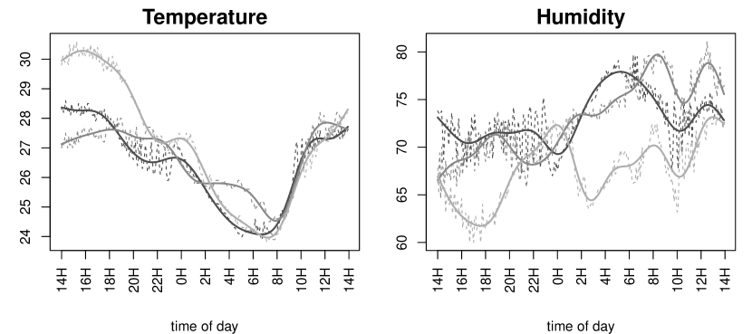
Figure 1: Temperature (^∘C) and humidity ($\%$) observed profiles (dashed) for three randomly selected days and the corresponding smoothed ones (solid); the x-axis begins at 14H (2PM).

For the analysis we smooth daily temperature measurements of each sow using univariate smoother with $15$ cubic regression bases and quadratic penalty; REML is used to estimate smoothing parameter. The smoothed temperature curve for sow $i$’s $j$th repeated measure is denoted by $T_{ij}(t)$, $t\in[0,24)$, and the corresponding daily average humidity is denoted by $AH_{ij}$. Both temperature and average humidity are centered before being used in the analysis.

For convenience we denote the response with $\Delta_{ij}$ by removing the superscript. In this application for fixed $j$, $\Delta_{ij}$ corresponds to $Y_{i}$ in Section 2, $P_{i}$ and $AH_{ij}$ correspond to scalar covariates $X_{i2}$, and $T_{ij}(t)$ and $AH_{ij}\cdot T_{ij}(t)$ to functional covariates $X_{i3}(\cdot)$. We first estimate the conditional distribution of $\Delta_{ij}$ given temperature $T_{ij}(t)$, average humidity $AH_{ij}$, parity $P_{i}$, and interaction $AH_{ij}\cdot T_{ij}(t)$. Specifically for each of lactation days of interest ($j=3,10$ and $17$) we create a set of $100$ equi-spaced grid of points between the fifth smallest and fifth largest values of $\Delta_{ij}$’s and denote the grids with $\mathcal{D}=\{d_{\ell}:\ell=1,\ldots,100\}$. Then we create artificial binary responses, $\{\mathbbm{1}\left(\Delta_{ij}\leq d_{\ell}\right):\ell=1,\ldots,100\}$, and fit the following model for $F_{ij}(d_{\ell})=E\left[\mathbbm{1}\left(\Delta_{ij}\leq d_{\ell}\right)\big{|}T_{ij}(t),AH_{ij},P_{i}\right]$:

$$E\left[\mathbbm{1}\left(\Delta_{ij}\leq d_{\ell}\right)\big{|}T_{ij}(t),AH_{ij},P_{i}\right]=g^{-1}\Big{\{}\beta_{0}(d_{\ell})+\beta_{1}(d_{\ell})P_{i}+\beta_{2}(d_{\ell})AH_{ij}$$

$$+\int\beta_{3}(d_{\ell},t)T_{ij}(t)dt+AH_{ij}\int\beta_{4}(d_{\ell},t)T_{ij}(t)dt\Big{\}},$$

where $\beta_{0}(\cdot)$ is a smooth intercept, $\beta_{1}(\cdot)$ quantifies the smooth effect of young sows, $\beta_{2}(\cdot)$ describes the effect of the humidity, and $\beta_{3}(\cdot,t)$ and $\beta_{4}(\cdot,t)$ quantify the effect of the temperature at time $t$ as well as the interaction between the temperature at time $t$ and average humidity. We model $\beta_{0}(\cdot)$ using 20 univariate basis functions, $\beta_{1}(\cdot)$ and $\beta_{2}(\cdot)$ using five univariate basis functions, $\beta_{3}(\cdot,\cdot)$ and $\beta_{4}(\cdot,\cdot)$ using tensor product of two univariate bases functions (total of 25 functions). Throughout the analysis, cubic B-spline bases are used and REML is used for estimating smoothing parameters. The estimated conditional distribution, denoted by $\widehat{F}_{ij}(d)$, is monotonized by fitting isotonic regression to $\{(d_{\ell},\widehat{F}_{ij}(d_{\ell})):\ell=10,\ldots,90\}$ ; ten smallest and ten largest $d_{\ell}$ and the corresponding values of $\widehat{F}_{j}(d_{\ell})$ are removed to avoid boundary effects. By abuse of notation, $\widehat{F}_{ij}(d)$ denotes the resulting monotonized estimated distribution. Finally, we obtain estimated first quartiles, i.e. quantiles at $\tau=0.25$ level, by inverting $\widehat{F}_{ij}(d)$, namely $\widehat{Q}\left(\tau=0.25\;|\;T_{ij}(t),AH_{ij},P_{i}\right)=\text{inf}\{d:\widehat{F}_{ij}(d)\geq 0.25\}$.

To understand the relationship between the lactating sows feed intake and the thermal condition of the farrowing room, we systematically compare and study the predicted quantiles of two responses at combinations of different values of temperature, humidity, and parity. For each of three lactation days ($j=3,10,17$) we consider three values of average humidity (first quartile, median, and third quartile) and two levels of parity ($0$ for older sows and $1$ for younger sows). Based on the experimenters’ interest, for the functional covariate $T_{ij}(\cdot)$ we consider seven smooth temperature curves given in Figure 2. Each of these curves are obtained by first calculating pointwise quantiles of temperature at five-minute intervals for a specific level and then smoothing it; we considered quantiles levels $\eta=0.2,0.3,\ldots,$ and $0.8$. In short, for each of three lactation days we obtain the first quartile of two responses for 42 different combinations ($3$ humidity values $\times$ 2 parity levels $\times$ 7 temperature curves) using the proposed method. To avoid extrapolation we ascertain that (i) there are reasonably many observed measurements at each of the combinations and (ii) bottom 25% of the responses are not dominantly from one of the parity group; see distribution of each response by the parity in Figure 3.

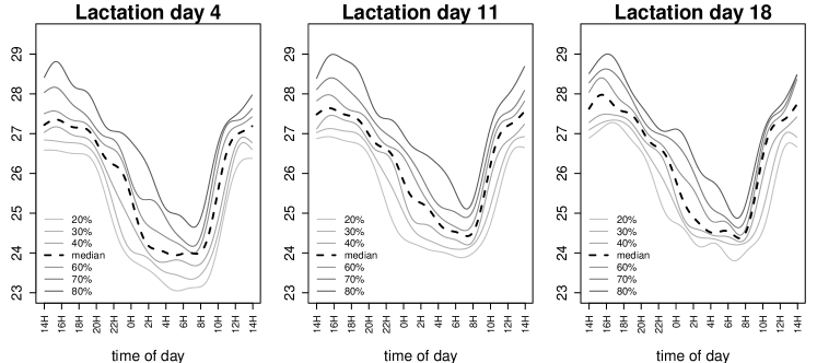
Figure 2: Temperature curves with which prediction of quantiles is made. Dashed black line is pointwise average of temperature curves and solid lines are pointwise quartiles; all curves are smoothed.

Figure 3: Top panels: back-to-back boxplots of the absolute change in feed intake at a specific day by parity; Bottom panels: back-to-back boxplots of the relative change in feed intake at a specific day by parity.

The resulting predicted quantiles are shown in Figure 4. Here we focus our discussion on predicted quantile of $\Delta^{(2)}_{i(j+1)}$ at quantile level $\tau=0.25$ for lactation day 4 ($j=3$) - the first plot of the second row in Figure 4. The results suggest that the feed intake of older sows (parity $P_{i}=0$; grey lines) are less affected by high temperatures than younger sows (black lines); this finding is in agreement with Bloemhof et al., (2013). We also observe that the effects of humidity and temperature on feed intake change are strongly intertwined. For illustration, we focus on lactation day 4 ($j=3$) again for younger sows (black lines). For medium humidity (dashed lines) their feed intake stays pretty constant as temperature increases, while for low and high humidity levels (solid and dotted lines, respectively) it changes with an opposite direction. Specifically when temperature increases the predicted first quartile of $\Delta^{(2)}_{i(j+1)}$ increases for low humidity (solid line) whereas it decreases for high humidity (dotted line). Our results imply that high humidity (dotted line) is related to a negative impact of high temperature on feed intake while low humidity (solid line) alleviates it; and this finding is consistent with a previous study (Bergsma and Hermesch,, 2012). The analysis result suggests to keep low humidity levels in order to maintain healthy feed intake behavior, when ambient temperature is above $60$th percentile; high humidity levels are desirable for cooler ambient temperature.

Interpretation of the other results is similar. While the effects of covariates on feed intake are less apparent toward the end of lactation period, we still observe similar pattern across all three lactation days. For the 11th day ($j=10$), the 25th quantile of the feed intake is predicted to decrease when the temperature stays below the $40$th percentile, regardless of humidity level and sows age. However, it starts increasing with low humidity while it continues decreasing with high humidity when the temperature rises above the $40$th percentile. Similarly, for the 18th day ($j=17$) when the temperature rises above the $60$th percentile, the predicted first quartile increases with low humidity while it decreases with high humidity. The effect of temperature on feed intake seems less obvious for lactation days 11 and 18 than for day 4; while the effect may be due to lactation day, it may also be a result of other factors, such as more fluctuation and variability in temperature curves on day 4 than on other two days (see Figure 2). Overall we conclude that high humidity and temperature affect the sows feed intake behavior negatively and young sows (parity one) are more sensitive to heat stress than older sows (higher parity), especially at the beginning of lactation period.

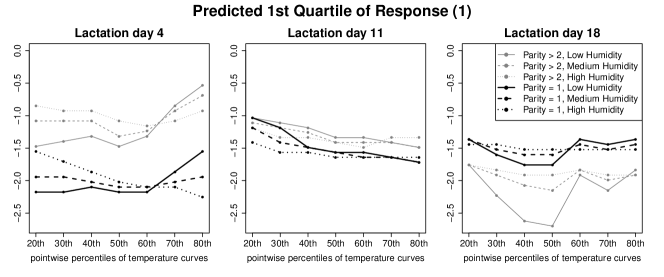
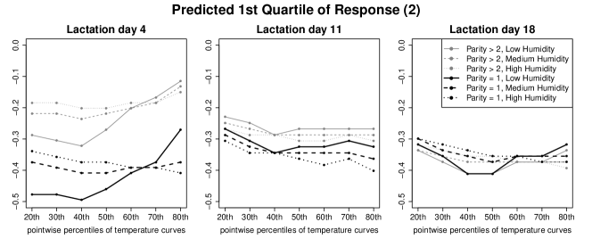
Figure 4: Displayed are the predicted quantiles of $\Delta^{(1)}_{i(j+1)}$ and $\Delta^{(2)}_{i(j+1)}$ for different parities, average humidity, and temperature levels. In each of all six panels, black thick lines correspond to the young sows ($P_{i}=1$) and grey thin lines correspond to the old sows ($P_{i}=0$). Line types indicate different average humidity levels; solid, dashed, and dotted correspond to low, medium, and high average humidity levels (given by the first quartile, median, and the third quartiles of $AH_{ij}$), respectively. The seven grids in $x$-axis of each panel correspond to the $7$ temperature curves given in the respective panel of Figure 2.

6 Discussion

The proposed modeling framework opens up a couple of future research directions. A first research avenue is to develop significance tests of null covariate effect. Testing for the null effect of a covariate on the conditional distribution of the response is equivalent to testing that the corresponding regression coefficient function is equal to zero in the associated function-on-function mean regression model. Such significance tests have been studied when the functional response is continuous (Shen and Faraway,, 2004; Zhang and Chen,, 2007); however their study for binary-valued functional responses is an open problem in functional data literature, and only recently has been considered in Chen et al., (2018). Another research avenue is to do variable selection in the setting where there are many scalar covariates and functional covariates. Many current applications collect data with increasing number of mixed covariates and selecting the ones that have an effect on the conditional distribution of the response is very important. This problem is an active research area in functional mean regression where the response is normal (Gertheiss et al.,, 2013; Chen et al.,, 2016). The proposed modeling framework has the potential to facilitate studying such problem.

Data Availability

The data used to support the findings of this study are available from the corresponding author upon request.

Conflicts of Interest

The authors declare that they have no conflicts of interests.

Funding Statement

Staicu’s research was supported by National Science Foundation DMS 0454942 and DMS 1454942, and National Institutes of Health grants R01 NS085211, R01 MH086633, 5P01 CA142538-09.

Supplementary materials

Section LABEL:sec:_sim-add provides additional simulation settings and results for the cases of having either a single scalar covariate or a single functional covariate. Additional results for the case of having a scalar covariate and a densely observed functional covariate are also included. Section LABEL:sec:_bike_sharing presents additional data analysis using the proposed method on the bike sharing dataset (Fanaee-T and Gama,, 2014; Lichman,, 2013).

References

- Barlow, (1972) Barlow, R. E. (1972). Statistical inference under order restrictions; the theory and application of isotonic regression. Technical report.
- Bergsma and Hermesch, (2012) Bergsma, R. and Hermesch, S. (2012). Exploring breeding opportunities for reduced thermal sensitivity of feed intake in the lactating sow. Journal of animal science, 90(1):85–98.
- Black et al., (1993) Black, J., Mullan, B., Lorschy, M., and Giles, L. (1993). Lactation in the sow during heat stress. Livestock production science, 35(1):153–170.
- Bloemhof et al., (2013) Bloemhof, S., Mathur, P., Knol, E., and Van der Waaij, E. (2013). Effect of daily environmental temperature on farrowing rate and total born in dam line sows. Journal of animal science, 91(6):2667–2679.
- Bondell et al., (2010) Bondell, H., Reich, B., and Wang, H. (2010). Noncrossing quantile regression curve estimation. Biometrika, 97(4):825–838.
- Cardot et al., (2005) Cardot, H., Crambes, C., and Sarda, P. (2005). Quantile regression when the covariates are functions. Nonparametric Statistics, 17(7):841–856.
- Cardot et al., (1999) Cardot, H., Ferraty, F., and Sarda, P. (1999). Functional linear model. Statistics & Probability Letters, 45(1):11–22.
- Chen and Müller, (2012) Chen, K. and Müller, H.-G. (2012). Conditional quantile analysis when covariates are functions, with application to growth data. Journal of the Royal Statistical Society: Series B (Statistical Methodology), 74(1):67–89.
- Chen et al., (2018) Chen, S., Xiao, L., and Staicu, A.-M. (2018). Testing for generalized scalar-on-function linear models. Submitted.
- Chen et al., (2016) Chen, Y., Goldsmith, J., and Ogden, R. T. (2016). Variable selection in function-on-scalar regression. Stat, 5(1):88–101.
- Chernozhukov et al., (2009) Chernozhukov, V., Fernandez-Val, I., and Galichon, A. (2009). Improving point and interval estimators of monotone functions by rearrangement. Biometrika, 96(3):559–575.
- Eilers and Marx, (1996) Eilers, P. H. and Marx, B. D. (1996). Flexible smoothing with b-splines and penalties. Statistical science, pages 89–102.
- Fanaee-T and Gama, (2014) Fanaee-T, H. and Gama, J. (2014). Event labeling combining ensemble detectors and background knowledge. Progress in Artificial Intelligence, 2(2-3):113–127.
- Ferraty et al., (2005) Ferraty, F., Rabhi, A., and Vieu, P. (2005). Conditional quantiles for dependent functional data with application to the climatic “el niño” phenomenon. Sankhyā: The Indian Journal of Statistics, pages 378–398.
- Ferraty and Vieu, (2006) Ferraty, F. and Vieu, P. (2006). Nonparametric Functional Data Analysis. Springer, New York.
- Ferraty and Vieu, (2009) Ferraty, F. and Vieu, P. (2009). Additive prediction and boosting for functional data. Computational Statistics & Data Analysis, 53(4):1400–1413.
- Gertheiss et al., (2013) Gertheiss, J., Maity, A., and Staicu, A.-M. (2013). Variable selection in generalized functional linear models. Stat, 2(1):86–101.
- Goldsmith et al., (2011) Goldsmith, J., Bobb, J., Crainiceanu, C. M., Caffo, B., and Reich, D. (2011). Penalized functional regression. Journal of Computational and Graphical Statistics, 20(4):830–851.
- Huang et al., (2015) Huang, L., Scheipl, F., Goldsmith, J., Gellar, J., Harezlak, J., Mclean, M., Swihart, B., Xiao, L., Crainiceanu, C., Reiss, P., Chen, Y., Greven, S., Huo, L., Kundu, M., and Wrobel, J. (2015). R package refund: Methodology for regression with functional data (version 0.1-13). URL: https://cran.r-project.org/web/packages/refund/index.html.
- Ivanescu et al., (2015) Ivanescu, A. E., Staicu, A.-M., Scheipl, F., and Greven, S. (2015). Penalized function-on-function regression. Computational Statistics, 30(2):539–568.
- James, (2002) James, G. M. (2002). Generalized linear models with functional predictors. Journal of the Royal Statistical Society: Series B (Statistical Methodology), 64(3):411–432.
- Johnston et al., (1999) Johnston, L., Ellis, M., Libal, G., Mayrose, V., and Weldon, W. (1999). Effect of room temperature and dietary amino acid concentration on performance of lactating sows. ncr-89 committee on swine management. Journal of animal science, 77(7):1638–1644.
- Kato, (2012) Kato, K. (2012). Estimation in functional linear quantile regression. The Annals of Statistics, 40(6):3108–3136.
- Kim et al., (2018) Kim, J. S., Staicu, A.-M., Maity, A., Carroll, R. J., and Ruppert, D. (2018). Additive function-on-function regression. Journal of Computational and Graphical Statistics, 27(1):234–244.
- Koenker, (2005) Koenker, R. (2005). Quantile Regression. Number 38. Cambridge university press.
- Koenker and Bassett Jr, (1978) Koenker, R. and Bassett Jr, G. (1978). Regression quantiles. Econometrica: journal of the Econometric Society, pages 33–50.
- Lichman, (2013) Lichman, M. (2013). UCI machine learning repository.
- Lu et al., (2014) Lu, Y., Du, J., and Sun, Z. (2014). Functional partially linear quantile regression model. Metrika, 77(2):317–332.
- McLean et al., (2014) McLean, M. W., Hooker, G., Staicu, A.-M., Scheipl, F., and Ruppert, D. (2014). Functional generalized additive models. Journal of Computational and Graphical Statistics, 23(1):249–269.
- Melillo, (2014) Melillo, J. M. (2014). Climate change impacts in the united states, highlights: Us national climate assessment.
- Nelson et al., (2009) Nelson, G. C., Rosegrant, M. W., Koo, J., Robertson, R., Sulser, T., Zhu, T., Ringler, C., Msangi, S., Palazzo, A., Batka, M., et al. (2009). Climate Change: Impact on Agriculture and Costs of Adaptation, volume 21. Intl Food Policy Res Inst.
- Ng and Maechler, (2007) Ng, P. and Maechler, M. (2007). A fast and efficient implementation of qualitatively constrained quantile smoothing splines. Statistical Modelling, 7(4):315–328.
- Quiniou and Noblet, (1999) Quiniou, N. and Noblet, J. (1999). Influence of high ambient temperatures on performance of multiparous lactating sows. Journal of animal science, 77(8):2124–2134.
- Ramsay and Silverman, (2005) Ramsay, J. and Silverman, B. (2005). Functional Data Analysis. Springer, New York.
- Ramsay and Silverman, (2002) Ramsay, J. and Silverman, B. W. (2002). Applied Functional Data Analysis: Methods and Case Studies. Springer, New York.
- Renaudeau and Noblet, (2001) Renaudeau, D. and Noblet, J. (2001). Effects of exposure to high ambient temperature and dietary protein level on sow milk production and performance of piglets. Journal of animal science, 79(6):1540–1548.
- Renaudeau et al., (2001) Renaudeau, D., Quiniou, N., and Noblet, J. (2001). Effects of exposure to high ambient temperature and dietary protein level on performance of multiparous lactating sows. Journal of Animal Science, 79(5):1240–1249.
- Rosero et al., (2016) Rosero, D. S., Boyd, R. D., McCulley, M., Odle, J., and van Heugten, E. (2016). Essential fatty acid supplementation during lactation is required to maximize the subsequent reproductive performance of the modern sow. Animal Reproduction Science, 168:151–163.
- Ruppert, (2002) Ruppert, D. (2002). Selecting the number of knots for penalized splines. Journal of computational and graphical statistics, 11(4):735–757.
- Scheipl et al., (2016) Scheipl, F., Gertheiss, J., Greven, S., et al. (2016). Generalized functional additive mixed models. Electronic Journal of Statistics, 10(1):1455–1492.
- Shen and Faraway, (2004) Shen, Q. and Faraway, J. (2004). An f test for linear models with functional responses. Statistica Sinica, pages 1239–1257.
- St-Pierre et al., (2003) St-Pierre, N., Cobanov, B., and Schnitkey, G. (2003). Economic losses from heat stress by us livestock industries. Journal of dairy science, 86:E52–E77.
- Tang and Cheng, (2014) Tang, Q. and Cheng, L. (2014). Partial functional linear quantile regression. Science China Mathematics, 57(12):2589–2608.
- Wood, (2006) Wood, S. (2006). Generalized Additive Models: An Introduction with R. Chapman and Hall/CRC.
- Wood, (2003) Wood, S. N. (2003). Thin plate regression splines. Journal of the Royal Statistical Society: Series B (Statistical Methodology), 65(1):95–114.
- (46) Xiao, L., Li, C., Checkley, W., and Crainiceanu, C. (2018a). Fast covariance estimation for sparse functional data. Statistics and computing, 28(3):511–522.
- (47) Xiao, L., Li, C., Checkley, W., and Crainiceanu, C. (2018b). R package face: Fast covariance estimation for sparse functional data (version 0.1-4). URL:http://cran.r-project.org/web/packages/face/index.html.
- Xiao et al., (2016) Xiao, L., Zipunnikov, V., Ruppert, D., and Crainiceanu, C. (2016). Fast covariance estimation for high-dimensional functional data. Statistics and Computing, 26(1-2):409–421.
- Yao et al., (2005) Yao, F., Müller, H.-G., and Wang, J.-L. (2005). Functional data analysis for sparse longitudinal data. Journal of the American Statistical Association, 100(470):577–590.
- Yu et al., (2016) Yu, D., Kong, L., and Mizera, I. (2016). Partial functional linear quantile regression for neuroimaging data analysis. Neurocomputing, 195:74–87.
- Zhang and Chen, (2007) Zhang, J.-T. and Chen, J. (2007). Statistical inferences for functional data. The Annals of Statistics, 35(3):1052–1079.