Distributed Parallel D8 Up-Slope Area Calculation in Digital Elevation Models

Abstract

This paper presents a parallel algorithm for calculating the eight-directional (D8) up-slope contributing area in digital elevation models. In contrast with previous algorithms, which have potentially unbounded inter-node communications, the algorithm presented here realizes strict bounds on the number of inter-node communications. Those bounds in turn allow D8 attributes to be processed for arbitrarily large DEMs on hardware ranging from average desktops to supercomputers. The algorithm can use the OpenMP and MPI parallel computing models, either in combination or separately. It partitions the DEM between slave nodes, calculates an internal up-slope area by replacing information from other slaves with variables representing unknown quantities, passes the results on to a master node which combines all the slaves’ data, and passes information back to each slave, which then computes its final result. In this way each slave’s DEM partition is treated as a simple unit in the DEM as a whole and only two communications take place per node.

Keywords: D8, up-slope area, digital elevation model, distributed, parallel, flow accumulation

1 Introduction

DEMs are data structures, usually a rectangular array of floating-point or integer values, representing terrain elevation above some common base level, generally measured via remote sensing techniques or LIDAR.

DEMs are used extensively to model hydrologic processes and properties including soil moisture (based on catchment area), terrain instability (based on slope and catchment area), erosion (based on slope), and stream power (based on slope and catchment area) [5].

Underlying the aforementioned calculations is a flow function responsible for determining what proportion of each cell’s flow each neighbouring cell will receive. Perhaps the most widely used function is the D₈ function introduced by O’Callaghan and Mark [3]. This function directs the entirety of each cell’s flow to the lowest of its eight surrounding neighbours. This implies that flows combine but never disperse: a property we take advantage of. In contrast is the D_∞ method introduced by Tarboton [4], which calculates an angle of steepest descent based on adjacent pairs of neighbouring cells and directs flow to one or both neighbours along that path.

The accuracy of DEM-based calculations is related to the DEM’s resolution. These have gone from thirty-plus meter resolution in the recent past to the sub-meter resolutions becoming available today. Increasing resolution has led to increased data sizes: current data sets are on the order of gigabytes and increasing. While computer processing and memory performance have increased appreciably during this time, legacy equipment and algorithms suited to manipulating smaller DEMs with coarser resolutions make processing these improved data sources costly, if not impossible.

Wallis et al. [5] present one solution for calculating “up-slope area" based on previous work by Mark [2] and O’Callaghan and Mark [3]: a parallel algorithm suitable for both D₈ and D_∞ calculations for use in environments where communication is inexpensive using a queue-based up-slope area function. Although their algorithm, as published, assumes shared memory, this is not a strict requirement.

The algorithm presented here applies only to D₈, is suitable for environments where inter-node communication is expensive relative processing, makes efficient use of multi-processor nodes, and optimises the queue method presented by Wallis et al. [5].

2 Up-Slope Area

Up-slope area $A$ is defined physically for each point $p$ in a watershed as the set of all points $P$ whose flow, if we were to put a liquid in them, would eventually pass through $p$. Mathematically, this is defined by the recursion relation:

$$A(p)=1+\sum_{i=n(p,P)}A(i)$$ (1)

Where $n(p,P)$ defines the points neighbouring $p$, given $P$. In practice, points are generally represented by cells of some sort, which may or may not be of equal area and may or may not be weighted equally in the calculation. In the case of most DEMs and this paper, the points are represented by square cells with an area and weight of one.

3 The Algorithm

It is assumed that the DEM has been preprocessed to remove pits and flats. Pits are cells with no lower neighours or groups of cells from which there is no outlet. In the case of a single cell, the cell is generally raised to the level of its lowest neighbor; in the case of groups, an outlet is usually drilled. Flats are cells with one or more neighbours of equal elevation, these my be resolved by making slight elevation modifications within the flat; Garbrecht and Martz [1] present one approach.

Following this, each of $S$ slave nodes reads in an equal number of horizontal rows of the DEM, with any extra rows allocated to the final slave. In addition to its allotted rows, each slave also reads in two extra rows above and below its strip. This permits the slave to determine flow direction for the cells at the edge of its allotted strip and for the cells bordering it. Henceforth, cells at the edge of a slave’s allotted strip are called edge cells and are found in either the $TopRow$ or the $BottomRow$ of the strip.

In this algorithm, the D₈ flow direction of a cell is specified as being towards the neighbour with the steepest slope relative that cell using the Euclidean distance between centers of the two cells. We call the net flow field $F$.

Throughout this paper procedures marked with a parallel subscript (“_∥") may be safely invoked on multiple processors whereas loops marked with a parallel subscript be safely partitioned between processors. Any commands which may lead to race conditions are marked as atomic.

Using the flow field $F$, each slave finds the dependencies of all its cells using Algorithm 1. A cell $c$ is a dependent of a neighbour $n$ if $n$’s flow is directed into it; thus, a cell may have 0–8 dependencies, inclusive. If a cell has no dependencies, it is pushed on to the back of a double-ended queue $Q$; otherwise, the number of dependencies is stored in an array $D$.

Algorithm 1 Slaves calculate dependencies

1:procedure FindDependencies

2:$F,D,Q$

3:     for_∥ all $c$ in $F$

4:         for all $n$ inputs to $c$ do

5:              $D(c)\leftarrow D(c)+1$

6:         end for

7:         if $D(c)=0$ then

8:              Atomic(push $c$ onto back of $Q$)

9:         end if

10:     end for_∥

11:end procedure

The purpose of the double-ended queue is to minimize contention in multi-processor environments by decoupling the queue’s push and pop functions. The for_∥ loop on Line 3 may be safely run in parallel because none of the data being read is altered by the function and only one processor will be writing to any given memory location. The queue-push on Line 8 must be done atomically for the algorithm to run safely. It is possible to implement Algorithm 1 such that there is no contention by having each processor build its own queue and then merging these just after the function completes.

Following Algorithm 1, each slave performs calculates its Internal Up-slope Area $A$ using Algorithm 2. This algorithm begins with the local maxima of the DEM—those cells added to $Q$ by Algorithm 1—which have an up-slope area of one (only themselves) and decrements the dependency counter of the cells they flow into. When a cell’s dependency counter reaches zero, it is added to $Q$. Thus, as the up-slope area of higher-elevation cells becomes known, it is possible to calculate that of lower-elevation cells.

Algorithm 2 Slaves calculate internal up-slope area

1:procedure InternalUpslope_∥($c$)

2:$F,D,Q,A$

3:     if $c$ was not specified then

4:         Atomic($c\leftarrow$ front of $Q$)

5:         if $c$ was not set then

6:              return

7:         end if

8:     end if

9:

10:     $A(c)\leftarrow 1$

11:     for all $n$ inputs to $c$ do

12:         $A(c)\leftarrow A(c)+A(n)$

13:     end for

14:

15:     $n\leftarrow$ downslope neighbor of $c$

16:     if $n$ exists then

17:         $D(n)\leftarrow D(n)-1$

18:         if $D(n)\neq 0$ then

19:              $n\leftarrow$NULL

20:         end if

21:     end if

22:     return InternalUpslope($n$)

23:end procedure

Algorithm 2 is defined using tail recursion and, to avoid excessive stack sizes, should be implemented appropriately. Since $Q$ cannot be equitably divided among processors beforehand, it is necessary for each processor to atomically pop cells from it when necessary. However, the depth-first search embodied by the recursion on Line 22 reduces contention on $Q$.

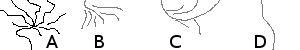
Figure 1: Conceptual image of dependencies and resolutions

At this point, information from other slaves is required to resolve the remaining dependencies. Figure 1 depicts this conceptually. A represents a flow path originating in the current slave’s portion of the DEM: all its dependencies can be satisfied with the information available to the slave, but these results must be communicated to neighbouring slaves.

If we assume that flow is generally directed to the lower-right, then B represents an up-slope area originating in a different slave and terminating in this one. In such a case a single communication between the slaves provides sufficient information to compute up-slope area.

C represents a similar situation, but two communications are necessary because the flow path loops back up: one to resolve this slave’s dependencies and another to resolve its neighbour’s.

D represents a situation in which two communications are necessary to pass information from one neighbouring slave to another through the current slave.

If C and D link through the upper neighbouring slave, then four communications would be necessary. Or, if flow is directed to the upper-left, and B, C, and D are linked, then five communications would be necessary. We denote the average number of communications a slave will need to make as its “winding factor" $\phi$. In situations where communication is cheap, $\phi$ is unimportant and algorithms such as that presented by Wallis et al. [5] are effective. In situations where communication is expensive, a different algorithm, such as that presented here, is necessary.

If each slave denotes external inputs from other slaves by variables, it is possible to continue the calculation with minimally inter-nod communication.

We call edge cells with unresolved dependencies in other slaves’ DEMs receivers. They receive information from at most 3 of the other slave’s edge cells. Cells upon which another slave’s DEM depends are either givers or joiners. A giver cell’s upslope-area has already been calculated by Algorithm 2; a joiner is the dependent of one or more receiver cells.

It is a property of the D₈ flow function that flows join but never disperse and, therefore, that every joiner is a dependent of at least one receiver while each receiver ultimately feeds into at most one joiner. This property does not hold for the D_∞ flow function, preventing its use in this context.

Algorithm 3 presents one possible way of preparing the slave to perform the External Up-slope Area calculation. The original dependency grid is saved on Line 3 to be used later in calculating the true up-slope area. Once this is done, the external dependencies of all edge cells are removed and those cells which are “satisfied" are added to $Q$. The cell is marked as a receiver by assigning it a special variable name on Line 6.

$Cell_{V}$, first mentioned on Line 6, is a map between cells $c$ and variable names, which are represented as globally-unique numbers with $-1$ acting as a special value used to denote receivers. Algorithm 3 marks all cells as receivers; Algorithm 4 will remark those which are not.

Algorithm 3 Slaves prepare to calculate external up-slope area

1:procedure SatisfyReceivers

2:$F,D,D_{O},Cell_{V},Q$

3:     $D_{O}\leftarrow D$

4:     for_∥ all $c$ in $TopRow$

5:         $V\leftarrow$NewVariable

6:         $Cell_{V}(c)\leftarrow-1$

7:         for all $n$ above-inputs to $c$ do

8:              $D(c)\leftarrow D(c)-1$

9:         end for

10:         if $D(c)=0$ then

11:              Atomic(push $c$ onto back of $Q$)

12:         end if

13:     end for_∥

14:     $\triangleright$ Analogous code for $BottomRow$

15:end procedure

Algorithm 4 calculates External Up-slope Area, keeping track of how cells depend on receivers. When a cell is popped off $Q$, it is associated with a new variable name $V$ (Line 8) which is unique across all slaves and used in future iterations to keep track of the flow path’s origin using the multimap $Origin$ (Line 9). Since only edge cells are in $Q$, new variables are only formed at the edge cells.

After incrementing a cell $c$’s up-slope area, the algorithm attempts to follow the flow path from $c$ to its neighbour $n$ (Line 23). If there is a neighbour and its dependencies are satisfied, the algorithm recurses, maintaining knowledge of which edge cell its flow path originated at using $V$ (Line 27). If $n$’s dependencies are not satisfied, the algorithm uses the map $Cell_{V}$ to inform a future iteration of the existence of the flow path it’s about to abandon (Line 30).

On Lines 17–21, after the cell’s up-slope area has been incremented, the algorithm inspects the present cell and and cells flowing into it to see if it or they are part of a previously abandoned flow path. If so, it merges that flow path with the present one and continues.

Algorithm 4 Slaves calculate external up-slope area

1:procedure ExternalUpslope_∥($V,c$)

2:$F,D,Q,A,Cell_{V},Origin$

3:     if $c$ was not specified then

4:         Atomic($c\leftarrow$ front of $Q$)

5:         if $c$ was not set then

6:              return

7:         end if

8:         $V\leftarrow$NewVariable

9:         $Origin(V)\leftarrow c$

10:     end if

11:

12:     $A(c)\leftarrow 1$

13:     for all $n$ inputs to $c$ do

14:         $A(c)\leftarrow A(c)+A(n)$

15:     end for

16:

17:     for all $n$ inputs to $c$ and $c$ itself do

18:         append $Origin(Cell_{V}(n))$ to $Origin(V)$

19:         erase $Origin(Cell_{V}(n))$

20:         erase $Cell_{V}(n)$

21:     end for

22:

23:     $n\leftarrow$ downslope neighbor of $c$

24:     if $n$ exists then

25:         $D(n)\leftarrow D(n)-1$

26:         if $D(n)=0$ then

27:              return ExternalUpslope($V,n$)

28:         end if

29:     end if

30:     $Cell_{V}(c)=V$

31:     return ExternalUpslope($-,-$)

32:end procedure

Ultimately, the algorithm reaches a point where no down-slope neighbour exists and there are no more cells in $Q$. It abandons the flow path (Line 30), recurses, and exits (Line 6). The result of this algorithm is a map $Cell_{V}$ indexed on the joiner cells. These cells are part of the border of the current slave and the edge of the adjacent slave—they are the adjacent slave’s receivers. So $Cell_{V}$, coupled with $Origin$ link one slave’s receivers to another’s.

Each slave now sends $Cell_{V}$, $Origin$, and the up-slope area of its bordering cells to the master node.

Conceptually, the situation is exemplified by Figure 2. Data from different slaves is separated by wide vertical gaps; it is important to remember that the cells bordering these gaps, though they appear in different slaves are, in fact, the same in the DEM. Within a slave’s data, receivers and joiners form sometimes-complicated linkages while between slaves the linkages are simple; from the master’s perspective, the slaves combine to form a directed acyclic graph.

Figure 2: Conceptual image of master node’s data

In Figure 2, receivers are marked by variables. These are passed along to joiners, accumulating up-slope area along the way. Therefore, the joiners are represented by the sum of their associated receivers’ variables and the upslope area connecting them to each receiver. Givers are represented by a pure number: this is a true up-slope area and a starting point for the next calculation.

Algorithm 5 prepares the slaves’ data for processing by locating giver cells and determining how many dependencies each joiner has. Since the map keys are globally unique, all the slaves’ $Cell_{V}$s are combined; likewise, the $Origin$s. The function Invert on Line 16 turns $Origin$’s keys into values and vice versa. The result is a simple map serving the same purpose as the flow field array $F$ of Algorithm 2. The dependency array holds: 1 for receivers since they only depend on data from cells in adjacent slaves; -1 for givers so that they are not later mistaken for receivers; and a positive number, 1 or more, for joiners.

Algorithm 5 Master node prepares received data

1:procedure MasterPrep

2:$D,Q,Cell_{V},Origin$

3:     for_∥ all Slaves $s$

4:         for all $c$ in $(TopRow,BottomRow)$ do

5:              if $Cell_{V}(c)$ is undefined then $\triangleright$ Giver

6:                  Atomic(push $c$ onto back of $Q$)

7:                  $D(c)\leftarrow-1$

8:              else if $Cell_{V}(c)=-1$ then

9:$\triangleright$ Receiver

10:                  $D(c)\leftarrow 1$

11:              else$\triangleright$ Joiner

12:                  $D(c)\leftarrow$Length($Origin(Cell_{V}(C))$)

13:              end if

14:         end for

15:     end for_∥

16:     $Destination\leftarrow$Invert($Origin$)

17:end procedure

Algorithm 6 solves the system of equations presented by the slaves using the same methodology as in Algorithms 2 and 4. Lines 10–20 identify the cell’s destination. If one has not been explicitly declared the cell must either be a giver or a joiner and its destination is implied as being to the slave above/below it, provided that cell is a receiver. Figure 2 depicts one situation wherein this would arise. The destination of the cell in the bottom right labeled “$c+9$" is implied to be directly below it; however, the two are unconnected. If the destination is valid, the algorithm continues in the usual fashion.

Algorithm 6 Master node calculates up-slope area

1:procedure MasterUpslope_∥($c$)

2:$A,D,Q,Cell_{V},Destination$

3:     if $c$ was not specified then

4:         Atomic($c\leftarrow$ front of $Q$)

5:         if $c$ was not set then

6:              return

7:         end if

8:     end if

9:

10:     $n\leftarrow Destination(c)$

11:     if $n$ is undefined then

12:         if $c$ is a top cell then

13:              $n\leftarrow$cell above $c$

14:         else

15:              $n\leftarrow$cell below $c$

16:         end if

17:         if $Cell_{V}(n)\neq-1$ then$\triangleright$ Not A Receiver

18:              $n\leftarrow$NULL

19:         end if

20:     end if

21:     if $n$ is undefined then

22:         return MasterUpslope($-$)

23:     end if

24:

25:     $A(n)\leftarrow A(n)+A(c)$

26:     $D(n)\leftarrow D(n)-1$

27:     if $D(n)\neq 0$ then

28:         $n\leftarrow$NULL

29:     end if

30:     return MasterUpslope($n$)

31:end procedure

Algorithm 7 Slaves prepare incoming data

1:procedure PrepFinaliseInternal

2:$F,D,D_{O},Cell_{V},Q$

3:     $D\leftarrow D_{O}$

4:     for_∥ all $c$ in $TopRow$

5:         for all $n$ above-inputs to $c$ do

6:              $D(c)\leftarrow D(c)-1$

7:         end for

8:         if $D(c)=0$ then

9:              Atomic(push $c$ onto back of $Q$)

10:              $Area_{D}(c)\leftarrow A_{incoming}(c)$

11:         end if

12:     end for_∥

13:     $\triangleright$ Analogous code for $BottomRow$

14:end procedure

Once Algorithm 6 is completed, the area of each slaves’ top and bottom rows are returned. Since Algorithm 4 set the areas of the slaves’ receivers to one and calculated up-slope area that, we simply have to add each receivers’ incoming area to all its dependents. Line 10 of Algorithm 7 enables this by setting up a map between receivers and their incoming variables. This map will later be used to keep track of which incoming areas belong to which flow path. Finally, the slaves run Algorithm 8.

Algorithm 8 is similar to Algorithm 4 insofar as it propagates variables forward. However, rather than propagating variables and combining flow paths, only the incoming areas are propagated forward.

Algorithm 8 Slaves finalise internal up-slope areas

1:procedure FinaliseInternal_∥($S,c$)

2:$F,D,Q,A$

3:     if $c$ was not specified then

4:         Atomic($c\leftarrow$ front of $Q$)

5:         if $c$ was not set then

6:              return

7:         end if

8:         $S\leftarrow Area_{D}(c)$

9:     end if

10:

11:     for all $n$ inputs to $c$ do

12:         $S\leftarrow S+Area_{D}(c)$

13:         erase $Area_{D}(c)$

14:     end for

15:     $A(c)\leftarrow A(c)+S$

16:

17:     $n\leftarrow$ downslope neighbor of $c$

18:     if $n$ exists then

19:         $D(n)\leftarrow D(n)-1$

20:         if $D(n)=0$ then

21:              return FinaliseInternal($S,n$)

22:         end if

23:     end if

24:     $Area_{D}(c)=S$

25:     return FinaliseInternal($-,-$)

26:end procedure

4 Conclusions

The algorithm presented here makes efficient use of multi-processor nodes and is well-suited to environments where communication is expensive and must be kept to a minimum. Each slave communicates with a master node only once and the master node communicates with each slave only once. In the case of a single node performing the calculations, it would be possible to store intermediate results to disk or layer this algorithm, allowing the node to process arbitrarily large DEMs dependent only on disk space.

References

- Garbrecht and Martz [1997] Jurgen Garbrecht and Lawrence W Martz. The assignment of drainage direction over flat surfaces in raster digital elevation models. Journal of Hydrology, 193:204–213, June 1997. ISSN 00221694. 10.1016/S0022-1694(96)03138-1. URL http://linkinghub.elsevier.com/retrieve/pii/S0022169496031381.
- Mark [1988] D.M. Mark. Modelling in Geomorphological Systems, chapter Network models in geomorphology, pages 73–97. John Wiley & Sons, 1988.
- O’Callaghan and Mark [1984] John O’Callaghan and David Mark. The extraction of drainage networks from digital elevation data. Computer Vision, Graphics, and Image Processing, 28(3):323–344, December 1984. ISSN 0734189X. 10.1016/S0734-189X(84)80011-0. URL http://linkinghub.elsevier.com/retrieve/pii/S0734189X84800110.
- Tarboton [1997] David G Tarboton. A New Method For Determining Flow Directions And Upslope Areas In Grid Digital Elevation Models. Water Resources Research, 33(2):309–319, 1997.
- Wallis et al. [2009] Chase Wallis, Dan Watson, David Tarboton, and Robert Wallace. Parallel Flow-Direction and Contributing Area Calculation for Hydrology Analysis in Digital Elevation Models. In International Conference on Parallel and Distributed Processing Techniques and Applications, pages 1–5, Las Vegas, Nevada, USA, 2009.