CP-even scalar boson production via gluon fusion at the LHC

Charalampos Anastasioua, Claude Duhrb,c111On leave from the ‘Fonds National de la Recherche Scientifique’ (FNRS), Belgium., Falko Dulata, Elisabetta Furlana,d, Thomas Gehrmanne, Franz Herzogf, Achilleas Lazopoulosa, Bernhard Mistlbergerb
aInstitute for Theoretical Physics, ETH Zürich, 8093 Zürich, Switzerland
bTheoretical Physics Department, CERN, Geneva, Switzerland
cCenter for Cosmology, Particle Physics and Phenomenology (CP3),
cUniversité catholique de Louvain,
cChemin du Cyclotron 2, 1348 Louvain-La-Neuve, Belgium
dKavli Institute for Theoretical Physics, University of California, Santa Barbara, CA 93106, USA
ePhysik-Institut, Universität Zürich, Winterthurerstrasse 190, 8057 Zürich, Switzerland fNikhef, Science Park 105, NL-1098 XG Amsterdam, The Netherlands
Abstract:

In view of the searches at the LHC for scalar particle resonances in addition to the 125 GeV Higgs boson, we present the cross section for a CP-even scalar produced via gluon fusion at N3LO in perturbative QCD assuming that it couples directly to gluons in an effective theory approach. We refine our prediction by taking into account the possibility that the scalar couples to the top-quark and computing the corresponding contributions through NLO in perturbative QCD. We assess the theoretical uncertainties of the cross section due to missing higher-order QCD effects and we provide the necessary information for obtaining the cross section value and uncertainty from our results in specific scenarios beyond the Standard Model. We also give detailed results for the case of a 750 GeV scalar, which will be the subject of intense experimental studies.

Higgs physics, QCD, gluon fusion, BSM, scalar boson
preprint: CP3-16-12, ZU-TH-11/16, NIKHEF 2016-013, CERN-TH-2016-085, NSF-KITP-16-039

1 Introduction

The Higgs boson is the only elementary scalar particle of the Standard Model (SM) and the first such particle whose existence has been confirmed experimentally [1, 2]. Many well-motivated extensions of the SM predict additional electrically neutral and colourless scalar particles (elementary or not). Experimental searches to hunt for these hypothetical new particles are thus of extreme importance. The LHC experiments have the potential to discover new scalar resonances by using similar techniques and signatures as in the search for the SM Higgs boson. In particular, in this context both the ATLAS an CMS experiments have recently reported an excess in the diphoton mass spectrum at an invariant mass of 750similar-toabsent750\sim 750 GeV [3, 4]. Even if it is still premature to speculate if the source of this excess is indeed a new resonance or merely a statistical fluctuation, this excess is exemplary for the kind of signals that may arise from the production of heavy singlet scalars in the current run of the LHC.

While specific models with colour-neutral scalars may differ drastically in the principles which motivate them as well as in their spectra and interactions, the computation of QCD radiative corrections to their production cross section could share many common features that are independent of the underlying model. In particular, the production of hypothetical Higgs-like scalars at the LHC may be favourable in the gluon-fusion process due to the large value of the gluon-gluon luminosity. In this case, the model-dependence of the production cross section may only enter through the coupling describing the (effective) interaction of the Higgs-like scalar with the gluons and quarks.

The purpose of this paper is to provide benchmark cross sections for a colorless CP-even scalar in an effective theory which is similar to the one obtained for the Higgs boson in the Standard Model after integrating out the top-quark. The cross section for the scalar can be obtained from the cross section of the Higgs boson for a wide range of models, by appropriately taking into account the corresponding Wilson coefficient. Our computation is valid through N3LO in perturbative QCD and is based on recent results for the SM Higgs boson gluon-fusion cross section to that order [5, 6, 7, 8, 9, 10, 11, 12, 13, 14, 15, 16, 17, 18, 19, 20]. We consider mass values for the new scalar particle ranging from 10 GeV to 3 TeV, which is the same range as the one targeted by the searches of ATLAS and CMS in the Run 2 of the LHC [21].

In some extensions of the Standard Model (see, for example, ref. [22] and references therein) the new Higgs-like scalar has a non-negligible coupling to the Standard Model top-quark. For scalar masses below the top-pair threshold the Wilson coefficient in our effective field theory (EFT) can be made to account for a coupling of the scalar to the top-quark. However, for scalar masses around and above threshold, the effective theory approach is not accurate. For this purpose, we extend the effective theory by adding a Yukawa-type interaction of the top-quark with the scalar and compute the additional contributions generated by this coupling.

While we can correct our N3LO cross-section in the effective theory for contributions of light Standard Model particles through NLO in QCD, it is not possible to do so in a model-independent way for contributions from new relatively light particles with a mass smaller than about half the mass of the scalar. The presence of such particles will invalidate our effective-theory computation. To estimate this effect, we consider the difference between the effective theory NLO cross-section and the exact NLO cross-section for a 750 GeV scalar which couples to a new top-like quark, as a function of the mass of the quark. We find that the two cross-sections can differ by more than the QCD scale uncertainty for top-like quark masses as heavy as twice the mass of the scalar. Nevertheless, we observe that one can still make use of the effective theory computation for such a model also for lower values of the quark mass in order to estimate the relative size of the QCD corrections (Klimit-from𝐾K- factor).

This article is organised as follows. In section 2 we present the effective theory setup of our calculation and discuss how the results can be adapted to suite a large class of models through the Wilson coefficient. We also discuss the theoretical uncertainty that is associated with the N3LO QCD corrections in the effective theory. In section 3, we discuss the inclusion of finite width effects in the calculation and provide a fit of the zero-width cross section to enable the adaptation of our results to models where the scalar resonance is expected to have a non-vanishing but narrow width. In section 4, we investigate the validity of our effective theory approach under the assumption that the coupling between the scalar and the gluons is mediated by a heavy top partner of varying mass. In section 5 we go beyond a purely effective description of the scalar interaction and allow for a non-vanishing coupling between the Standard Model top and the scalar, for which we present the NLO QCD corrections. We conclude in section 6 and provide appendices with tables of cross section values for a wide range of masses of the scalar.

2 N3LO QCD corrections in the effective theory approach

Let us consider a model where the SM is extended by a colourless singlet scalar S𝑆S of mass mSsubscript𝑚𝑆m_{S} and width ΓSsubscriptΓ𝑆\Gamma_{S}, which only couples to the SM in a minimal way. For now, we assume that the only SM fields that the new scalar S𝑆S couples to are the gluons, through an effective operator of dimension five. We will discuss Yukawa couplings to heavy quarks in Section 5. Such a model can be described by a Lagrangian of the form

eff=SM+S14vCSSGμνaGaμν,subscripteffsubscriptSMsubscript𝑆14𝑣subscript𝐶𝑆𝑆superscriptsubscript𝐺𝜇𝜈𝑎superscriptsubscript𝐺𝑎𝜇𝜈\mathcal{L}_{\text{eff}}=\mathcal{L}_{\textrm{SM}}+\mathcal{L}_{S}-\frac{1}{4v}C_{S}\,S\,G_{\mu\nu}^{a}G_{a}^{\mu\nu}, (1)

where Ssubscript𝑆\mathcal{L}_{S} collects the kinetic term and the potential of the scalar S𝑆S. The vacuum expectation value v𝑣v is [23],

v=12Gf=246.22GeV,𝑣12subscript𝐺𝑓246.22GeVv=\frac{1}{\sqrt{\sqrt{2}G_{f}}}=246.22~{}\textrm{GeV},

and CSsubscript𝐶𝑆C_{S} is a Wilson coefficient parametrizing the strength of the coupling of the particle S𝑆S with the gluons. Except for the value of the Wilson coefficient, this is the same dimension-five operator as the one coupling the SM Higgs boson to the gluons, after the top-quark has been integrated out.

Since the scalar S𝑆S couples to gluons, it can be produced at hadron colliders. Its hadronic production cross section can be cast in the form

σS(mS,ΓS,ΛUV)=|CS(μ,ΛUV)|2η(μ,mS,ΓS),subscript𝜎𝑆subscript𝑚𝑆subscriptΓ𝑆subscriptΛUVsuperscriptsubscript𝐶𝑆𝜇subscriptΛUV2𝜂𝜇subscript𝑚𝑆subscriptΓ𝑆\sigma_{S}(m_{S},\Gamma_{S},\Lambda_{\rm UV})=\left|C_{S}(\mu,\Lambda_{\rm UV})\right|^{2}\eta(\mu,m_{S},\Gamma_{S})\,, (2)

where μ𝜇\mu is the mass scale introduced by dimensional regularisation and ΛUVsubscriptΛUV\Lambda_{\rm UV} is the scale of new physics, representing collectively the masses of the heavy particles in some ultraviolet (UV) completion of the theory. At all orders in perturbation theory, the cross section is independent of the arbitrary scale μ𝜇\mu, with the scale variation of the square of the Wilson coefficient cancelling the one of the matrix-elements η𝜂\eta. Since η𝜂\eta does not depend on ΛUVsubscriptΛUV\Lambda_{\rm UV}, the scale dependence of the Wilson coefficient itself is universal, and it does not depend on the (renormalizable) UV completion of the effective theory. In particular, the renormalization group evolution equation that relates the Wilson coefficient at two different scales reads [24]:

CS(μ,ΛUV)CS(μ0,ΛUV)=β(μ)β(μ0)α(μ0)α(μ),subscript𝐶𝑆𝜇subscriptΛUVsubscript𝐶𝑆subscript𝜇0subscriptΛUV𝛽𝜇𝛽subscript𝜇0𝛼subscript𝜇0𝛼𝜇\frac{C_{S}(\mu,\Lambda_{\rm UV})}{C_{S}(\mu_{0},\Lambda_{\rm UV})}=\frac{\beta(\mu)}{\beta(\mu_{0})}\frac{\alpha(\mu_{0})}{\alpha(\mu)}\,, (3)

with β(μ)𝛽𝜇\beta(\mu) the QCD β𝛽\beta-function. We see that, as expected, the evolution equation only depends on the low-energy effective theory, and it is independent of the details of the UV completion. As a consequence, if we divide the production cross section by the value of the Wilson coefficient at some reference scale μ0subscript𝜇0\mu_{0},

σS(mS,ΓS,ΛUV)|CS(μ0,ΛUV)|2=[β(μ)β(μ0)α(μ0)α(μ)]2η(μ,mS,ΓS),subscript𝜎𝑆subscript𝑚𝑆subscriptΓ𝑆subscriptΛUVsuperscriptsubscript𝐶𝑆subscript𝜇0subscriptΛUV2superscriptdelimited-[]𝛽𝜇𝛽subscript𝜇0𝛼subscript𝜇0𝛼𝜇2𝜂𝜇subscript𝑚𝑆subscriptΓ𝑆\frac{\sigma_{S}(m_{S},\Gamma_{S},\Lambda_{\rm UV})}{\left|C_{S}(\mu_{0},\Lambda_{\rm UV})\right|^{2}}=\left[\frac{\beta(\mu)}{\beta(\mu_{0})}\frac{\alpha(\mu_{0})}{\alpha(\mu)}\right]^{2}\eta(\mu,m_{S},\Gamma_{S})\,, (4)

we obtain a universal ratio that does not depend on the UV completion (up to corrections due to differences that the various high-energy theories may induce on the width of the scalar particle S𝑆S). In particular, since the dimension-five operator in eq. (1) is the same as the dimension-five operator mediating Higgs production in gluon fusion in the SM, we can extract the right-hand side of eq. (4) from Higgs production in gluon-fusion,

σS(mS,ΓS,ΛUV)=|CS(μ0,ΛUV)C(μ0,mt)|2σH(mS,ΓS,mt).subscript𝜎𝑆subscript𝑚𝑆subscriptΓ𝑆subscriptΛUVsuperscriptsubscript𝐶𝑆subscript𝜇0subscriptΛUV𝐶subscript𝜇0subscript𝑚𝑡2subscript𝜎𝐻subscript𝑚𝑆subscriptΓ𝑆subscript𝑚𝑡\sigma_{S}(m_{S},\Gamma_{S},\Lambda_{\rm UV})=\left|\frac{C_{S}(\mu_{0},\Lambda_{\rm UV})}{C(\mu_{0},m_{t})}\right|^{2}\,\sigma_{H}(m_{S},\Gamma_{S},m_{t})\;. (5)

Here σHsubscript𝜎𝐻\sigma_{H} is the gluon-fusion production cross section of a Higgs boson of mass mSsubscript𝑚𝑆m_{S} and width ΓSsubscriptΓ𝑆\Gamma_{S}, in a variant of the SM with Nf=5subscript𝑁𝑓5N_{f}=5 massless quarks and the top-quark integrated out, mtsubscript𝑚𝑡m_{t} is the top-quark mass and C(μ0,mt)𝐶subscript𝜇0subscript𝑚𝑡C(\mu_{0},m_{t}) is the Wilson coefficient multiplying the SM gluon-fusion operator evaluated at our reference scale μ0subscript𝜇0\mu_{0}. In the MS¯¯MS\overline{\rm MS} scheme it reads [25, 26]

C(μ,mt)𝐶𝜇subscript𝑚𝑡\displaystyle C(\mu,m_{t}) =\displaystyle= as3{1+as114+as2[27772881916log(mt2μ2)Nf(6796+13log(mt2μ2))]\displaystyle-\frac{a_{s}}{3}\Bigg{\{}1+a_{s}\,\frac{11}{4}+a_{s}^{2}\left[\frac{2777}{288}-\frac{19}{16}\log\left(\frac{m_{t}^{2}}{\mu^{2}}\right)-N_{f}\left(\frac{67}{96}+\frac{1}{3}\log\left(\frac{m_{t}^{2}}{\mu^{2}}\right)\right)\right]
+as3[(686531104+771728log(mt2μ2)+118log2(mt2μ2))Nf2\displaystyle+a_{s}^{3}\Bigg{[}-\left(\frac{6865}{31104}+\frac{77}{1728}\log\left(\frac{m_{t}^{2}}{\mu^{2}}\right)+\frac{1}{18}\log^{2}\left(\frac{m_{t}^{2}}{\mu^{2}}\right)\right)N_{f}^{2}
+(2332log2(mt2μ2)5554log(mt2μ2)+402912073611077913824ζ3)Nf2332superscript2superscriptsubscript𝑚𝑡2superscript𝜇25554superscriptsubscript𝑚𝑡2superscript𝜇2402912073611077913824subscript𝜁3subscript𝑁𝑓\displaystyle+\left(\frac{23}{32}\log^{2}\left(\frac{m_{t}^{2}}{\mu^{2}}\right)-\frac{55}{54}\log\left(\frac{m_{t}^{2}}{\mu^{2}}\right)+\frac{40291}{20736}-\frac{110779}{13824}\zeta_{3}\right)N_{f}
289265941472+8979439216ζ3+20964log2(mt2μ2)1733288log(mt2μ2)]+𝒪(as4)},\displaystyle-\frac{2892659}{41472}+\frac{897943}{9216}\zeta_{3}+\frac{209}{64}\log^{2}\left(\frac{m_{t}^{2}}{\mu^{2}}\right)-\frac{1733}{288}\log\left(\frac{m_{t}^{2}}{\mu^{2}}\right)\Bigg{]}+\cal O(a_{s}^{4})\Bigg{\}}\,,

with as=αs(μ)/πsubscript𝑎𝑠subscript𝛼𝑠𝜇𝜋a_{s}=\alpha_{s}(\mu)/\pi, αssubscript𝛼𝑠\alpha_{s} being the strong coupling constant in QCD with Nf=5subscript𝑁𝑓5N_{f}=5 flavors. We note at this point that eq. (5) is valid to all orders in perturbation theory, and so neither σSsubscript𝜎𝑆\sigma_{S} nor σHsubscript𝜎𝐻\sigma_{H} depend on the arbitrary scales μ0subscript𝜇0\mu_{0} and μ𝜇\mu. They do, however, acquire a dependence on the scale μ𝜇\mu once the perturbative series is truncated at some finite order. It is of course possible to further separate μ𝜇\mu into a factorization and a renormalization scale, μfsubscript𝜇𝑓\mu_{f} and μrsubscript𝜇𝑟\mu_{r}, as it is customary, and we will assume in the following that this is done implicitly. In addition, σSsubscript𝜎𝑆\sigma_{S} also acquires a dependence on our reference scale μ0subscript𝜇0\mu_{0} order by order in perturbation theory, resulting from the truncation of the perturbative expansion of the ratio of Wilson coefficients.

Equation (5) is the basic formula which allows us to predict the hadronic production cross section of a generic CP-even singlet scalar through gluon-fusion to high order in perturbative QCD. Indeed, the gluon-fusion cross section is known through N3LO in QCD in the large-mtsubscript𝑚𝑡m_{t} limit [19] (for ΓS=0subscriptΓ𝑆0\Gamma_{S}=0) as an expansion around the Higgs threshold, and eq. (5) easily allows us to convert the result for the Higgs boson into the corresponding N3LO cross section for a generic CP-even scalar.

At this point we need to make a small technical comment: both the ratio of Wilson coefficient and the Higgs production cross section on the right-hand side of eq. (5) admit a perturbative expansion up to N3LO. Multiplying these two perturbative expansions, as suggested by eq. (5), introduces additional terms into the perturbative expansion which are of N4LO accuracy or higher, thus beyond the reach and the control of our N3LO computation. In ref. [19] it was shown that the numerical impact of these terms is captured by the scale variation at N3LO if the central scale is chosen as μ=mS/2𝜇subscript𝑚𝑆2\mu=m_{S}/2, and the effects of such terms are therefore accounted for by the scale variation uncertainty assigned to our prediction.

A second comment regards the dependence of the Standard Model Wilson coefficient on the various scales. The SM Wilson coefficient C(μ0,mt)𝐶subscript𝜇0subscript𝑚𝑡C(\mu_{0},m_{t}) depends on the reference scale μ0subscript𝜇0\mu_{0} and the top-quark mass mtsubscript𝑚𝑡m_{t}. While the value of μ0subscript𝜇0\mu_{0} is arbitrary and can be chosen freely, in practise we choose the value of μ0subscript𝜇0\mu_{0} to be the mass of the scalar, μ0=mSsubscript𝜇0subscript𝑚𝑆\mu_{0}=m_{S}, and we set the value of the mass of the top quark to its physical value. In doing so, we may introduce large logarithms into the computation, order by order in perturbation theory. For example, we see that at NNLO and N3LO the Wilson coefficient contains a logarithm of the form log(mt/μ0)subscript𝑚𝑡subscript𝜇0\log(m_{t}/\mu_{0}). Similarly, the Wilson coefficient expression for the scalar CS(μ0,ΛUV)subscript𝐶𝑆subscript𝜇0subscriptΛUVC_{S}(\mu_{0},\Lambda_{\rm UV}) will contain logarithms of the type log(ΛUV/μ0)subscriptΛUVsubscript𝜇0\log(\Lambda_{\rm UV}/\mu_{0}). In order to avoid large logarithms due to widely disparate scales in the ratio of the two Wilson coefficients, it may be preferable to evaluate the SM Wilson coefficient with a top-quark mass value mtΛUVsimilar-tosubscript𝑚𝑡subscriptΛUVm_{t}\sim\Lambda_{\rm UV} rather than its physical value. The value of the top mass entering the SM Higgs cross-section can easily be changed with a simple rescaling,

σH(mS,ΓS,ΛUV)=|C(μ0,ΛUV)C(μ0,mt)|2σH(mS,ΓS,mt).subscript𝜎𝐻subscript𝑚𝑆subscriptΓ𝑆subscriptΛUVsuperscript𝐶subscript𝜇0subscriptΛUV𝐶subscript𝜇0subscript𝑚𝑡2subscript𝜎𝐻subscript𝑚𝑆subscriptΓ𝑆subscript𝑚𝑡\sigma_{H}(m_{S},\Gamma_{S},\Lambda_{\rm UV})=\left|\frac{C(\mu_{0},\Lambda_{\rm UV})}{C(\mu_{0},m_{t})}\right|^{2}\,\sigma_{H}(m_{S},\Gamma_{S},m_{t})\;. (7)
Refer to caption
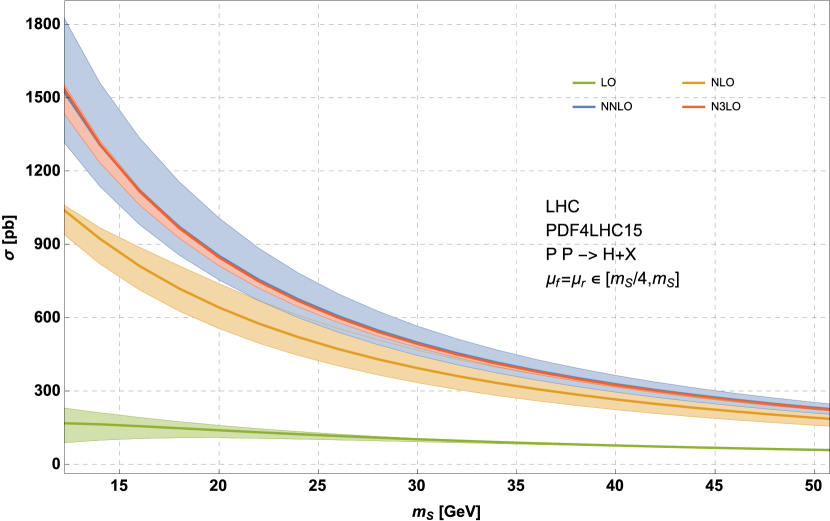
Figure 1: Effective theory production cross section of a scalar particle as a function of the particle mass mS[10,50]subscript𝑚𝑆1050m_{S}\in\left[10,50\right] GeV through increasing orders in perturbation theory, at a 13 TeV proton-proton collider. The bands enveloping the respective orders represent the variation of the cross section due to variations of the scale μ[mS/4,mS]𝜇subscript𝑚𝑆4subscript𝑚𝑆\mu\in\left[{m_{S}}/{4},m_{S}\right]. The value of the top mass is set to mt(mt)=162.7subscript𝑚𝑡subscript𝑚𝑡162.7m_{t}(m_{t})=162.7 GeV.
Refer to caption
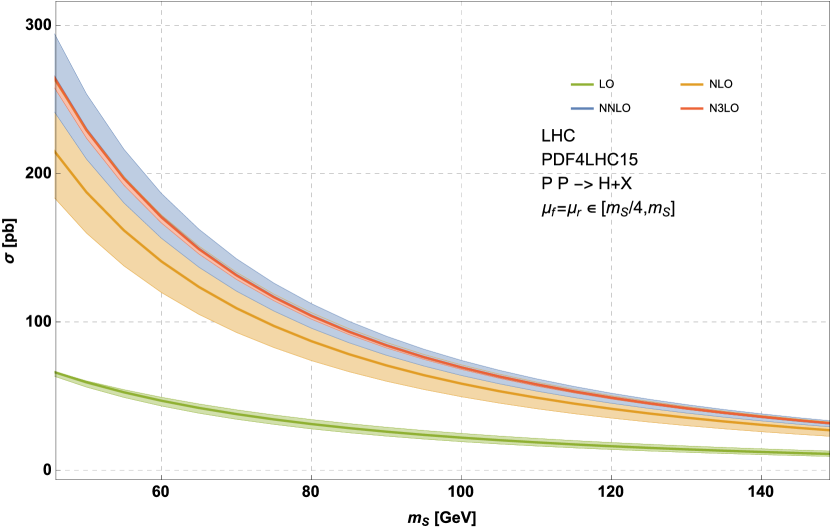
Figure 2: Effective theory production cross section of a scalar particle of mass mS[50,150]subscript𝑚𝑆50150m_{S}\in\left[50,150\right] GeV through increasing orders in perturbation theory. For further details see the caption of Fig. 1.
Refer to caption
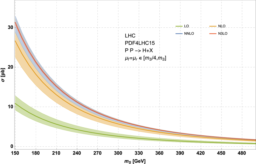
Figure 3: Effective theory production cross section of a scalar particle with mass mS[150,500]subscript𝑚𝑆150500m_{S}\in\left[150,500\right] GeV through increasing orders in perturbation theory. For further details see the caption of Fig. 1.
Refer to caption
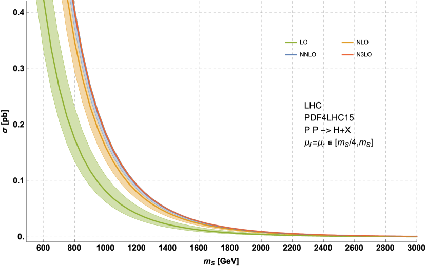
Figure 4: Effective theory production cross section of a scalar particle as a function of the particle mass mS[500,3000]subscript𝑚𝑆5003000m_{S}\in\left[500,3000\right] GeV through increasing orders in perturbation theory. For further details see the caption of Fig. 1.

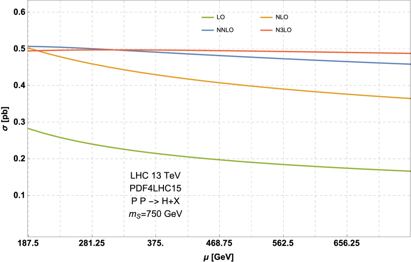
Let us now discuss our predictions for the production cross section σSsubscript𝜎𝑆\sigma_{S}. In Figs. 1 - 4 we show the effective theory cross section σH(mS,ΓS=0,mt)\sigma_{H}(m_{S},\Gamma_{S}=0,m_{t}) as a function of mSsubscript𝑚𝑆m_{S} through N3LO, at a proton-proton collider with a center-of-mass energy of 13 TeV. The theory uncertainty bands correspond to a variation of the scale μ=μr=μf𝜇subscript𝜇𝑟subscript𝜇𝑓\mu=\mu_{r}=\mu_{f} in the range μ[mS/4,mS]𝜇subscript𝑚𝑆4subscript𝑚𝑆\mu\in\left[{m_{S}}/{4},m_{S}\right]. The value of the top mass is set to mt(mt)=162.7subscript𝑚𝑡subscript𝑚𝑡162.7m_{t}(m_{t})=162.7 GeV and we use the PDF4LHC15 [27] parton distribution function (PDF) set. We observe that for the range of scalar masses between 10 GeV and 3 TeV the N3LO scale variation band is always contained inside the NNLO band. This is also true for the lowest values of this mass range, mS1050 GeVsimilar-tosubscript𝑚𝑆1050 GeVm_{S}\sim 10-50\textrm{ GeV} (Fig. 1), where one observes especially large corrections at NLO and NNLO. For higher masses, the scale variation is reduced. As an illustration, we show in Fig. 5 the scale dependence for the cross section of a CP-even scalar with a mass of 750 GeV.
Refer to caption
Figure 5: Effective theory production cross section of a scalar particle with a mass mS=subscript𝑚𝑆absentm_{S}= 750 GeV as a function of the common renormalization and factorization scales μ𝜇\mu through increasing orders in perturbation theory.

Sources of theoretical uncertainty affecting the gluon-fusion cross section at N3LO other than scale variation have been considered in detail in ref. [19]. In particular, these sources of uncertainty are due to the lack of N3LO parton densities and to the truncation of the threshold expansion for the N3LO correction. In order to estimate the uncertainty on our computation, we follow faithfully the uncertainty estimation prescription of ref. [19] with one modification: the uncertainty due to the lack of N3LO parton densities is estimated here as the envelope of the corresponding uncertainties formed by using the CT14 [28], NNPDF30 [29] and PDF4LHC sets, which are themselves computed according to the prescription of ref. [19]. The reason for modifying the prescription in this case is that the PDF4LHC set leads to very small uncertainties for scalars in the region 50010005001000500-1000 GeV and, in particular, to a vanishing uncertainty estimate for a scalar with mass around 770 GeV. This feature is not shared with individual PDF sets. We therefore use, conservatively, the envelope of CT14, NNPDF30 and PDF4LHC, which leads to an uncertainty due to the lack of N3LO parton densities at the level of 0.9%3%percent0.9percent30.9\%-3\% for scalars in the range 505050 GeV33-3 TeV. This uncertainty remains of the order of a few percent also at lower masses, but it increases rapidly to 𝒪(10%)𝒪percent10{\cal O}(10\%) for mS20less-than-or-similar-tosubscript𝑚𝑆20m_{S}\lesssim 20 GeV.

We present the cross section values and uncertainties for this range of scalar masses in Appendix A. In particular, in Tab. 6 we focus on the range between 730 and 770 GeV.

3 Finite width effects and the line-shape

The results of the previous section hold formally only when the width of the scalar is set to zero. In many beyond the Standard Model (BSM) scenarios, however, finite-width effects cannot be neglected. In this section we present a way to include leading finite-width effects into our results, in the case where the width is not too large compared to the mass.
The total cross section for the production of a scalar boson of total width ΓSsubscriptΓ𝑆\Gamma_{S} can be obtained from the cross section in the zero-width approximation via a convolution

σS(mS,ΓS,ΛUV)=𝑑Q2QΓS(Q)πσS(Q,ΓS=0,ΛUV)(Q2mS2)2+mS2Γ2(mS)+𝒪(ΓS(mS)/mS),\sigma_{S}(m_{S},\Gamma_{S},\Lambda_{\rm UV})=\int dQ^{2}\frac{Q\Gamma_{S}(Q)}{\pi}\frac{\sigma_{S}(Q,\Gamma_{S}=0,\Lambda_{\rm UV})}{(Q^{2}-m_{S}^{2})^{2}+m_{S}^{2}\Gamma^{2}(m_{S})}+\mathcal{O}\left(\Gamma_{S}(m_{S})/m_{S}\right)\,, (8)

where Q𝑄Q is the virtuality of the scalar particle. This expression is accurate at leading order in ΓS(mS)/mSsubscriptΓ𝑆subscript𝑚𝑆subscript𝑚𝑆\Gamma_{S}(m_{S})/m_{S}. For large values of the width relative to the mass, subleading corrections and signal-background interference effects are important and are not captured by eq. (8). Let us also note that in order to use eq. (8) faithfully, one needs the width as a function of the virtuality of the scalar, which may bear a substantial model dependence. However, it is often the case that the width can be approximated as

ΓS(QmS)ΓS.subscriptΓ𝑆𝑄subscript𝑚𝑆subscriptΓ𝑆\Gamma_{S}(Q\approx m_{S})\equiv\Gamma_{S}\,. (9)

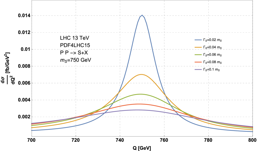
The invariant mass distribution in this approximation for the production of a CP-even scalar with a mass of mS=750subscript𝑚𝑆750m_{S}=750 GeV and total width from 2 to 10%percent1010\% of the scalar mass is shown in Fig. 6. This result has been obtained from an interpolation of the zero-width cross section values of Tab. 6 in Appendix A. We caution that if the results of Appendix A are used to derive cross section values with non-zero width effects following the strategy outlined in this section, an additional uncertainty of the order 𝒪(ΓS/mS)𝒪subscriptΓ𝑆subscript𝑚𝑆{\cal O}\left({\Gamma_{S}}/{m_{S}}\right) should be assigned.

Refer to caption
Figure 6: Line-shape of a 750 GeV CP-even scalar boson at the LHC for different values of its total width.

In order to facilitate the computation of the line-shape we perform a parametric fit of the production cross section of a zero-width scalar boson as a function of its virtuality (with ΛUV=mSsubscriptΛUVsubscript𝑚𝑆\Lambda_{\textrm{UV}}=m_{S}) for a center-of-mass energy of 131313TeV. To guarantee agreement of the fitted cross section with the actual cross section at a level better than 1%percent11\%, we split the range of interesting scalar boson mass values into three intervals:

  • in the range mS[10 GeV,150 GeV]subscript𝑚𝑆10 GeV150 GeVm_{S}\in[10\textrm{ GeV},150\textrm{ GeV}], cf. Tab. 2 in Appendix A, we find

    σS(x)subscript𝜎𝑆𝑥\displaystyle\sigma_{S}(x) \displaystyle\approx (3.89881×106x21.90274×106x202261xlog2x+1623.77log2x\displaystyle\left(3.89881\times 10^{6}\,x^{2}-1.90274\times 10^{6}\,x-202261\,x\,\log^{2}x+1623.77\,\log^{2}x\right. (10)
    \displaystyle- 923052xlogx+24108.2logx+95652.2) pb,\displaystyle\left.923052\,x\,\log x+24108.2\,\log x+95652.2\right)\textrm{ pb}\,,
  • in the range mS[150 GeV,500 GeV]subscript𝑚𝑆150 GeV500 GeVm_{S}\in[150\textrm{ GeV},500\textrm{ GeV}], cf. Tab. 3, we find

    σS(x)(1x3)9.52798x0.0415044logx1.50381 pb,subscript𝜎𝑆𝑥superscript13𝑥9.52798superscript𝑥0.0415044𝑥1.50381 pb\sigma_{S}(x)\approx\left(1-\sqrt[3]{x}\right)^{9.52798}\,x^{-0.0415044\,\log x-1.50381}\,\,\textrm{ pb}\,, (11)
  • in the range mS[500 GeV,3000 GeV]subscript𝑚𝑆500 GeV3000 GeVm_{S}\in[500\textrm{ GeV},3000\textrm{ GeV}], cf. Tabs. 4-5, we find

    σS(x)(1x3)9.71562x0.0040194log3x0.0474683log2x0.240878logx1.81243 pb,subscript𝜎𝑆𝑥superscript13𝑥9.71562superscript𝑥0.0040194superscript3𝑥0.0474683superscript2𝑥0.240878𝑥1.81243 pb\sigma_{S}(x)\approx\left(1-\sqrt[3]{x}\right)^{9.71562}\,x^{-0.0040194\,\log^{3}x-0.0474683\,\log^{2}x-0.240878\,\log x-1.81243}\textrm{ pb}\,, (12)

where xQ/GeV13 TeV𝑥𝑄GeV13 TeVx\equiv\frac{Q/\textrm{GeV}}{13\textrm{ TeV}}. The fits of Eqs. (10)-(12) can be used as the kernel of the convolution in eq. (8).

4 Validity of the EFT approach

So far, we have assumed that the effective theory of eq. (1) furnishes an accurate description of the gluon-scalar interaction. However, this assumption may be challenged if the scalar couples to light coloured particles. To investigate this effect, we will consider a scalar of mass mS=750subscript𝑚𝑆750m_{S}=750 GeV which couples to a top-like quark of mass mTsubscript𝑚𝑇m_{T}. In this scenario, we can compute the cross-section exactly through NLO in perturbative QCD. We can then compare this prediction with the cross-section derived with the effective theory of eq. (1).

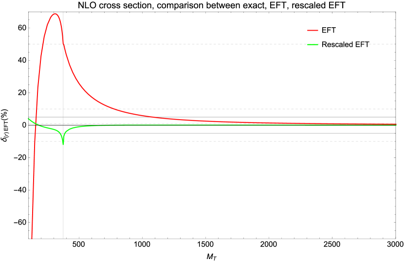
The red line in Fig. 7 shows the percent difference of the two predictions,

δEFT=σexactNLOσEFTNLOσexactNLO×100%,subscript𝛿EFTsubscriptsuperscript𝜎NLOexactsubscriptsuperscript𝜎NLOEFTsubscriptsuperscript𝜎NLOexactpercent100\delta_{\rm EFT}=\frac{\sigma^{\rm NLO}_{\rm exact}-\sigma^{\rm NLO}_{\rm EFT}}{\sigma^{\rm NLO}_{\rm exact}}\times 100\%\;, (13)

as a function of mTsubscript𝑚𝑇m_{T} for a scalar with a mass of mS=750subscript𝑚𝑆750m_{S}=750 GeV. While in the region mTmS/2similar-tosubscript𝑚𝑇subscript𝑚𝑆2m_{T}\sim m_{S}/2 the effective field theory is inadequate, for larger values of mTsubscript𝑚𝑇m_{T} the EFT description becomes accurate very quickly. Indeed, for mT1.5mSsimilar-tosubscript𝑚𝑇1.5subscript𝑚𝑆m_{T}\sim 1.5m_{S} the discrepancy with respect to the exact result is already below the theoretical uncertainty of QCD origin (of about 5%percent55\%).

Refer to caption
Figure 7: Percent difference (15) between the exact and rescaled EFT (rEFT) cross section at NLO (red line/green line) as a function of the quark mass for the production of a 750 GeV CP-even scalar. The vertical line corresponds to mS/2subscript𝑚𝑆2m_{S}/2.

Let us now define a rescaled effective theory cross-section,

σrEFTNLO=σexactLOσEFTLOσEFTNLO.subscriptsuperscript𝜎NLOrEFTsubscriptsuperscript𝜎LOexactsubscriptsuperscript𝜎LOEFTsubscriptsuperscript𝜎NLOEFT\sigma^{\rm NLO}_{\rm rEFT}=\frac{\sigma^{{\rm LO}}_{\rm exact}}{\sigma^{{\rm LO}}_{\rm EFT}}\,\sigma^{{\rm NLO}}_{\rm EFT}\;. (14)

The green line of Fig. 7 shows the relative difference

δrEFT=100×σexactNLOσrEFTNLOσexactNLOsubscript𝛿rEFT100subscriptsuperscript𝜎NLOexactsubscriptsuperscript𝜎NLOrEFTsubscriptsuperscript𝜎NLOexact\delta_{\rm rEFT}=100\times\,\frac{\sigma^{\rm NLO}_{\rm exact}-\sigma^{\rm NLO}_{\rm rEFT}}{\sigma^{\rm NLO}_{\rm exact}} (15)

between the rescaled effective theory prediction for the cross-section and the exact NLO cross section. We notice that the rescaled effective theory cross-section reproduces the exact cross section very well (as it has also been the case for the Standard Model Higgs boson [30, 31]).

We conclude that, while for the study of scalars which couple to relatively light particles one should resort to a calculation within a specific model, also in such situations the effective theory computation can be utilised as a means to compute with a good accuracy the corresponding QCD Klimit-from𝐾K- factor with respect to the exact LO cross section.

5 Top-quark contributions

So far we have considered the case where the interaction between the heavy scalar S𝑆S and the Standard Model is mediated exclusively by the dimension-five operator in eq. (1). In many extensions of the Standard Model new scalars may also couple directly to the quarks of the third generation as well as the W𝑊W and Z𝑍Z bosons. However, the absence of resonances in top-pair production and four-lepton production suggests that these couplings should be small. It may be nonetheless useful to estimate the contribution to the inclusive S𝑆S-scalar cross section due to the heavy SM quarks and gauge bosons for the purpose of setting precise experimental constraints on their couplings to S𝑆S. In this section, we study the effects due to the top quark, which in many scenarios are expected to give the most important contribution.

For light scalar masses, mS<𝒪(mt)subscript𝑚𝑆𝒪subscript𝑚𝑡m_{S}<{\cal O}(m_{t}), contributions due to the coupling of the top quark can be simply taken into account through N3LO in perturbative QCD by using an appropriate Wilson coefficient CSsubscript𝐶𝑆C_{S}. For heavier scalars with masses around and above the top-pair threshold, however, it is not justified theoretically to integrate out the top-quark. For this reason we study in the following the effect of modifying the Largangian in eq. (1) by including a direct Yukawa interaction between the scalar S𝑆S and the top quark, i.e., we consider the Lagrangian

eff=SM+Sλwc4vCSGμνaGaμνλtmtvSt¯t,subscripteffsubscriptSMsubscript𝑆subscript𝜆wc4𝑣𝐶𝑆superscriptsubscript𝐺𝜇𝜈𝑎superscriptsubscript𝐺𝑎𝜇𝜈subscript𝜆𝑡subscript𝑚𝑡𝑣𝑆¯𝑡𝑡\mathcal{L}_{\text{eff}}=\mathcal{L}_{\textrm{SM}}+\mathcal{L}_{S}-\frac{\lambda_{\rm wc}}{4v}C\,S\,G_{\mu\nu}^{a}G_{a}^{\mu\nu}-\lambda_{t}\frac{m_{t}}{v}\,S\,\bar{t}t\,, (16)

where λtsubscript𝜆𝑡\lambda_{t} is the ratio of the Yukawa coupling of the scalar S𝑆S and the Yukawa coupling of the Higgs boson to the top quark and λwc=CSCsubscript𝜆wcsubscript𝐶𝑆𝐶\lambda_{\rm wc}=\frac{C_{S}}{C} denotes the ratio of the Wilson coefficients in this theory and the SM with the top-quark integrated out.
Refer to caption
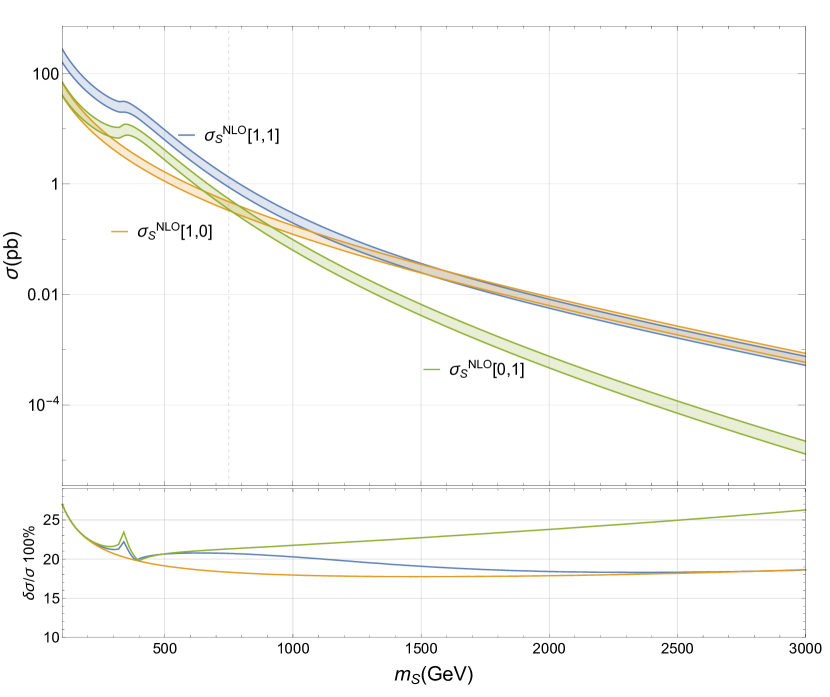
Figure 8: NLO contributions to the total cross section for a scalar particle of mass mSsubscript𝑚𝑆m_{S} as described in eqs. (18), (19). The bands correspond to the theory uncertainty (based on eq. (20)). In the lower pane we present the relative theory uncertainty (%percent\%) for each of the contributions.

The production cross section now depends on the values of λwcsubscript𝜆wc\lambda_{\rm wc} and λtsubscript𝜆𝑡\lambda_{t}:

σSσS[λwc,λt].subscript𝜎𝑆subscript𝜎𝑆subscript𝜆wcsubscript𝜆𝑡\sigma_{S}\equiv\sigma_{S}[\lambda_{\rm wc},\lambda_{t}]\,. (17)

It does not take too much effort to show that the NLO cross section can be cast in the form

σSNLO[λwc,λt]=λwc(λwcλt)σSNLO[1,0]+λt(λtλwc)σSNLO[0,1]+λwcλtσSNLO[1,1].superscriptsubscript𝜎𝑆NLOsubscript𝜆wcsubscript𝜆𝑡subscript𝜆wcsubscript𝜆wcsubscript𝜆𝑡superscriptsubscript𝜎𝑆NLO10subscript𝜆𝑡subscript𝜆𝑡subscript𝜆wcsuperscriptsubscript𝜎𝑆NLO01subscript𝜆wcsubscript𝜆𝑡superscriptsubscript𝜎𝑆NLO11\begin{split}\sigma_{S}^{\rm NLO}[\lambda_{\rm wc},\lambda_{t}]&\,=\lambda_{\rm wc}(\lambda_{\rm wc}-\lambda_{t})\sigma_{S}^{\rm NLO}[1,0]+\lambda_{t}(\lambda_{t}-\lambda_{\rm wc})\sigma_{S}^{\rm NLO}[0,1]\\ &\,+\lambda_{\rm wc}\lambda_{t}\,\sigma_{S}^{\rm NLO}[1,1]\,.\end{split} (18)

The cross section with no Yukawa coupling, σSNLO[1,0]superscriptsubscript𝜎𝑆NLO10\sigma_{S}^{\rm NLO}[1,0], is known through N3LO. Hence, we can improve the previous expression by including all N3LO corrections to the terms proportional to λwc2superscriptsubscript𝜆wc2\lambda_{\rm wc}^{2},

σS[λwc,λt]=λwc2σSN3LO[1,0]λwcλtσSNLO[1,0]+λt(λtλwc)σSNLO[0,1]+λwcλtσSNLO[1,1].subscript𝜎𝑆subscript𝜆wcsubscript𝜆𝑡superscriptsubscript𝜆wc2superscriptsubscript𝜎𝑆superscriptN3LO10subscript𝜆wcsubscript𝜆𝑡superscriptsubscript𝜎𝑆NLO10subscript𝜆𝑡subscript𝜆𝑡subscript𝜆wcsuperscriptsubscript𝜎𝑆NLO01subscript𝜆wcsubscript𝜆𝑡superscriptsubscript𝜎𝑆NLO11\begin{split}\sigma_{S}[\lambda_{\rm wc},\lambda_{t}]&\,=\lambda_{\rm wc}^{2}\sigma_{S}^{\textrm{N}^{3}\textrm{LO}}[1,0]-\lambda_{\rm wc}\lambda_{t}\sigma_{S}^{\rm NLO}[1,0]+\lambda_{t}(\lambda_{t}-\lambda_{\rm wc})\sigma_{S}^{\rm NLO}[0,1]\\ &\,+\lambda_{\rm wc}\lambda_{t}\,\sigma_{S}^{\rm NLO}[1,1]\,.\end{split} (19)
s𝑠\sqrt{s} Component value[fb] δ𝛿\delta(theory) [%percent\%] δ𝛿\delta(pdf+αSsubscript𝛼𝑆\alpha_{S}) [%percent\%]
7 TeV σSN3LO[1,0]superscriptsubscript𝜎𝑆superscriptN3LO10\sigma_{S}^{\textrm{N}^{3}\textrm{LO}}[1,0] 69.72 4.2+2.0subscriptsuperscriptabsent2.04.2{}^{+2.0}_{-4.2} 7.0
σSNLO[1,0]superscriptsubscript𝜎𝑆NLO10\sigma_{S}^{\rm NLO}[1,0] 55.59 19.52 6.95
σSNLO[0,1]superscriptsubscript𝜎𝑆NLO01\sigma_{S}^{\rm NLO}[0,1] 61.71 22.69 6.94
σSNLO[1,1]superscriptsubscript𝜎𝑆NLO11\sigma_{S}^{\rm NLO}[1,1] 152.6 22.1 6.92
8 TeV σSN3LO[1,0]superscriptsubscript𝜎𝑆superscriptN3LO10\sigma_{S}^{\textrm{N}^{3}\textrm{LO}}[1,0] 111.4 4.0+1.9subscriptsuperscriptabsent1.94.0{}^{+1.9}_{-4.0} 6.1
σSNLO[1,0]superscriptsubscript𝜎𝑆NLO10\sigma_{S}^{\rm NLO}[1,0] 89.37 19.18 6.23
σSNLO[0,1]superscriptsubscript𝜎𝑆NLO01\sigma_{S}^{\rm NLO}[0,1] 98.92 22.3 6.22
σSNLO[1,1]superscriptsubscript𝜎𝑆NLO11\sigma_{S}^{\rm NLO}[1,1] 245.3 21.71 6.2
13 TeV σSN3LO[1,0]superscriptsubscript𝜎𝑆superscriptN3LO10\sigma_{S}^{\textrm{N}^{3}\textrm{LO}}[1,0] 496.9 3.7+2.0subscriptsuperscriptabsent2.03.7{}^{+2.0}_{-3.7} 4.0
σSNLO[1,0]superscriptsubscript𝜎𝑆NLO10\sigma_{S}^{\rm NLO}[1,0] 404.6 18.3 4.5
σSNLO[0,1]superscriptsubscript𝜎𝑆NLO01\sigma_{S}^{\rm NLO}[0,1] 442.7 21.3 4.4
σSNLO[1,1]superscriptsubscript𝜎𝑆NLO11\sigma_{S}^{\rm NLO}[1,1] 1108 20.7 4.4
14 TeV σSN3LO[1,0]superscriptsubscript𝜎𝑆superscriptN3LO10\sigma_{S}^{\textrm{N}^{3}\textrm{LO}}[1,0] 609.7 3.7+1.9subscriptsuperscriptabsent1.93.7{}^{+1.9}_{-3.7} 3.8
σSNLO[1,0]superscriptsubscript𝜎𝑆NLO10\sigma_{S}^{\rm NLO}[1,0] 497.3 18.21 4.26
σSNLO[0,1]superscriptsubscript𝜎𝑆NLO01\sigma_{S}^{\rm NLO}[0,1] 543. 21.14 4.2
σSNLO[1,1]superscriptsubscript𝜎𝑆NLO11\sigma_{S}^{\rm NLO}[1,1] 1361 20.57 4.21
Table 1: Contributions to the cross section (19) for the production of a CP-even scalar with mass 750 GeV at a proton-proton collider.

Although we have taken into account QCD corrections within the EFT framework through N3LO , the result for the cross section is formally only NLO-accurate because we are missing finite-mass effects beyond NLO. We therefore estimate the uncertainties on the NLO cross-section as

δσNLO[n1,n2]σNLO[n1,n2]=±δ>NLO(1+δscheme[n1,n2]),ni{0,1},formulae-sequence𝛿superscript𝜎NLOsubscript𝑛1subscript𝑛2superscript𝜎NLOsubscript𝑛1subscript𝑛2plus-or-minussubscript𝛿absentNLO1subscript𝛿schemesubscript𝑛1subscript𝑛2subscript𝑛𝑖01\frac{\delta\sigma^{\rm NLO}[n_{1},n_{2}]}{\sigma^{\rm NLO}[n_{1},n_{2}]}=\pm\delta_{>{\rm NLO}}\,(1+\delta_{\rm scheme}[n_{1},n_{2}])\,,\quad n_{i}\in\{0,1\}\,, (20)

where

δ>NLO=(σN3LO[1,0]σNLO[1,0]σNLO[1,0])EFTsubscript𝛿absentNLOsubscriptsuperscript𝜎superscriptN3LO10superscript𝜎NLO10superscript𝜎NLO10EFT\delta_{>{\rm NLO}}=\left(\frac{\sigma^{\rm N^{3}LO}[1,0]-\sigma^{\rm NLO}[1,0]}{\sigma^{\rm NLO}[1,0]}\right)_{\rm EFT} (21)

is the relative change of the gluon-fusion cross-section in the effective theory from NLO to N3LO. Note that in this way make the assumption that the cross-section components that are not known beyond NLO will not have a worse perturbative convergence than in the effective theory. Finally, we enlarge this uncertainty further by

δscheme[n1,n2]=|σexactNLO,MS¯[n1,n2]σexactNLO,OS[n1,n2]|σexactNLO,MS¯[n1,n2],subscript𝛿schemesubscript𝑛1subscript𝑛2subscriptsuperscript𝜎NLO¯MSexactsubscript𝑛1subscript𝑛2subscriptsuperscript𝜎NLOOSexactsubscript𝑛1subscript𝑛2subscriptsuperscript𝜎NLO¯MSexactsubscript𝑛1subscript𝑛2\delta_{\rm scheme}[n_{1},n_{2}]=\frac{\left|\sigma^{\rm NLO,\overline{MS}}_{\textrm{exact}}[n_{1},n_{2}]-\sigma^{\rm NLO,OS}_{\textrm{exact}}[n_{1},n_{2}]\right|}{\sigma^{\rm NLO,\overline{MS}}_{\textrm{exact}}[n_{1},n_{2}]}\;, (22)

which measures the scheme dependence of the top-quark contribution at NLO.

Equation (19) is our best prediction for the gluon-fusion production cross section of a generic scalar S𝑆S. We recall that the values of σSN3LO[1,0]superscriptsubscript𝜎𝑆superscriptN3LO10\sigma_{S}^{\textrm{N}^{3}\textrm{LO}}[1,0] as a function of the scalar boson mass can be read off from Tabs. 2-5 in Appendix A. The NLO cross sections σSNLO[n1,n2]superscriptsubscript𝜎𝑆NLOsubscript𝑛1subscript𝑛2\sigma_{S}^{\rm NLO}[n_{1},n_{2}] (n1,n2{0,1}subscript𝑛1subscript𝑛201n_{1},n_{2}\in\{0,1\}) are reported in Tabs. 7-14. As an illustration, we present the complete set of terms entering in eq. (19) for a scalar of mass mS=750 GeVsubscript𝑚𝑆750 GeVm_{S}=750\textrm{ GeV} in Tab. 1.

The following fits are a good approximation to the central values of the cross sections introduced in this section. The fits are functions of x=mS/GeV13TeV𝑥subscript𝑚𝑆GeV13TeVx=\frac{m_{S}/\textrm{GeV}}{13\textrm{TeV}} valid for a center-of-mass energy of 131313TeV and PDF4LHC15 parton distribution functions.

  • In the range mS[50 GeV,150 GeV]subscript𝑚𝑆50 GeV150 GeVm_{S}\in[50\textrm{ GeV},150\textrm{ GeV}], we find

    σSNLO[1,1]/pb=4.79097×109x2454.08x248.2912logxx2+1.4105×109x1.22684×106x+1.79376×107log2x+1.11478×109xlogx+1.59613×108logx168047logxx+4.39955×108,superscriptsubscript𝜎𝑆NLO11pbabsent4.79097superscript109superscript𝑥2454.08superscript𝑥248.2912𝑥superscript𝑥21.4105superscript109𝑥missing-subexpression1.22684superscript106𝑥1.79376superscript107superscript2𝑥1.11478superscript109𝑥𝑥missing-subexpression1.59613superscript108𝑥168047𝑥𝑥4.39955superscript108\displaystyle\begin{aligned} \sigma_{S}^{\textrm{NLO}}[1,1]/\textrm{pb}&=-4.79097\times 10^{9}x^{2}-\frac{454.08}{x^{2}}-\frac{48.2912\log x}{x^{2}}+1.4105\times 10^{9}x\\ &-\frac{1.22684\times 10^{6}}{x}+1.79376\times 10^{7}\log^{2}x+1.11478\times 10^{9}x\log x\\ &+1.59613\times 10^{8}\log x-\frac{168047\log x}{x}+4.39955\times 10^{8}\,,\end{aligned} (23)
    σSNLO[1,0]/pb=2.71176×109x2+302.023x2+32.2322logxx28.07812×108x+787193x1.11305×107log2x6.62451×108xlogx9.8134×107logx+108365logxx2.68924×108,superscriptsubscript𝜎𝑆NLO10pbabsent2.71176superscript109superscript𝑥2302.023superscript𝑥232.2322𝑥superscript𝑥28.07812superscript108𝑥missing-subexpression787193𝑥1.11305superscript107superscript2𝑥6.62451superscript108𝑥𝑥missing-subexpression9.8134superscript107𝑥108365𝑥𝑥2.68924superscript108\displaystyle\begin{aligned} \sigma_{S}^{\textrm{NLO}}[1,0]/\textrm{pb}&=2.71176\times 10^{9}x^{2}+\frac{302.023}{x^{2}}+\frac{32.2322\log x}{x^{2}}-8.07812\times 10^{8}x\\ &+\frac{787193}{x}-1.11305\times 10^{7}\log^{2}x-6.62451\times 10^{8}x\log x\\ &-9.8134\times 10^{7}\log x+\frac{108365\log x}{x}-2.68924\times 10^{8}\,,\end{aligned}
    σSNLO[0,1]/pb=9109703.05552×107x2+7.62007×106x544.886x+26407.1log2x+3.86595×106xlogx+290640logx58.3182logxx.superscriptsubscript𝜎𝑆NLO01pbabsent9109703.05552superscript107superscript𝑥27.62007superscript106𝑥544.886𝑥missing-subexpression26407.1superscript2𝑥3.86595superscript106𝑥𝑥290640𝑥missing-subexpression58.3182𝑥𝑥\displaystyle\begin{aligned} \sigma_{S}^{\textrm{NLO}}[0,1]/\textrm{pb}&=910970-3.05552\times 10^{7}x^{2}+7.62007\times 10^{6}x-\frac{544.886}{x}\\ &+26407.1\log^{2}x+3.86595\times 10^{6}x\log x+290640\log x\\ &-\frac{58.3182\log x}{x}\,.\end{aligned} (24)
  • In the range mS[150 GeV,350 GeV]subscript𝑚𝑆150 GeV350 GeVm_{S}\in[150\textrm{ GeV},350\textrm{ GeV}], we find

    σSNLO[1,1]/pb=5.78391×1011x36.04905×1012x3logx3.97065×1012x21.60239×1012x2logx2.28312×1011x7.35167×106x+1.05353×108log2x4.9669×1010xlogx+6.11874×108logx865250logxx+5.46682×108,superscriptsubscript𝜎𝑆NLO11pbabsent5.78391superscript1011superscript𝑥36.04905superscript1012superscript𝑥3𝑥3.97065superscript1012superscript𝑥2missing-subexpression1.60239superscript1012superscript𝑥2𝑥2.28312superscript1011𝑥7.35167superscript106𝑥missing-subexpression1.05353superscript108superscript2𝑥4.9669superscript1010𝑥𝑥missing-subexpression6.11874superscript108𝑥865250𝑥𝑥5.46682superscript108\displaystyle\begin{aligned} \sigma_{S}^{\textrm{NLO}}[1,1]/\textrm{pb}&=5.78391\times 10^{11}x^{3}-6.04905\times 10^{12}x^{3}\log x-3.97065\times 10^{12}x^{2}\\ &-1.60239\times 10^{12}x^{2}\log x-2.28312\times 10^{11}x-\frac{7.35167\times 10^{6}}{x}\\ &+1.05353\times 10^{8}\log^{2}x-4.9669\times 10^{10}x\log x\\ &+6.11874\times 10^{8}\log x-\frac{865250\log x}{x}+5.46682\times 10^{8}\,,\end{aligned}
    σSNLO[1,0]/pb=1.18403×1010x3+8.55496×1010x3logx+5.7597×1010x2+2.3659×1010x2logx+3.48892×109x+121488.x1.66608×106log2x+7.67582×108xlogx9.42982×106logx+14369.3logxx7.62306×106,\displaystyle\begin{aligned} \sigma_{S}^{\textrm{NLO}}[1,0]/\textrm{pb}&=-1.18403\times 10^{10}x^{3}+8.55496\times 10^{10}x^{3}\log x+5.7597\times 10^{10}x^{2}\\ &+2.3659\times 10^{10}x^{2}\log x+3.48892\times 10^{9}x+\frac{121488.}{x}\\ &-1.66608\times 10^{6}\log^{2}x+7.67582\times 10^{8}x\log x\\ &-9.42982\times 10^{6}\log x+\frac{14369.3\log x}{x}-7.62306\times 10^{6}\,,\end{aligned}
    σSNLO[0,1]/pb=3.58507×1011x33.67114×1012x3logx2.41271×1012x29.74512×1011x2logx1.3909×1011x4.49756×106x+6.4297×107log2x3.02763×1010xlogx+3.72922×108logx529486logxx+3.31551×108.superscriptsubscript𝜎𝑆NLO01pbabsent3.58507superscript1011superscript𝑥33.67114superscript1012superscript𝑥3𝑥2.41271superscript1012superscript𝑥2missing-subexpression9.74512superscript1011superscript𝑥2𝑥1.3909superscript1011𝑥4.49756superscript106𝑥missing-subexpression6.4297superscript107superscript2𝑥3.02763superscript1010𝑥𝑥missing-subexpression3.72922superscript108𝑥529486𝑥𝑥3.31551superscript108\displaystyle\begin{aligned} \sigma_{S}^{\textrm{NLO}}[0,1]/\textrm{pb}&=3.58507\times 10^{11}x^{3}-3.67114\times 10^{12}x^{3}\log x-2.41271\times 10^{12}x^{2}\\ &-9.74512\times 10^{11}x^{2}\log x-1.3909\times 10^{11}x-\frac{4.49756\times 10^{6}}{x}\\ &+6.4297\times 10^{7}\log^{2}x-3.02763\times 10^{10}x\log x\\ &+3.72922\times 10^{8}\log x-\frac{529486\log x}{x}+3.31551\times 10^{8}\,.\end{aligned}
  • In the range mS[350 GeV,500 GeV]subscript𝑚𝑆350 GeV500 GeVm_{S}\in[350\textrm{ GeV},500\textrm{ GeV}], we find

    σSNLO[1,1]/pb=1.55048×1010x2+20602.3x2+4.12759×1010x2logx+3.27683×1010x+3.90175×106x1.00487×108log2x1.21312×106log2xx+1.28157×1010xlogx1.37351×108logx6.26022×106logxx+8.75837×108,superscriptsubscript𝜎𝑆NLO11pbabsent1.55048superscript1010superscript𝑥220602.3superscript𝑥24.12759superscript1010superscript𝑥2𝑥missing-subexpression3.27683superscript1010𝑥3.90175superscript106𝑥1.00487superscript108superscript2𝑥missing-subexpression1.21312superscript106superscript2𝑥𝑥1.28157superscript1010𝑥𝑥missing-subexpression1.37351superscript108𝑥6.26022superscript106𝑥𝑥8.75837superscript108\displaystyle\begin{aligned} \sigma_{S}^{\textrm{NLO}}[1,1]/\textrm{pb}&=-1.55048\times 10^{10}x^{2}+\frac{20602.3}{x^{2}}+4.12759\times 10^{10}x^{2}\log x\\ &+3.27683\times 10^{10}x+\frac{3.90175\times 10^{6}}{x}-1.00487\times 10^{8}\log^{2}x\\ &-\frac{1.21312\times 10^{6}\log^{2}x}{x}+1.28157\times 10^{10}x\log x\\ &-1.37351\times 10^{8}\log x-\frac{6.26022\times 10^{6}\log x}{x}+8.75837\times 10^{8}\,,\end{aligned}
    σSNLO[1,0]/pb=1.74667×109x2+2345.03x2+4.57918×109x2logx+3.64833×109x+450670x1.12934×107log2x137023log2xx+1.43013×109xlogx1.53273×107logx704422logxx+9.83324×107,superscriptsubscript𝜎𝑆NLO10pbabsent1.74667superscript109superscript𝑥22345.03superscript𝑥24.57918superscript109superscript𝑥2𝑥missing-subexpression3.64833superscript109𝑥450670𝑥1.12934superscript107superscript2𝑥missing-subexpression137023superscript2𝑥𝑥1.43013superscript109𝑥𝑥1.53273superscript107𝑥missing-subexpression704422𝑥𝑥9.83324superscript107\displaystyle\begin{aligned} \sigma_{S}^{\textrm{NLO}}[1,0]/\textrm{pb}&=-1.74667\times 10^{9}x^{2}+\frac{2345.03}{x^{2}}+4.57918\times 10^{9}x^{2}\log x\\ &+3.64833\times 10^{9}x+\frac{450670}{x}-1.12934\times 10^{7}\log^{2}x\\ &-\frac{137023\log^{2}x}{x}+1.43013\times 10^{9}x\log x-1.53273\times 10^{7}\log x\\ &-\frac{704422\log x}{x}+9.83324\times 10^{7}\,,\end{aligned}
    σSNLO[0,1]/pb=1.59986×109x22171.87x24.2072×109x2logx3.34991×109x417719x+1.03789×107log2x+126226log2xx1.3131×109xlogx+1.40646×107logx+647893logxx9.03229×107.superscriptsubscript𝜎𝑆NLO01pbabsent1.59986superscript109superscript𝑥22171.87superscript𝑥24.2072superscript109superscript𝑥2𝑥missing-subexpression3.34991superscript109𝑥417719𝑥1.03789superscript107superscript2𝑥missing-subexpression126226superscript2𝑥𝑥1.3131superscript109𝑥𝑥1.40646superscript107𝑥missing-subexpression647893𝑥𝑥9.03229superscript107\displaystyle\begin{aligned} \sigma_{S}^{\textrm{NLO}}[0,1]/\textrm{pb}&=1.59986\times 10^{9}x^{2}-\frac{2171.87}{x^{2}}-4.2072\times 10^{9}x^{2}\log x\\ &-3.34991\times 10^{9}x-\frac{417719}{x}+1.03789\times 10^{7}\log^{2}x\\ &+\frac{126226\log^{2}x}{x}-1.3131\times 10^{9}x\log x+1.40646\times 10^{7}\log x\\ &+\frac{647893\log x}{x}-9.03229\times 10^{7}\,.\end{aligned}
  • In the range mS[500 GeV,1000 GeV]subscript𝑚𝑆500 GeV1000 GeVm_{S}\in[500\textrm{ GeV},1000\textrm{ GeV}], we find

    σSNLO[1,1]/pb=1.0459×108x2+478.474x27.72699×107x2logx8.14486×107x2.50557×106x95661.5log2x71863.4log2xx7.67177×107xlogx1.27372×107logx802665logxx3.08306×107,superscriptsubscript𝜎𝑆NLO11pbabsent1.0459superscript108superscript𝑥2478.474superscript𝑥27.72699superscript107superscript𝑥2𝑥missing-subexpression8.14486superscript107𝑥2.50557superscript106𝑥95661.5superscript2𝑥missing-subexpression71863.4superscript2𝑥𝑥7.67177superscript107𝑥𝑥missing-subexpression1.27372superscript107𝑥802665𝑥𝑥3.08306superscript107\displaystyle\begin{aligned} \sigma_{S}^{\textrm{NLO}}[1,1]/\textrm{pb}&=1.0459\times 10^{8}x^{2}+\frac{478.474}{x^{2}}-7.72699\times 10^{7}x^{2}\log x\\ &-8.14486\times 10^{7}x-\frac{2.50557\times 10^{6}}{x}-95661.5\log^{2}x\\ &-\frac{71863.4\log^{2}x}{x}-7.67177\times 10^{7}x\log x\\ &-1.27372\times 10^{7}\log x-\frac{802665\log x}{x}-3.08306\times 10^{7}\,,\end{aligned} (25)
    σSNLO[1,0]/pb=1.76181×107x2+81.1265x21.3039×107x2logx1.37328×107x421944x16421.7log2x12116.3log2xx1.29224×107xlogx2.14537×106logx135235logxx5.19164×106,superscriptsubscript𝜎𝑆NLO10pbabsent1.76181superscript107superscript𝑥281.1265superscript𝑥21.3039superscript107superscript𝑥2𝑥missing-subexpression1.37328superscript107𝑥421944𝑥16421.7superscript2𝑥missing-subexpression12116.3superscript2𝑥𝑥1.29224superscript107𝑥𝑥missing-subexpression2.14537superscript106𝑥135235𝑥𝑥5.19164superscript106\displaystyle\begin{aligned} \sigma_{S}^{\textrm{NLO}}[1,0]/\textrm{pb}&=1.76181\times 10^{7}x^{2}+\frac{81.1265}{x^{2}}-1.3039\times 10^{7}x^{2}\log x\\ &-1.37328\times 10^{7}x-\frac{421944}{x}-16421.7\log^{2}x\\ &-\frac{12116.3\log^{2}x}{x}-1.29224\times 10^{7}x\log x\\ &-2.14537\times 10^{6}\log x-\frac{135235\log x}{x}-5.19164\times 10^{6}\,,\end{aligned} (26)
    σSNLO[0,1]/pb=2.43245×107x2+110.92x21.78774×107x2logx1.88708×107x585093x22465.3log2x16766.8log2xx1.78573×107xlogx2.97483×106logx187382logxx7.19613×106.superscriptsubscript𝜎𝑆NLO01pbabsent2.43245superscript107superscript𝑥2110.92superscript𝑥21.78774superscript107superscript𝑥2𝑥missing-subexpression1.88708superscript107𝑥585093𝑥22465.3superscript2𝑥missing-subexpression16766.8superscript2𝑥𝑥1.78573superscript107𝑥𝑥missing-subexpression2.97483superscript106𝑥187382𝑥𝑥7.19613superscript106\displaystyle\begin{aligned} \sigma_{S}^{\textrm{NLO}}[0,1]/\textrm{pb}&=2.43245\times 10^{7}x^{2}+\frac{110.92}{x^{2}}-1.78774\times 10^{7}x^{2}\log x\\ &-1.88708\times 10^{7}x-\frac{585093}{x}-22465.3\log^{2}x\\ &-\frac{16766.8\log^{2}x}{x}-1.78573\times 10^{7}x\log x\\ &-2.97483\times 10^{6}\log x-\frac{187382\log x}{x}-7.19613\times 10^{6}\,.\end{aligned} (27)
  • In the range mS[1000 GeV,3000 GeV]subscript𝑚𝑆1000 GeV3000 GeVm_{S}\in[1000\textrm{ GeV},3000\textrm{ GeV}], we find

    σSNLO[1,1]/fb=x0.407849log3x0.841896log2x+77.9612xlogx+14.6265logx+49.7825×(1x3)1.74158,superscriptsubscript𝜎𝑆NLO11fbabsentsuperscript𝑥0.407849superscript3𝑥0.841896superscript2𝑥77.9612𝑥𝑥14.6265𝑥49.7825missing-subexpressionabsentsuperscript13𝑥1.74158\displaystyle\begin{aligned} \sigma_{S}^{\textrm{NLO}}[1,1]/\textrm{fb}&=x^{-0.407849\log^{3}x-0.841896\log^{2}x+77.9612x\log x+14.6265\log x+49.7825}\\ &\times\left(1-\sqrt[3]{x}\right)^{-1.74158}\,,\end{aligned} (28)
    σSNLO[1,0]/fb=x0.0682707log3x0.812125log2x2.68171xlogx3.91644logx10.0547×(1x3)7.95188,superscriptsubscript𝜎𝑆NLO10fbabsentsuperscript𝑥0.0682707superscript3𝑥0.812125superscript2𝑥2.68171𝑥𝑥3.91644𝑥10.0547missing-subexpressionabsentsuperscript13𝑥7.95188\displaystyle\begin{aligned} \sigma_{S}^{\textrm{NLO}}[1,0]/\textrm{fb}&=x^{-0.0682707\log^{3}x-0.812125\log^{2}x-2.68171x\log x-3.91644\log x-10.0547}\\ &\times\left(1-\sqrt[3]{x}\right)^{7.95188}\,,\end{aligned} (29)
    σSNLO[0,1]/fb=x2.40603x+0.812624log2x+18.7175xlogx+6.90869logx+12.7991×(1x3)8.05859.superscriptsubscript𝜎𝑆NLO01fbabsentsuperscript𝑥2.40603𝑥0.812624superscript2𝑥18.7175𝑥𝑥6.90869𝑥12.7991missing-subexpressionabsentsuperscript13𝑥8.05859\displaystyle\begin{aligned} \sigma_{S}^{\textrm{NLO}}[0,1]/\textrm{fb}&=x^{-2.40603x+0.812624\log^{2}x+18.7175x\log x+6.90869\log x+12.7991}\\ &\times\left(1-\sqrt[3]{x}\right)^{8.05859}\,.\end{aligned} (30)

6 Conclusion

In this paper we have presented the most precise predictions for the production of a CP-even scalar produced in gluon fusion at the LHC. We assume that the coupling of the scalar to the gluons can be described in an effective field theory approach. This enables us to provide precision QCD corrections at N3LO to the production cross section at the LHC. We find that for a scalar with a mass of 750750750 GeV the N3LO corrections yield a theoretical uncertainty of 2%similar-toabsentpercent2\sim 2\% when we choose the central renormalization and factorization scales to be mS/2subscript𝑚𝑆2m_{S}/2 and follow the prescriptions layed out in ref. [19].

If we assume that the effective theory Wilson coefficient coupling of the CP-even scalar and the gluons is generated by a heavy top-partner, we can estimate the validity of the effective description as a function of the heavy fermion mass. We find that in the threshold region, when the mass of the top-partner is about half the mass of the scalar, the corrections can be as large as 60%similar-toabsentpercent60\sim 60\%. However, from direct searches the low mass ranges for top-partners are tightly constrained, so that at least for the discussion of a 750750750 GeV scalar this configuration is unlikely. For heavier fermion masses the effective theory description performs very well and is already accurate at 5%similar-toabsentpercent5\sim 5\% when then fermion mass is about 1.51.5~{}1.5 times the scalar mass.

Additionally, we have considered the case that the new scalar couples directly to the SM top quark. In this case we need to take into account the top corrections to the cross section, which are unfortunately only available through NLO in QCD, and they thus come with uncertainties of up to 20%similar-toabsentpercent20\sim 20\%. We incorporate the top corrections to the scalar production cross section as a function of the Yukawa coupling of the top quark to the scalar, allowing for a model-dependent choice of the parameters.

In summary, we have provided the ingredients to endow predictions for the production of a CP-even scalar at the LHC with the most precise QCD corrections available. The only assumptions that have been made in the calculation are that the scalar couples to the gluons through an effective theory like operator. By determining the Wilson coefficient for the scalar coupling to the gluons as well as the Yukawa coupling to the top within a concrete model, it is now possible, using the numbers provided here, to easily incorporate QCD corrections through N3LO into the cross section predictions for the LHC. While the results presented in this article concern strictly the production of a CP-even scalar, we can use the same techniques to compute the cross-section for resonance production of different CP/spin types which may be phenomenologically relevant (see, for example, ref. [32]). This will be the subject of future works.

Acknowledgements

CD, EF and TG are grateful to the KITP, Santa Barbara, for the hospitality during the final stages of this work. We are grateful to Riccardo Barbieri and Giuliano Panico for useful dicussions. This research was supported in part by the National Science Foundation under Grant No. NSF PHY11-25915, by the Swiss National Science Foundation (SNF) under contracts 200021-165772 and 200020-162487 and by the European Commission through the ERC grants “pertQCD”, “HEPGAME” (320651), “HICCUP”, “MathAm” and “MC@NNLO” (340983).

References

  • [1] ATLAS collaboration, G. Aad et al., Observation of a new particle in the search for the Standard Model Higgs boson with the ATLAS detector at the LHC, Phys. Lett. B716 (2013) 1–29, [1207.7214].
  • [2] CMS collaboration, S. Chatrchyan et al., Observation of a new boson at a mass of 125 GeV with the CMS experiment at the LHC, Phys. Lett. B716 (2012) 30–61, [1207.7235].
  • [3] ATLAS collaboration, Search for resonances decaying to photon pairs in 3.2 fb-1 of pp𝑝𝑝pp collisions at s𝑠\sqrt{s} = 13 TeV with the ATLAS detector, ATLAS-CONF-2015-081.
  • [4] CMS collaboration, CMS Collaboration, Search for new physics in high mass diphoton events in proton-proton collisions at 13TeV, CMS-PAS-EXO-15-004.
  • [5] P. A. Baikov, K. G. Chetyrkin, A. V. Smirnov, V. A. Smirnov and M. Steinhauser, Quark and gluon form factors to three loops, Phys. Rev. Lett. 102 (2009) 212002, [0902.3519].
  • [6] T. Gehrmann, E. W. N. Glover, T. Huber, N. Ikizlerli and C. Studerus, Calculation of the quark and gluon form factors to three loops in QCD, JHEP 06 (2010) 094, [1004.3653].
  • [7] M. Höschele, J. Hoff, A. Pak, M. Steinhauser and T. Ueda, Higgs boson production at the LHC: NNLO partonic cross sections through order ϵitalic-ϵ\epsilon and convolutions with splitting functions to N3LO, Phys. Lett. B721 (2013) 244–251, [1211.6559].
  • [8] C. Anastasiou, S. Buehler, C. Duhr and F. Herzog, NNLO phase space master integrals for two-to-one inclusive cross sections in dimensional regularization, JHEP 11 (2012) 062, [1208.3130].
  • [9] C. Anastasiou, C. Duhr, F. Dulat and B. Mistlberger, Soft triple-real radiation for Higgs production at N3LO, JHEP 1307 (2013) 003, [1302.4379].
  • [10] C. Anastasiou, C. Duhr, F. Dulat, F. Herzog and B. Mistlberger, Real-virtual contributions to the inclusive Higgs cross-section at N3LOsuperscript𝑁3𝐿𝑂N^{3}LO, JHEP 12 (2013) 088, [1311.1425].
  • [11] Y. Li and H. X. Zhu, Single soft gluon emission at two loops, JHEP 11 (2013) 080, [1309.4391].
  • [12] C. Anastasiou, C. Duhr, F. Dulat, E. Furlan, T. Gehrmann, F. Herzog et al., Higgs boson gluon–fusion production at threshold in N3LO QCD, Phys. Lett. B737 (2014) 325–328, [1403.4616].
  • [13] C. Anastasiou, C. Duhr, F. Dulat, E. Furlan, T. Gehrmann, F. Herzog et al., Higgs boson gluon-fusion production beyond threshold in N3LO QCD, JHEP 03 (2015) 091, [1411.3584].
  • [14] F. Dulat and B. Mistlberger, Real-Virtual-Virtual contributions to the inclusive Higgs cross section at N3LO, 1411.3586.
  • [15] C. Duhr, T. Gehrmann and M. Jaquier, Two-loop splitting amplitudes and the single-real contribution to inclusive Higgs production at N3LO, JHEP 02 (2015) 077, [1411.3587].
  • [16] Y. Li, A. von Manteuffel, R. M. Schabinger and H. X. Zhu, Soft-virtual corrections to Higgs production at N3LO, Phys. Rev. D91 (2015) 036008, [1412.2771].
  • [17] C. Anastasiou, C. Duhr, F. Dulat, F. Herzog and B. Mistlberger, Higgs Boson Gluon-Fusion Production in QCD at Three Loops, Phys. Rev. Lett. 114 (2015) 212001, [1503.06056].
  • [18] C. Anzai, A. Hasselhuhn, M. Höschele, J. Hoff, W. Kilgore, M. Steinhauser et al., Exact N3LO results for qq{}^{\prime}\to H + X, JHEP 07 (2015) 140, [1506.02674].
  • [19] C. Anastasiou, C. Duhr, F. Dulat, E. Furlan, T. Gehrmann, F. Herzog et al., High precision determination of the gluon fusion Higgs boson cross-section at the LHC, JHEP 05 (2016) 101, [1602.00695].
  • [20] C. Anastasiou, C. Duhr, F. Dulat, E. Furlan, F. Herzog and B. Mistlberger, Soft expansion of double-real-virtual corrections to Higgs production at N3LO, JHEP 08 (2015) 051, [1505.04110].
  • [21] Higgs Cross-Section Working Group, BSM Higgs production cross sections at s𝑠\sqrt{s} = 13 TeV (update in CERN Report4 2016), .
  • [22] M. J. Dolan, J. L. Hewett, M. Krämer and T. G. Rizzo, Simplified Models for Higgs Physics: Singlet Scalar and Vector-like Quark Phenomenology, 1601.07208.
  • [23] Particle Data Group collaboration, S. Eidelman et al., Review of particle physics. Particle Data Group, Phys. Lett. B592 (2004) 1–1109.
  • [24] V. P. Spiridonov and K. G. Chetyrkin, Nonleading mass corrections and renormalization of the operators m psi-bar psi and g**2(mu nu), Sov. J. Nucl. Phys. 47 (1988) 522–527.
  • [25] K. G. Chetyrkin, B. A. Kniehl and M. Steinhauser, Decoupling relations to O (alpha-s**3) and their connection to low-energy theorems, Nucl. Phys. B510 (1998) 61–87, [hep-ph/9708255].
  • [26] Y. Schroder and M. Steinhauser, Four-loop decoupling relations for the strong coupling, JHEP 01 (2006) 051, [hep-ph/0512058].
  • [27] J. Butterworth et al., PDF4LHC recommendations for LHC Run II, J. Phys. G43 (2016) 023001, [1510.03865].
  • [28] S. Dulat, T. J. Hou, J. Gao, M. Guzzi, J. Huston, P. Nadolsky et al., The CT14 Global Analysis of Quantum Chromodynamics, 1506.07443.
  • [29] NNPDF collaboration, R. D. Ball et al., Parton distributions for the LHC Run II, JHEP 04 (2015) 040, [1410.8849].
  • [30] R. V. Harlander and K. J. Ozeren, Finite top mass effects for hadronic Higgs production at next-to-next-to-leading order, JHEP 11 (2009) 088, [0909.3420].
  • [31] A. Pak, M. Rogal and M. Steinhauser, Finite top quark mass effects in NNLO Higgs boson production at LHC, JHEP 02 (2010) 025, [0911.4662].
  • [32] G. Panico, L. Vecchi and A. Wulzer, Resonant Diphoton Phenomenology Simplified, 1603.04248.

Appendix A Reference tables for the production cross section of a CP-even scalar through top-quark loops

Here we report the values of the N3LO production cross section σH(mS,ΓS=0,mt)\sigma_{H}(m_{S},\Gamma_{S}=0,m_{t}) for a scalar of mass mS[10 GeV,3 TeV]subscript𝑚𝑆10 GeV3 TeVm_{S}\in[10\textrm{ GeV},3\textrm{ TeV}] at the 13 TeV LHC, in an effective theory where the top quark has been integrated out. The MS¯¯MS\overline{\textrm{MS}}-mass of the top quark is chosen to be 162.7 GeV. We also show the two components that enter this result (cf. eq. (19), with σSσHsubscript𝜎𝑆subscript𝜎𝐻\sigma_{S}\rightarrow\sigma_{H}, ΛUVmtsubscriptΛUVsubscript𝑚𝑡\Lambda_{\rm UV}\rightarrow m_{t}, CS(μ,ΛUV)C(μ0,mt)subscript𝐶𝑆𝜇subscriptΛUV𝐶subscript𝜇0subscript𝑚𝑡C_{S}(\mu,\Lambda_{\rm UV})\rightarrow C(\mu_{0},m_{t})), i.e. the squared SM Wilson coefficient |C(μ0=mS/2,mt)|2superscript𝐶subscript𝜇0subscript𝑚𝑆2subscript𝑚𝑡2\left|C(\mu_{0}=m_{S}/2,m_{t})\right|^{2} and the matrix-element η𝜂\eta. The theory error is computed from the variation of the common renormalization and factorization scale μ𝜇\mu in the range [mS/4,mS]subscript𝑚𝑆4subscript𝑚𝑆\left[{m_{S}}/{4},m_{S}\right]. To it we add linearly the uncertainty from missing N3LO PDFs, evaluated following the method of sec. 2, and from the truncation of the threshold expansion. We refer to ref. [19] for an explanation of how the latter is computed. We use the PDF set PDF4LHC14 [27] and derive the combined PDF+αssubscript𝛼𝑠\alpha_{s} error following the indications of the PDF4LHC working group.

mS [GeV]C2(μ02)×105σ [pb]δ(theory)[%]δ(αS+PDF)[%]104.6461899.621.3+17.8±12.2153.8061202.715.+11.6±6.7203.348845.811.8+8.8±5.4253.05632.210.+7.1±4.9302.836492.38.8+6.1±4.6352.673394.97.8+5.5±4.3402.543324.7.3+4.8±4.2452.436270.66.7+4.3±4.502.347229.46.+3.7±4.552.27196.85.7+3.5±3.8602.203170.65.4+3.2±3.7652.144149.25.2+3.1±3.7702.092131.54.9+2.8±3.6752.045116.64.7+2.6±3.6802.002104.14.7+2.5±3.5851.96493.44.5+2.4±3.5901.92884.24.3+2.3±3.4951.89676.34.1+2.2±3.41001.86569.34.+2.±3.41051.83763.23.9+2.±3.31101.81157.93.9+1.9±3.31151.78753.13.8+1.8±3.31201.76448.93.7+1.8±3.21251.74245.23.7+1.7±3.21301.72241.83.6+1.7±3.21351.70238.83.5+1.6±3.21401.68436.3.5+1.6±3.21451.66733.53.5+1.5±3.21501.6531.33.4+1.5±3.1\begin{array}[]{|c|c|c|c|c|c|c|}\hline\cr m_{S}\text{ [GeV]}&\hskip 5.69046ptC^{2}(\mu_{0}^{2})\times 10^{-5}&\hskip 5.69046pt\sigma\text{ [pb]}&\hskip 5.69046pt\delta(\text{theory})\,[\%]&\hskip 5.69046pt\delta(\alpha_{S}+\text{PDF})\,[\%]\\ \hline\cr 10&4.646&1899.6&{}^{+17.8}_{-21.3}&\pm 12.2\\ \hline\cr 15&3.806&1202.7&{}^{+11.6}_{-15.}&\pm 6.7\\ \hline\cr 20&3.348&845.8&{}^{+8.8}_{-11.8}&\pm 5.4\\ \hline\cr 25&3.05&632.2&{}^{+7.1}_{-10.}&\pm 4.9\\ \hline\cr 30&2.836&492.3&{}^{+6.1}_{-8.8}&\pm 4.6\\ \hline\cr 35&2.673&394.9&{}^{+5.5}_{-7.8}&\pm 4.3\\ \hline\cr 40&2.543&324.&{}^{+4.8}_{-7.3}&\pm 4.2\\ \hline\cr 45&2.436&270.6&{}^{+4.3}_{-6.7}&\pm 4.\\ \hline\cr 50&2.347&229.4&{}^{+3.7}_{-6.}&\pm 4.\\ \hline\cr 55&2.27&196.8&{}^{+3.5}_{-5.7}&\pm 3.8\\ \hline\cr 60&2.203&170.6&{}^{+3.2}_{-5.4}&\pm 3.7\\ \hline\cr 65&2.144&149.2&{}^{+3.1}_{-5.2}&\pm 3.7\\ \hline\cr 70&2.092&131.5&{}^{+2.8}_{-4.9}&\pm 3.6\\ \hline\cr 75&2.045&116.6&{}^{+2.6}_{-4.7}&\pm 3.6\\ \hline\cr 80&2.002&104.1&{}^{+2.5}_{-4.7}&\pm 3.5\\ \hline\cr 85&1.964&93.4&{}^{+2.4}_{-4.5}&\pm 3.5\\ \hline\cr 90&1.928&84.2&{}^{+2.3}_{-4.3}&\pm 3.4\\ \hline\cr 95&1.896&76.3&{}^{+2.2}_{-4.1}&\pm 3.4\\ \hline\cr 100&1.865&69.3&{}^{+2.}_{-4.}&\pm 3.4\\ \hline\cr 105&1.837&63.2&{}^{+2.}_{-3.9}&\pm 3.3\\ \hline\cr 110&1.811&57.9&{}^{+1.9}_{-3.9}&\pm 3.3\\ \hline\cr 115&1.787&53.1&{}^{+1.8}_{-3.8}&\pm 3.3\\ \hline\cr 120&1.764&48.9&{}^{+1.8}_{-3.7}&\pm 3.2\\ \hline\cr 125&1.742&45.2&{}^{+1.7}_{-3.7}&\pm 3.2\\ \hline\cr 130&1.722&41.8&{}^{+1.7}_{-3.6}&\pm 3.2\\ \hline\cr 135&1.702&38.8&{}^{+1.6}_{-3.5}&\pm 3.2\\ \hline\cr 140&1.684&36.&{}^{+1.6}_{-3.5}&\pm 3.2\\ \hline\cr 145&1.667&33.5&{}^{+1.5}_{-3.5}&\pm 3.2\\ \hline\cr 150&1.65&31.3&{}^{+1.5}_{-3.4}&\pm 3.1\\ \hline\cr\end{array}
Table 2: Production cross section for a scalar particle with a mass in the range 10 GeV to 150 GeV.
mS [GeV]C2(μ02)×105σ [pb]δ(theory)[%]δ(αS+PDF)[%]1501.6531.293.4+1.5±3.11601.61927.373.3+1.5±3.11701.59124.093.2+1.4±3.11801.56521.323.2+1.3±3.11901.54218.963.1+1.3±3.2001.51916.943.2+1.3±3.2101.49915.23.2+1.4±3.2201.4813.693.2+1.4±3.2301.46112.373.2+1.4±3.2401.44511.223.2+1.4±3.2501.42810.23.2+1.4±3.2601.4139.33.2+1.4±3.2701.3998.513.2+1.4±3.2801.3857.83.2+1.4±3.2901.3727.163.2+1.5±3.3001.366.593.2+1.5±3.3101.3486.083.3+1.5±3.3201.3375.623.2+1.5±3.3301.3265.23.3+1.5±3.3401.3164.823.3+1.5±3.3501.3064.483.3+1.5±3.3601.2974.163.3+1.5±3.3701.2873.883.3+1.6±3.3801.2793.623.3+1.6±3.3901.273.383.3+1.6±3.14001.2623.163.3+1.6±3.14101.2542.963.4+1.6±3.14201.2462.773.4+1.6±3.14301.2392.63.4+1.6±3.14401.2322.443.4+1.7±3.14501.2252.33.4+1.6±3.14601.2182.163.4+1.7±3.24701.2112.033.4+1.7±3.24801.2051.923.4+1.7±3.24901.1991.813.4+1.7±3.25001.1931.713.5+1.7±3.3\begin{array}[]{|c|c|c|c|c|c|c|}\hline\cr m_{S}\text{ [GeV]}&\hskip 5.69046ptC^{2}(\mu_{0}^{2})\times 10^{-5}&\hskip 5.69046pt\sigma\text{ [pb]}&\hskip 5.69046pt\delta(\text{theory})\,[\%]&\hskip 5.69046pt\delta(\alpha_{S}+\text{PDF})\,[\%]\\ \hline\cr 150&1.65&31.29&{}^{+1.5}_{-3.4}&\pm 3.1\\ \hline\cr 160&1.619&27.37&{}^{+1.5}_{-3.3}&\pm 3.1\\ \hline\cr 170&1.591&24.09&{}^{+1.4}_{-3.2}&\pm 3.1\\ \hline\cr 180&1.565&21.32&{}^{+1.3}_{-3.2}&\pm 3.1\\ \hline\cr 190&1.542&18.96&{}^{+1.3}_{-3.1}&\pm 3.\\ \hline\cr 200&1.519&16.94&{}^{+1.3}_{-3.2}&\pm 3.\\ \hline\cr 210&1.499&15.2&{}^{+1.4}_{-3.2}&\pm 3.\\ \hline\cr 220&1.48&13.69&{}^{+1.4}_{-3.2}&\pm 3.\\ \hline\cr 230&1.461&12.37&{}^{+1.4}_{-3.2}&\pm 3.\\ \hline\cr 240&1.445&11.22&{}^{+1.4}_{-3.2}&\pm 3.\\ \hline\cr 250&1.428&10.2&{}^{+1.4}_{-3.2}&\pm 3.\\ \hline\cr 260&1.413&9.3&{}^{+1.4}_{-3.2}&\pm 3.\\ \hline\cr 270&1.399&8.51&{}^{+1.4}_{-3.2}&\pm 3.\\ \hline\cr 280&1.385&7.8&{}^{+1.4}_{-3.2}&\pm 3.\\ \hline\cr 290&1.372&7.16&{}^{+1.5}_{-3.2}&\pm 3.\\ \hline\cr 300&1.36&6.59&{}^{+1.5}_{-3.2}&\pm 3.\\ \hline\cr 310&1.348&6.08&{}^{+1.5}_{-3.3}&\pm 3.\\ \hline\cr 320&1.337&5.62&{}^{+1.5}_{-3.2}&\pm 3.\\ \hline\cr 330&1.326&5.2&{}^{+1.5}_{-3.3}&\pm 3.\\ \hline\cr 340&1.316&4.82&{}^{+1.5}_{-3.3}&\pm 3.\\ \hline\cr 350&1.306&4.48&{}^{+1.5}_{-3.3}&\pm 3.\\ \hline\cr 360&1.297&4.16&{}^{+1.5}_{-3.3}&\pm 3.\\ \hline\cr 370&1.287&3.88&{}^{+1.6}_{-3.3}&\pm 3.\\ \hline\cr 380&1.279&3.62&{}^{+1.6}_{-3.3}&\pm 3.\\ \hline\cr 390&1.27&3.38&{}^{+1.6}_{-3.3}&\pm 3.1\\ \hline\cr 400&1.262&3.16&{}^{+1.6}_{-3.3}&\pm 3.1\\ \hline\cr 410&1.254&2.96&{}^{+1.6}_{-3.4}&\pm 3.1\\ \hline\cr 420&1.246&2.77&{}^{+1.6}_{-3.4}&\pm 3.1\\ \hline\cr 430&1.239&2.6&{}^{+1.6}_{-3.4}&\pm 3.1\\ \hline\cr 440&1.232&2.44&{}^{+1.7}_{-3.4}&\pm 3.1\\ \hline\cr 450&1.225&2.3&{}^{+1.6}_{-3.4}&\pm 3.1\\ \hline\cr 460&1.218&2.16&{}^{+1.7}_{-3.4}&\pm 3.2\\ \hline\cr 470&1.211&2.03&{}^{+1.7}_{-3.4}&\pm 3.2\\ \hline\cr 480&1.205&1.92&{}^{+1.7}_{-3.4}&\pm 3.2\\ \hline\cr 490&1.199&1.81&{}^{+1.7}_{-3.4}&\pm 3.2\\ \hline\cr 500&1.193&1.71&{}^{+1.7}_{-3.5}&\pm 3.3\\ \hline\cr\end{array}
Table 3: Production cross section for a scalar particle with a mass in the range 150 GeV to 500 GeV.
mS [GeV]C2(μ02)×105σ [fb]δ(theory)[%]δ(αS+PDF)[%]5001.1931708.93.5+1.7±3.35501.1651297.23.5+1.8±3.46001.1411001.3.6+1.8±3.56501.119783.43.6+1.9±3.77001.099620.63.7+1.9±3.87501.081496.93.7+2.±4.8001.065401.53.8+2.±4.28501.05327.13.8+2.1±4.49001.036268.53.8+2.1±4.69501.023221.93.9+2.2±4.810001.011184.54.+2.2±5.10501.154.24.+2.2±5.211000.989129.54.+2.3±5.411500.979109.34.1+2.3±5.612000.9792.64.1+2.3±5.912500.96178.84.1+2.3±6.113000.95367.34.2+2.4±6.313500.94557.64.2+2.3±6.614000.93749.54.2+2.4±6.814500.9342.74.2+2.4±7.15000.92336.94.3+2.4±7.315500.91731.94.3+2.5±7.616000.9127.74.3+2.5±7.816500.90424.14.4+2.5±8.117000.89821.4.5+2.5±8.5\begin{array}[]{|c|c|c|c|c|c|c|}\hline\cr m_{S}\text{ [GeV]}&\hskip 5.69046ptC^{2}(\mu_{0}^{2})\times 10^{-5}&\hskip 5.69046pt\sigma\text{ [fb]}&\hskip 5.69046pt\delta(\text{theory})\,[\%]&\hskip 5.69046pt\delta(\alpha_{S}+\text{PDF})\,[\%]\\ \hline\cr 500&1.193&1708.9&{}^{+1.7}_{-3.5}&\pm 3.3\\ \hline\cr 550&1.165&1297.2&{}^{+1.8}_{-3.5}&\pm 3.4\\ \hline\cr 600&1.141&1001.&{}^{+1.8}_{-3.6}&\pm 3.5\\ \hline\cr 650&1.119&783.4&{}^{+1.9}_{-3.6}&\pm 3.7\\ \hline\cr 700&1.099&620.6&{}^{+1.9}_{-3.7}&\pm 3.8\\ \hline\cr 750&1.081&496.9&{}^{+2.}_{-3.7}&\pm 4.\\ \hline\cr 800&1.065&401.5&{}^{+2.}_{-3.8}&\pm 4.2\\ \hline\cr 850&1.05&327.1&{}^{+2.1}_{-3.8}&\pm 4.4\\ \hline\cr 900&1.036&268.5&{}^{+2.1}_{-3.8}&\pm 4.6\\ \hline\cr 950&1.023&221.9&{}^{+2.2}_{-3.9}&\pm 4.8\\ \hline\cr 1000&1.011&184.5&{}^{+2.2}_{-4.}&\pm 5.\\ \hline\cr 1050&1.&154.2&{}^{+2.2}_{-4.}&\pm 5.2\\ \hline\cr 1100&0.989&129.5&{}^{+2.3}_{-4.}&\pm 5.4\\ \hline\cr 1150&0.979&109.3&{}^{+2.3}_{-4.1}&\pm 5.6\\ \hline\cr 1200&0.97&92.6&{}^{+2.3}_{-4.1}&\pm 5.9\\ \hline\cr 1250&0.961&78.8&{}^{+2.3}_{-4.1}&\pm 6.1\\ \hline\cr 1300&0.953&67.3&{}^{+2.4}_{-4.2}&\pm 6.3\\ \hline\cr 1350&0.945&57.6&{}^{+2.3}_{-4.2}&\pm 6.6\\ \hline\cr 1400&0.937&49.5&{}^{+2.4}_{-4.2}&\pm 6.8\\ \hline\cr 1450&0.93&42.7&{}^{+2.4}_{-4.2}&\pm 7.\\ \hline\cr 1500&0.923&36.9&{}^{+2.4}_{-4.3}&\pm 7.3\\ \hline\cr 1550&0.917&31.9&{}^{+2.5}_{-4.3}&\pm 7.6\\ \hline\cr 1600&0.91&27.7&{}^{+2.5}_{-4.3}&\pm 7.8\\ \hline\cr 1650&0.904&24.1&{}^{+2.5}_{-4.4}&\pm 8.1\\ \hline\cr 1700&0.898&21.&{}^{+2.5}_{-4.5}&\pm 8.5\\ \hline\cr\end{array}
Table 4: Production cross section for a scalar particle with a mass in the range 500 GeV to 1700 GeV.
mS [GeV]C2(μ02)×105σ [fb]δ(theory)[%]δ(αS+PDF)[%]17500.89318.384.4+3.2±8.718000.88716.094.4+2.5±8.918500.88214.114.4+2.6±9.119000.87712.394.4+2.5±9.419500.87210.94.5+2.6±9.720000.8689.64.5+2.6±9.720500.8638.474.5+2.5±10.21000.8597.484.5+2.6±10.521500.8556.624.5+2.6±10.822000.855.864.6+2.7±11.222500.8465.194.6+2.6±11.823000.8434.614.5+2.6±12.23500.8394.094.5+2.6±12.124000.8353.644.5+2.6±12.424500.8323.244.5+2.5±12.725000.8282.894.5+2.6±13.125500.8252.574.5+2.5±13.426000.8212.34.5+2.5±13.726500.8182.054.6+2.6±14.127000.8151.834.7+2.7±14.527500.8121.644.8+2.8±14.828000.8091.464.9+2.9±15.228500.8061.315.+3.±15.629000.8031.175.2+3.1±15.929500.81.055.3+3.2±16.330000.7980.945.5+3.4±16.7\begin{array}[]{|c|c|c|c|c|c|c|}\hline\cr m_{S}\text{ [GeV]}&\hskip 5.69046ptC^{2}(\mu_{0}^{2})\times 10^{-5}&\hskip 5.69046pt\sigma\text{ [fb]}&\hskip 5.69046pt\delta(\text{theory})\,[\%]&\hskip 5.69046pt\delta(\alpha_{S}+\text{PDF})\,[\%]\\ \hline\cr 1750&0.893&18.38&{}^{+3.2}_{-4.4}&\pm 8.7\\ \hline\cr 1800&0.887&16.09&{}^{+2.5}_{-4.4}&\pm 8.9\\ \hline\cr 1850&0.882&14.11&{}^{+2.6}_{-4.4}&\pm 9.1\\ \hline\cr 1900&0.877&12.39&{}^{+2.5}_{-4.4}&\pm 9.4\\ \hline\cr 1950&0.872&10.9&{}^{+2.6}_{-4.5}&\pm 9.7\\ \hline\cr 2000&0.868&9.6&{}^{+2.6}_{-4.5}&\pm 9.7\\ \hline\cr 2050&0.863&8.47&{}^{+2.5}_{-4.5}&\pm 10.\\ \hline\cr 2100&0.859&7.48&{}^{+2.6}_{-4.5}&\pm 10.5\\ \hline\cr 2150&0.855&6.62&{}^{+2.6}_{-4.5}&\pm 10.8\\ \hline\cr 2200&0.85&5.86&{}^{+2.7}_{-4.6}&\pm 11.2\\ \hline\cr 2250&0.846&5.19&{}^{+2.6}_{-4.6}&\pm 11.8\\ \hline\cr 2300&0.843&4.61&{}^{+2.6}_{-4.5}&\pm 12.\\ \hline\cr 2350&0.839&4.09&{}^{+2.6}_{-4.5}&\pm 12.1\\ \hline\cr 2400&0.835&3.64&{}^{+2.6}_{-4.5}&\pm 12.4\\ \hline\cr 2450&0.832&3.24&{}^{+2.5}_{-4.5}&\pm 12.7\\ \hline\cr 2500&0.828&2.89&{}^{+2.6}_{-4.5}&\pm 13.1\\ \hline\cr 2550&0.825&2.57&{}^{+2.5}_{-4.5}&\pm 13.4\\ \hline\cr 2600&0.821&2.3&{}^{+2.5}_{-4.5}&\pm 13.7\\ \hline\cr 2650&0.818&2.05&{}^{+2.6}_{-4.6}&\pm 14.1\\ \hline\cr 2700&0.815&1.83&{}^{+2.7}_{-4.7}&\pm 14.5\\ \hline\cr 2750&0.812&1.64&{}^{+2.8}_{-4.8}&\pm 14.8\\ \hline\cr 2800&0.809&1.46&{}^{+2.9}_{-4.9}&\pm 15.2\\ \hline\cr 2850&0.806&1.31&{}^{+3.}_{-5.}&\pm 15.6\\ \hline\cr 2900&0.803&1.17&{}^{+3.1}_{-5.2}&\pm 15.9\\ \hline\cr 2950&0.8&1.05&{}^{+3.2}_{-5.3}&\pm 16.3\\ \hline\cr 3000&0.798&0.94&{}^{+3.4}_{-5.5}&\pm 16.7\\ \hline\cr\end{array}
Table 5: Production cross section for a scalar particle with a mass in the range 1750 GeV to 3000 GeV.
mS [GeV]C2(μ02)×105σ [fb]δ(theory)[%]δ(αS+PDF)[%]7301.088542.43.7+2.±3.97311.088540.3.7+2.±3.97321.087537.73.7+2.±3.97331.087535.33.7+2.±4.7341.087532.93.7+2.±4.7351.086530.63.7+2.±4.7361.086528.33.7+2.±4.7371.086525.93.7+2.±4.7381.085523.63.7+2.±4.7391.085521.33.7+2.±4.7401.085519.3.7+2.±4.7411.084516.83.7+2.±4.7421.084514.53.7+2.±4.7431.083512.33.7+2.±4.7441.083510.3.7+2.±4.7451.083507.83.7+2.±4.7461.082505.63.7+2.±4.7471.082503.43.7+2.±4.7481.082501.23.7+2.±4.7491.081499.3.7+2.±4.7501.081496.93.7+2.±4.7511.081494.73.7+2.±4.7521.08492.63.7+2.±4.7531.08490.43.7+2.±4.7541.08488.33.7+2.±4.7551.079486.23.7+2.±4.7561.079484.13.7+2.±4.7571.079482.3.7+2.±4.7581.078479.93.7+2.±4.7591.078477.83.7+2.±4.7601.078475.83.7+2.±4.7611.077473.73.7+2.±4.7621.077471.73.7+2.±4.7631.077469.73.7+2.±4.7641.076467.73.7+2.±4.7651.076465.73.7+2.±4.7661.076463.73.7+2.±4.7671.075461.73.7+2.±4.7681.075459.73.7+2.±4.7691.075457.73.7+2.±4.7701.074455.83.7+2.±4.\begin{array}[]{|c|c|c|c|c|c|c|}\hline\cr m_{S}\text{ [GeV]}&\hskip 5.69046ptC^{2}(\mu_{0}^{2})\times 10^{-5}&\hskip 5.69046pt\sigma\text{ [fb]}&\hskip 5.69046pt\delta(\text{theory})\,[\%]&\hskip 5.69046pt\delta(\alpha_{S}+\text{PDF})\,[\%]\\ \hline\cr 730&1.088&542.4&{}^{+2.}_{-3.7}&\pm 3.9\\ \hline\cr 731&1.088&540.&{}^{+2.}_{-3.7}&\pm 3.9\\ \hline\cr 732&1.087&537.7&{}^{+2.}_{-3.7}&\pm 3.9\\ \hline\cr 733&1.087&535.3&{}^{+2.}_{-3.7}&\pm 4.\\ \hline\cr 734&1.087&532.9&{}^{+2.}_{-3.7}&\pm 4.\\ \hline\cr 735&1.086&530.6&{}^{+2.}_{-3.7}&\pm 4.\\ \hline\cr 736&1.086&528.3&{}^{+2.}_{-3.7}&\pm 4.\\ \hline\cr 737&1.086&525.9&{}^{+2.}_{-3.7}&\pm 4.\\ \hline\cr 738&1.085&523.6&{}^{+2.}_{-3.7}&\pm 4.\\ \hline\cr 739&1.085&521.3&{}^{+2.}_{-3.7}&\pm 4.\\ \hline\cr 740&1.085&519.&{}^{+2.}_{-3.7}&\pm 4.\\ \hline\cr 741&1.084&516.8&{}^{+2.}_{-3.7}&\pm 4.\\ \hline\cr 742&1.084&514.5&{}^{+2.}_{-3.7}&\pm 4.\\ \hline\cr 743&1.083&512.3&{}^{+2.}_{-3.7}&\pm 4.\\ \hline\cr 744&1.083&510.&{}^{+2.}_{-3.7}&\pm 4.\\ \hline\cr 745&1.083&507.8&{}^{+2.}_{-3.7}&\pm 4.\\ \hline\cr 746&1.082&505.6&{}^{+2.}_{-3.7}&\pm 4.\\ \hline\cr 747&1.082&503.4&{}^{+2.}_{-3.7}&\pm 4.\\ \hline\cr 748&1.082&501.2&{}^{+2.}_{-3.7}&\pm 4.\\ \hline\cr 749&1.081&499.&{}^{+2.}_{-3.7}&\pm 4.\\ \hline\cr 750&1.081&496.9&{}^{+2.}_{-3.7}&\pm 4.\\ \hline\cr 751&1.081&494.7&{}^{+2.}_{-3.7}&\pm 4.\\ \hline\cr 752&1.08&492.6&{}^{+2.}_{-3.7}&\pm 4.\\ \hline\cr 753&1.08&490.4&{}^{+2.}_{-3.7}&\pm 4.\\ \hline\cr 754&1.08&488.3&{}^{+2.}_{-3.7}&\pm 4.\\ \hline\cr 755&1.079&486.2&{}^{+2.}_{-3.7}&\pm 4.\\ \hline\cr 756&1.079&484.1&{}^{+2.}_{-3.7}&\pm 4.\\ \hline\cr 757&1.079&482.&{}^{+2.}_{-3.7}&\pm 4.\\ \hline\cr 758&1.078&479.9&{}^{+2.}_{-3.7}&\pm 4.\\ \hline\cr 759&1.078&477.8&{}^{+2.}_{-3.7}&\pm 4.\\ \hline\cr 760&1.078&475.8&{}^{+2.}_{-3.7}&\pm 4.\\ \hline\cr 761&1.077&473.7&{}^{+2.}_{-3.7}&\pm 4.\\ \hline\cr 762&1.077&471.7&{}^{+2.}_{-3.7}&\pm 4.\\ \hline\cr 763&1.077&469.7&{}^{+2.}_{-3.7}&\pm 4.\\ \hline\cr 764&1.076&467.7&{}^{+2.}_{-3.7}&\pm 4.\\ \hline\cr 765&1.076&465.7&{}^{+2.}_{-3.7}&\pm 4.\\ \hline\cr 766&1.076&463.7&{}^{+2.}_{-3.7}&\pm 4.\\ \hline\cr 767&1.075&461.7&{}^{+2.}_{-3.7}&\pm 4.\\ \hline\cr 768&1.075&459.7&{}^{+2.}_{-3.7}&\pm 4.\\ \hline\cr 769&1.075&457.7&{}^{+2.}_{-3.7}&\pm 4.\\ \hline\cr 770&1.074&455.8&{}^{+2.}_{-3.7}&\pm 4.\\ \hline\cr\end{array}
Table 6: Production cross section for a scalar particle with a mass in the range 730 GeV to 770 GeV.
mS [GeV]σSNLO[1,1][pb]δth[%]δαSPDF[%]σSNLO[1,0][pb]δth[%]δαSPDF[%]σSNLO[0,1][pb]δth[%]δαSPDF[%]50687.134.224.24171.434.224.25172.334.244.2555593.932.974.12148.132.964.12149.32.984.1260518.331.934.02129.31.924.02130.231.944.0265455.931.033.92113.431.023.93114.631.043.9370404.30.233.84100.430.223.84101.730.253.8575360.229.553.7789.4229.543.7690.829.573.7780323.128.913.7180.0728.93.7181.5628.933.7185291.328.353.6572.0628.343.6573.6328.373.6590263.827.843.665.1527.833.666.827.863.695239.927.383.5559.1527.373.5560.8527.43.55100219.26.963.5153.926.963.5155.6626.983.51105200.626.583.4749.326.573.4751.0926.593.47110184.426.223.4345.2226.213.4347.0626.233.43115170.25.883.441.5925.873.443.4925.893.4120157.225.573.3738.3525.563.3740.325.573.37125145.725.283.3435.4525.273.3437.4525.293.34130135.425.013.3132.8625.013.3234.8925.023.31135126.124.763.2930.5124.753.2932.5924.763.29140117.724.513.2828.4124.513.2830.5124.523.27145110.124.293.2526.4924.293.2528.6224.293.25150103.124.073.2324.7424.073.2326.9124.073.2316091.0823.73.221.6923.73.2123.9223.713.217080.9423.363.1719.1223.343.1821.4223.383.1718072.3923.063.1516.9623.033.1519.3223.093.1519065.122.783.1315.1122.743.1317.5322.833.1320058.8622.543.1213.5222.483.1216.22.63.1121053.4922.313.1112.1522.233.1114.6922.393.122048.8322.113.110.9522.013.1113.5722.213.123044.7921.933.19.91121.813.112.622.053.0924041.2721.773.18.99621.613.111.7721.923.0925038.221.633.18.18921.433.111.0521.83.0926035.5121.513.17.47521.273.1110.4421.713.0927033.1721.43.116.8421.113.119.91921.653.128031.1321.323.116.27420.973.129.4921.613.1129029.3821.263.125.76720.833.139.14821.613.1130027.8921.233.135.31220.73.148.89521.643.1231026.6821.243.144.90320.583.158.74221.743.1332025.7421.33.154.53320.463.178.70421.893.1433025.5921.753.174.19920.353.199.0922.673.1634025.8722.233.193.89520.253.219.74223.453.1935025.3721.63.223.6220.153.239.91522.533.2136024.3720.963.243.36820.063.259.77521.643.2337023.120.473.263.13919.973.279.43720.993.2638021.6720.063.282.92919.883.38.9820.473.2839020.1919.883.312.73619.83.328.45720.053.3 \begin{array}[]{|c|c|c|c||c|c|c||c|c|c|}\hline\cr m_{S}\text{ [GeV]}&\sigma^{NLO}_{S}[1,1][\textrm{pb}]&\delta_{\text{th}}\,[\%]&\delta_{\alpha_{S}}^{\text{PDF}}\,[\%]&\sigma^{NLO}_{S}[1,0][\textrm{pb}]&\delta_{\text{th}}\,[\%]&\delta_{\alpha_{S}}^{\text{PDF}}\,[\%]&\sigma^{NLO}_{S}[0,1][\textrm{pb}]&\delta_{\text{th}}\,[\%]&\delta_{\alpha_{S}}^{\text{PDF}}\,[\%]\\ \hline\cr\par 50&687.1&34.22&4.24&171.4&34.22&4.25&172.3&34.24&4.25\\ \hline\cr 55&593.9&32.97&4.12&148.1&32.96&4.12&149.&32.98&4.12\\ \hline\cr 60&518.3&31.93&4.02&129.&31.92&4.02&130.2&31.94&4.02\\ \hline\cr 65&455.9&31.03&3.92&113.4&31.02&3.93&114.6&31.04&3.93\\ \hline\cr 70&404.&30.23&3.84&100.4&30.22&3.84&101.7&30.25&3.85\\ \hline\cr 75&360.2&29.55&3.77&89.42&29.54&3.76&90.8&29.57&3.77\\ \hline\cr 80&323.1&28.91&3.71&80.07&28.9&3.71&81.56&28.93&3.71\\ \hline\cr 85&291.3&28.35&3.65&72.06&28.34&3.65&73.63&28.37&3.65\\ \hline\cr 90&263.8&27.84&3.6&65.15&27.83&3.6&66.8&27.86&3.6\\ \hline\cr 95&239.9&27.38&3.55&59.15&27.37&3.55&60.85&27.4&3.55\\ \hline\cr 100&219.&26.96&3.51&53.9&26.96&3.51&55.66&26.98&3.51\\ \hline\cr 105&200.6&26.58&3.47&49.3&26.57&3.47&51.09&26.59&3.47\\ \hline\cr 110&184.4&26.22&3.43&45.22&26.21&3.43&47.06&26.23&3.43\\ \hline\cr 115&170.&25.88&3.4&41.59&25.87&3.4&43.49&25.89&3.4\\ \hline\cr 120&157.2&25.57&3.37&38.35&25.56&3.37&40.3&25.57&3.37\\ \hline\cr 125&145.7&25.28&3.34&35.45&25.27&3.34&37.45&25.29&3.34\\ \hline\cr 130&135.4&25.01&3.31&32.86&25.01&3.32&34.89&25.02&3.31\\ \hline\cr 135&126.1&24.76&3.29&30.51&24.75&3.29&32.59&24.76&3.29\\ \hline\cr 140&117.7&24.51&3.28&28.41&24.51&3.28&30.51&24.52&3.27\\ \hline\cr 145&110.1&24.29&3.25&26.49&24.29&3.25&28.62&24.29&3.25\\ \hline\cr 150&103.1&24.07&3.23&24.74&24.07&3.23&26.91&24.07&3.23\\ \hline\cr 160&91.08&23.7&3.2&21.69&23.7&3.21&23.92&23.71&3.2\\ \hline\cr 170&80.94&23.36&3.17&19.12&23.34&3.18&21.42&23.38&3.17\\ \hline\cr 180&72.39&23.06&3.15&16.96&23.03&3.15&19.32&23.09&3.15\\ \hline\cr 190&65.1&22.78&3.13&15.11&22.74&3.13&17.53&22.83&3.13\\ \hline\cr 200&58.86&22.54&3.12&13.52&22.48&3.12&16.&22.6&3.11\\ \hline\cr 210&53.49&22.31&3.11&12.15&22.23&3.11&14.69&22.39&3.1\\ \hline\cr 220&48.83&22.11&3.1&10.95&22.01&3.11&13.57&22.21&3.1\\ \hline\cr 230&44.79&21.93&3.1&9.911&21.81&3.1&12.6&22.05&3.09\\ \hline\cr 240&41.27&21.77&3.1&8.996&21.61&3.1&11.77&21.92&3.09\\ \hline\cr 250&38.2&21.63&3.1&8.189&21.43&3.1&11.05&21.8&3.09\\ \hline\cr 260&35.51&21.51&3.1&7.475&21.27&3.11&10.44&21.71&3.09\\ \hline\cr 270&33.17&21.4&3.11&6.84&21.11&3.11&9.919&21.65&3.1\\ \hline\cr 280&31.13&21.32&3.11&6.274&20.97&3.12&9.49&21.61&3.11\\ \hline\cr 290&29.38&21.26&3.12&5.767&20.83&3.13&9.148&21.61&3.11\\ \hline\cr 300&27.89&21.23&3.13&5.312&20.7&3.14&8.895&21.64&3.12\\ \hline\cr 310&26.68&21.24&3.14&4.903&20.58&3.15&8.742&21.74&3.13\\ \hline\cr 320&25.74&21.3&3.15&4.533&20.46&3.17&8.704&21.89&3.14\\ \hline\cr 330&25.59&21.75&3.17&4.199&20.35&3.19&9.09&22.67&3.16\\ \hline\cr 340&25.87&22.23&3.19&3.895&20.25&3.21&9.742&23.45&3.19\\ \hline\cr 350&25.37&21.6&3.22&3.62&20.15&3.23&9.915&22.53&3.21\\ \hline\cr 360&24.37&20.96&3.24&3.368&20.06&3.25&9.775&21.64&3.23\\ \hline\cr 370&23.1&20.47&3.26&3.139&19.97&3.27&9.437&20.99&3.26\\ \hline\cr 380&21.67&20.06&3.28&2.929&19.88&3.3&8.98&20.47&3.28\\ \hline\cr 390&20.19&19.88&3.31&2.736&19.8&3.32&8.457&20.05&3.3\\ \hline\cr\end{array}
Table 7: NLO contributions to the production cross section for a scalar particle, as they are defined in eq. (19). The theory uncertainty is computed as in eq. (20)
mS [GeV]σSNLO[1,1][pb]δth[%]δαSPDF[%]σSNLO[1,0][pb]δth[%]δαSPDF[%]σSNLO[0,1][pb]δth[%]δαSPDF[%]40018.7120.033.332.55919.733.357.90519.763.3341017.2820.143.352.39719.653.377.34719.923.3542015.9120.243.382.24719.583.46.820.063.3743014.6120.313.42.10919.513.436.27520.173.444013.4120.383.431.98119.453.455.77620.273.4245012.2920.433.461.86319.393.485.30820.353.4546011.2620.483.481.75419.333.514.87220.423.4847010.3120.523.511.65219.273.544.46720.483.54809.44220.563.541.55819.223.574.09420.543.534908.64720.593.571.4719.173.63.75120.593.565007.92120.613.61.38819.113.633.43620.643.595107.25820.643.621.31219.073.663.14720.683.625206.65420.663.651.24119.023.692.88320.723.655306.10420.683.681.17518.983.722.64220.753.685405.60220.693.721.11318.933.752.42220.793.715505.14520.73.751.05518.893.782.22120.823.745604.72920.713.781.18.853.822.03720.853.775704.34920.733.810.949418.823.851.8720.883.85804.00320.733.840.901618.783.881.71720.93.835903.68720.743.870.856718.743.911.57820.933.866003.39920.743.90.814518.73.951.45120.953.96103.13620.753.940.774818.673.981.33520.983.936202.89620.753.970.737418.644.011.22821.3.966302.67720.744.0.702218.614.041.13121.023.996402.47620.754.040.66918.584.081.04321.044.036502.29220.744.070.637718.544.110.961621.054.066602.12320.744.10.608218.524.140.887321.084.096701.96920.744.140.580318.494.180.819321.14.136801.82720.734.170.553918.474.210.75721.124.166901.69720.734.20.528918.444.250.699821.144.197001.57720.724.240.505318.424.280.647421.164.237101.46720.724.270.48318.394.310.599321.184.267201.36620.714.310.461818.374.350.555121.24.37301.27320.74.340.441718.354.380.514421.214.337401.18720.694.370.422718.324.420.47721.234.367501.10820.684.410.404618.34.450.442721.254.47601.03520.674.440.387518.284.490.41121.274.437700.96720.664.480.371218.264.520.381821.294.477800.904520.654.510.355718.244.550.354921.314.57900.846720.634.550.34118.224.590.330121.324.548000.793220.624.580.32718.214.620.307121.344.578100.743520.614.620.313718.194.660.28621.364.618200.697620.64.650.30118.174.690.266421.384.648300.654920.584.690.288918.164.740.248321.44.688400.615220.574.720.277418.144.760.231621.424.71 \begin{array}[]{|c|c|c|c||c|c|c||c|c|c|}\hline\cr m_{S}\text{ [GeV]}&\sigma^{NLO}_{S}[1,1][\textrm{pb}]&\delta_{\text{th}}\,[\%]&\delta_{\alpha_{S}}^{\text{PDF}}\,[\%]&\sigma^{NLO}_{S}[1,0][\textrm{pb}]&\delta_{\text{th}}\,[\%]&\delta_{\alpha_{S}}^{\text{PDF}}\,[\%]&\sigma^{NLO}_{S}[0,1][\textrm{pb}]&\delta_{\text{th}}\,[\%]&\delta_{\alpha_{S}}^{\text{PDF}}\,[\%]\\ \hline\cr\par 400&18.71&20.03&3.33&2.559&19.73&3.35&7.905&19.76&3.33\\ \hline\cr 410&17.28&20.14&3.35&2.397&19.65&3.37&7.347&19.92&3.35\\ \hline\cr 420&15.91&20.24&3.38&2.247&19.58&3.4&6.8&20.06&3.37\\ \hline\cr 430&14.61&20.31&3.4&2.109&19.51&3.43&6.275&20.17&3.4\\ \hline\cr 440&13.41&20.38&3.43&1.981&19.45&3.45&5.776&20.27&3.42\\ \hline\cr 450&12.29&20.43&3.46&1.863&19.39&3.48&5.308&20.35&3.45\\ \hline\cr 460&11.26&20.48&3.48&1.754&19.33&3.51&4.872&20.42&3.48\\ \hline\cr 470&10.31&20.52&3.51&1.652&19.27&3.54&4.467&20.48&3.5\\ \hline\cr 480&9.442&20.56&3.54&1.558&19.22&3.57&4.094&20.54&3.53\\ \hline\cr 490&8.647&20.59&3.57&1.47&19.17&3.6&3.751&20.59&3.56\\ \hline\cr 500&7.921&20.61&3.6&1.388&19.11&3.63&3.436&20.64&3.59\\ \hline\cr 510&7.258&20.64&3.62&1.312&19.07&3.66&3.147&20.68&3.62\\ \hline\cr 520&6.654&20.66&3.65&1.241&19.02&3.69&2.883&20.72&3.65\\ \hline\cr 530&6.104&20.68&3.68&1.175&18.98&3.72&2.642&20.75&3.68\\ \hline\cr 540&5.602&20.69&3.72&1.113&18.93&3.75&2.422&20.79&3.71\\ \hline\cr 550&5.145&20.7&3.75&1.055&18.89&3.78&2.221&20.82&3.74\\ \hline\cr 560&4.729&20.71&3.78&1.&18.85&3.82&2.037&20.85&3.77\\ \hline\cr 570&4.349&20.73&3.81&0.9494&18.82&3.85&1.87&20.88&3.8\\ \hline\cr 580&4.003&20.73&3.84&0.9016&18.78&3.88&1.717&20.9&3.83\\ \hline\cr 590&3.687&20.74&3.87&0.8567&18.74&3.91&1.578&20.93&3.86\\ \hline\cr 600&3.399&20.74&3.9&0.8145&18.7&3.95&1.451&20.95&3.9\\ \hline\cr 610&3.136&20.75&3.94&0.7748&18.67&3.98&1.335&20.98&3.93\\ \hline\cr 620&2.896&20.75&3.97&0.7374&18.64&4.01&1.228&21.&3.96\\ \hline\cr 630&2.677&20.74&4.&0.7022&18.61&4.04&1.131&21.02&3.99\\ \hline\cr 640&2.476&20.75&4.04&0.669&18.58&4.08&1.043&21.04&4.03\\ \hline\cr 650&2.292&20.74&4.07&0.6377&18.54&4.11&0.9616&21.05&4.06\\ \hline\cr 660&2.123&20.74&4.1&0.6082&18.52&4.14&0.8873&21.08&4.09\\ \hline\cr 670&1.969&20.74&4.14&0.5803&18.49&4.18&0.8193&21.1&4.13\\ \hline\cr 680&1.827&20.73&4.17&0.5539&18.47&4.21&0.757&21.12&4.16\\ \hline\cr 690&1.697&20.73&4.2&0.5289&18.44&4.25&0.6998&21.14&4.19\\ \hline\cr 700&1.577&20.72&4.24&0.5053&18.42&4.28&0.6474&21.16&4.23\\ \hline\cr 710&1.467&20.72&4.27&0.483&18.39&4.31&0.5993&21.18&4.26\\ \hline\cr 720&1.366&20.71&4.31&0.4618&18.37&4.35&0.5551&21.2&4.3\\ \hline\cr 730&1.273&20.7&4.34&0.4417&18.35&4.38&0.5144&21.21&4.33\\ \hline\cr 740&1.187&20.69&4.37&0.4227&18.32&4.42&0.477&21.23&4.36\\ \hline\cr 750&1.108&20.68&4.41&0.4046&18.3&4.45&0.4427&21.25&4.4\\ \hline\cr 760&1.035&20.67&4.44&0.3875&18.28&4.49&0.411&21.27&4.43\\ \hline\cr 770&0.967&20.66&4.48&0.3712&18.26&4.52&0.3818&21.29&4.47\\ \hline\cr 780&0.9045&20.65&4.51&0.3557&18.24&4.55&0.3549&21.31&4.5\\ \hline\cr 790&0.8467&20.63&4.55&0.341&18.22&4.59&0.3301&21.32&4.54\\ \hline\cr 800&0.7932&20.62&4.58&0.327&18.21&4.62&0.3071&21.34&4.57\\ \hline\cr 810&0.7435&20.61&4.62&0.3137&18.19&4.66&0.286&21.36&4.61\\ \hline\cr 820&0.6976&20.6&4.65&0.301&18.17&4.69&0.2664&21.38&4.64\\ \hline\cr 830&0.6549&20.58&4.69&0.2889&18.16&4.74&0.2483&21.4&4.68\\ \hline\cr 840&0.6152&20.57&4.72&0.2774&18.14&4.76&0.2316&21.42&4.71\\ \hline\cr\end{array}
Table 8: NLO contributions to the production cross section for a scalar particle, as they are defined in eq. (19). The theory uncertainty is computed as in eq. (20).
mS [GeV]σSNLO[1,1][fb]δth[%]δαSPDF[%]σSNLO[1,0][fb]δth[%]δαSPDF[%]σSNLO[0,1][fb]δth[%]δαSPDF[%]850578.420.554.76266.418.124.8216.121.434.75860544.120.534.79256.18.114.83201.721.454.79870512.220.514.83246.18.094.87188.421.474.82880482.520.494.87236.418.084.91176.121.484.86890454.820.474.9227.318.064.94164.621.54.89900429.20.454.94218.718.054.98154.21.524.93910404.920.444.97210.418.045.01144.121.544.97920382.420.415.01202.418.025.05134.921.555.930361.420.45.04194.818.015.08126.421.575.04940341.720.385.08187.618.5.12118.421.595.07950323.320.365.14180.617.995.15111.21.615.11960306.120.335.19174.17.985.19104.121.635.15970290.20.315.22167.617.975.2397.7321.655.18980274.820.295.25161.517.965.2691.7421.665.22990260.620.275.26155.717.955.386.1621.685.261000247.320.255.3150.117.945.3380.9521.75.291010234.820.235.33144.817.935.3776.0921.725.331020223.20.25.37139.617.925.4171.5521.745.371030212.20.185.41134.717.915.4467.321.765.41040201.620.155.44130.17.915.4863.3421.785.441050191.820.135.48125.417.95.5259.6321.85.481060182.520.115.52121.117.895.5556.1521.825.511070173.820.085.55116.917.885.5952.921.835.551080165.620.065.59112.917.875.6349.8621.855.591090157.920.035.63109.17.875.6647.21.875.631100150.620.015.66105.317.865.744.3321.895.661110143.719.985.7101.817.855.7441.8221.915.71120137.219.965.7498.3317.855.7739.4721.935.741130131.19.935.7795.0417.845.8137.2721.945.781140125.219.95.8191.8717.835.8535.1921.965.811150119.619.885.8588.8317.835.8833.2521.985.851160114.419.855.8885.917.825.9231.4222.5.891170109.419.835.9283.0817.825.9629.722.025.931180104.719.85.9680.3617.816.28.0922.045.971190100.319.786.77.7517.816.0326.5722.066.120096.0519.756.0375.2317.86.0725.1422.076.04121092.0319.736.0772.8117.86.1123.822.16.08122088.2219.76.1170.4717.86.1522.5322.126.12123084.5919.686.1568.2217.796.1821.3422.136.16124081.1519.656.1966.0517.796.2220.2122.156.2125077.8719.636.2263.9617.786.2619.1522.176.24126074.7519.66.2661.9417.786.318.1622.196.27127071.7819.576.360.17.776.3417.2122.26.31128068.9619.556.3458.1217.776.3716.3322.236.35129066.2619.526.3856.3117.766.4115.4922.246.39 \begin{array}[]{|c|c|c|c||c|c|c||c|c|c|}\hline\cr m_{S}\text{ [GeV]}&\sigma^{NLO}_{S}[1,1][\textrm{fb}]&\delta_{\text{th}}\,[\%]&\delta_{\alpha_{S}}^{\text{PDF}}\,[\%]&\sigma^{NLO}_{S}[1,0][\textrm{fb}]&\delta_{\text{th}}\,[\%]&\delta_{\alpha_{S}}^{\text{PDF}}\,[\%]&\sigma^{NLO}_{S}[0,1][\textrm{fb}]&\delta_{\text{th}}\,[\%]&\delta_{\alpha_{S}}^{\text{PDF}}\,[\%]\\ \hline\cr\par 850&578.4&20.55&4.76&266.4&18.12&4.8&216.1&21.43&4.75\\ \hline\cr 860&544.1&20.53&4.79&256.&18.11&4.83&201.7&21.45&4.79\\ \hline\cr 870&512.2&20.51&4.83&246.&18.09&4.87&188.4&21.47&4.82\\ \hline\cr 880&482.5&20.49&4.87&236.4&18.08&4.91&176.1&21.48&4.86\\ \hline\cr 890&454.8&20.47&4.9&227.3&18.06&4.94&164.6&21.5&4.89\\ \hline\cr 900&429.&20.45&4.94&218.7&18.05&4.98&154.&21.52&4.93\\ \hline\cr 910&404.9&20.44&4.97&210.4&18.04&5.01&144.1&21.54&4.97\\ \hline\cr 920&382.4&20.41&5.01&202.4&18.02&5.05&134.9&21.55&5.\\ \hline\cr 930&361.4&20.4&5.04&194.8&18.01&5.08&126.4&21.57&5.04\\ \hline\cr 940&341.7&20.38&5.08&187.6&18.&5.12&118.4&21.59&5.07\\ \hline\cr 950&323.3&20.36&5.14&180.6&17.99&5.15&111.&21.61&5.11\\ \hline\cr 960&306.1&20.33&5.19&174.&17.98&5.19&104.1&21.63&5.15\\ \hline\cr 970&290.&20.31&5.22&167.6&17.97&5.23&97.73&21.65&5.18\\ \hline\cr 980&274.8&20.29&5.25&161.5&17.96&5.26&91.74&21.66&5.22\\ \hline\cr 990&260.6&20.27&5.26&155.7&17.95&5.3&86.16&21.68&5.26\\ \hline\cr 1000&247.3&20.25&5.3&150.1&17.94&5.33&80.95&21.7&5.29\\ \hline\cr 1010&234.8&20.23&5.33&144.8&17.93&5.37&76.09&21.72&5.33\\ \hline\cr 1020&223.&20.2&5.37&139.6&17.92&5.41&71.55&21.74&5.37\\ \hline\cr 1030&212.&20.18&5.41&134.7&17.91&5.44&67.3&21.76&5.4\\ \hline\cr 1040&201.6&20.15&5.44&130.&17.91&5.48&63.34&21.78&5.44\\ \hline\cr 1050&191.8&20.13&5.48&125.4&17.9&5.52&59.63&21.8&5.48\\ \hline\cr 1060&182.5&20.11&5.52&121.1&17.89&5.55&56.15&21.82&5.51\\ \hline\cr 1070&173.8&20.08&5.55&116.9&17.88&5.59&52.9&21.83&5.55\\ \hline\cr 1080&165.6&20.06&5.59&112.9&17.87&5.63&49.86&21.85&5.59\\ \hline\cr 1090&157.9&20.03&5.63&109.&17.87&5.66&47.&21.87&5.63\\ \hline\cr 1100&150.6&20.01&5.66&105.3&17.86&5.7&44.33&21.89&5.66\\ \hline\cr 1110&143.7&19.98&5.7&101.8&17.85&5.74&41.82&21.91&5.7\\ \hline\cr 1120&137.2&19.96&5.74&98.33&17.85&5.77&39.47&21.93&5.74\\ \hline\cr 1130&131.&19.93&5.77&95.04&17.84&5.81&37.27&21.94&5.78\\ \hline\cr 1140&125.2&19.9&5.81&91.87&17.83&5.85&35.19&21.96&5.81\\ \hline\cr 1150&119.6&19.88&5.85&88.83&17.83&5.88&33.25&21.98&5.85\\ \hline\cr 1160&114.4&19.85&5.88&85.9&17.82&5.92&31.42&22.&5.89\\ \hline\cr 1170&109.4&19.83&5.92&83.08&17.82&5.96&29.7&22.02&5.93\\ \hline\cr 1180&104.7&19.8&5.96&80.36&17.81&6.&28.09&22.04&5.97\\ \hline\cr 1190&100.3&19.78&6.&77.75&17.81&6.03&26.57&22.06&6.\\ \hline\cr 1200&96.05&19.75&6.03&75.23&17.8&6.07&25.14&22.07&6.04\\ \hline\cr 1210&92.03&19.73&6.07&72.81&17.8&6.11&23.8&22.1&6.08\\ \hline\cr 1220&88.22&19.7&6.11&70.47&17.8&6.15&22.53&22.12&6.12\\ \hline\cr 1230&84.59&19.68&6.15&68.22&17.79&6.18&21.34&22.13&6.16\\ \hline\cr 1240&81.15&19.65&6.19&66.05&17.79&6.22&20.21&22.15&6.2\\ \hline\cr 1250&77.87&19.63&6.22&63.96&17.78&6.26&19.15&22.17&6.24\\ \hline\cr 1260&74.75&19.6&6.26&61.94&17.78&6.3&18.16&22.19&6.27\\ \hline\cr 1270&71.78&19.57&6.3&60.&17.77&6.34&17.21&22.2&6.31\\ \hline\cr 1280&68.96&19.55&6.34&58.12&17.77&6.37&16.33&22.23&6.35\\ \hline\cr 1290&66.26&19.52&6.38&56.31&17.76&6.41&15.49&22.24&6.39\\ \hline\cr\end{array}
Table 9: NLO contributions to the production cross section for a scalar particle, as they are defined in eq. (19). The theory uncertainty is computed as in eq. (20).
mS [GeV]σSNLO[1,1][fb]δth[%]δαSPDF[%]σSNLO[1,0][fb]δth[%]δαSPDF[%]σSNLO[0,1][fb]δth[%]δαSPDF[%]130063.719.496.4154.5717.766.4514.722.266.43131061.2319.486.4652.8817.766.4913.9522.286.47132058.8919.456.551.2617.766.5313.2422.36.51133056.6519.446.5449.6917.756.5712.5822.326.55134054.5219.416.5748.1717.756.6111.9522.346.59135052.519.396.646.7117.756.6411.3522.366.63136050.5919.356.6245.317.756.6810.7922.386.67137048.7319.336.6743.9317.746.7210.2522.46.71138046.9619.316.7242.6117.746.769.74922.426.75139045.2619.286.7641.3317.746.89.27222.436.79140043.6419.266.840.117.746.848.8222.466.83141042.0919.246.8438.9117.746.888.39222.486.87142040.619.226.937.7617.746.927.98622.56.91143039.1719.26.9536.6517.746.967.60222.526.95144037.8119.176.9935.5717.747.7.23822.546.99145036.519.167.0334.5317.747.046.89322.577.03146035.2419.137.0633.5217.747.086.56622.587.07147034.0419.117.0832.5517.747.126.25622.67.11148032.8919.097.1231.617.747.165.96122.627.15149031.7819.077.1630.6917.747.25.68222.647.19150030.7219.057.229.8117.747.245.41722.667.23151029.6919.037.2428.9517.747.285.16522.687.28152028.7119.017.2828.1217.747.324.92622.77.32153027.7718.997.3227.3217.747.364.69922.727.36154026.8618.977.3626.5517.747.44.48322.747.4155025.9918.967.425.817.747.444.27822.767.44156025.1518.947.4425.0717.747.484.08322.787.48157024.3518.927.4824.3617.747.523.89822.87.53158023.5718.97.5223.6817.747.563.72222.827.57159022.8318.887.5623.0217.747.613.55522.857.61160022.1118.877.622.3817.747.653.39522.877.65161021.4218.857.6521.7517.747.693.24422.897.7162020.7518.837.6921.1517.747.733.09922.97.74163020.1118.817.7320.5717.757.772.96222.937.78164019.4918.87.7720.17.757.812.83122.957.82165018.8918.787.8119.4517.757.862.70722.977.87166018.3118.777.8618.9217.757.92.58822.997.91167017.7618.757.918.417.757.942.47523.017.95168017.2218.747.9417.917.767.982.36723.038.169016.7118.727.9817.4117.768.032.26523.058.04170016.2118.78.0216.9417.758.072.16723.078.08171015.7318.698.0716.4817.768.112.07423.098.13172015.2618.688.1116.0417.768.161.98523.118.17173014.8118.668.1515.6117.768.21.923.138.22174014.3818.658.215.1917.768.241.81923.158.26 \begin{array}[]{|c|c|c|c||c|c|c||c|c|c|}\hline\cr m_{S}\text{ [GeV]}&\sigma^{NLO}_{S}[1,1][\textrm{fb}]&\delta_{\text{th}}\,[\%]&\delta_{\alpha_{S}}^{\text{PDF}}\,[\%]&\sigma^{NLO}_{S}[1,0][\textrm{fb}]&\delta_{\text{th}}\,[\%]&\delta_{\alpha_{S}}^{\text{PDF}}\,[\%]&\sigma^{NLO}_{S}[0,1][\textrm{fb}]&\delta_{\text{th}}\,[\%]&\delta_{\alpha_{S}}^{\text{PDF}}\,[\%]\\ \hline\cr\par 1300&63.7&19.49&6.41&54.57&17.76&6.45&14.7&22.26&6.43\\ \hline\cr 1310&61.23&19.48&6.46&52.88&17.76&6.49&13.95&22.28&6.47\\ \hline\cr 1320&58.89&19.45&6.5&51.26&17.76&6.53&13.24&22.3&6.51\\ \hline\cr 1330&56.65&19.44&6.54&49.69&17.75&6.57&12.58&22.32&6.55\\ \hline\cr 1340&54.52&19.41&6.57&48.17&17.75&6.61&11.95&22.34&6.59\\ \hline\cr 1350&52.5&19.39&6.6&46.71&17.75&6.64&11.35&22.36&6.63\\ \hline\cr 1360&50.59&19.35&6.62&45.3&17.75&6.68&10.79&22.38&6.67\\ \hline\cr 1370&48.73&19.33&6.67&43.93&17.74&6.72&10.25&22.4&6.71\\ \hline\cr 1380&46.96&19.31&6.72&42.61&17.74&6.76&9.749&22.42&6.75\\ \hline\cr 1390&45.26&19.28&6.76&41.33&17.74&6.8&9.272&22.43&6.79\\ \hline\cr 1400&43.64&19.26&6.8&40.1&17.74&6.84&8.82&22.46&6.83\\ \hline\cr 1410&42.09&19.24&6.84&38.91&17.74&6.88&8.392&22.48&6.87\\ \hline\cr 1420&40.6&19.22&6.9&37.76&17.74&6.92&7.986&22.5&6.91\\ \hline\cr 1430&39.17&19.2&6.95&36.65&17.74&6.96&7.602&22.52&6.95\\ \hline\cr 1440&37.81&19.17&6.99&35.57&17.74&7.&7.238&22.54&6.99\\ \hline\cr 1450&36.5&19.16&7.03&34.53&17.74&7.04&6.893&22.57&7.03\\ \hline\cr 1460&35.24&19.13&7.06&33.52&17.74&7.08&6.566&22.58&7.07\\ \hline\cr 1470&34.04&19.11&7.08&32.55&17.74&7.12&6.256&22.6&7.11\\ \hline\cr 1480&32.89&19.09&7.12&31.6&17.74&7.16&5.961&22.62&7.15\\ \hline\cr 1490&31.78&19.07&7.16&30.69&17.74&7.2&5.682&22.64&7.19\\ \hline\cr 1500&30.72&19.05&7.2&29.81&17.74&7.24&5.417&22.66&7.23\\ \hline\cr 1510&29.69&19.03&7.24&28.95&17.74&7.28&5.165&22.68&7.28\\ \hline\cr 1520&28.71&19.01&7.28&28.12&17.74&7.32&4.926&22.7&7.32\\ \hline\cr 1530&27.77&18.99&7.32&27.32&17.74&7.36&4.699&22.72&7.36\\ \hline\cr 1540&26.86&18.97&7.36&26.55&17.74&7.4&4.483&22.74&7.4\\ \hline\cr 1550&25.99&18.96&7.4&25.8&17.74&7.44&4.278&22.76&7.44\\ \hline\cr 1560&25.15&18.94&7.44&25.07&17.74&7.48&4.083&22.78&7.48\\ \hline\cr 1570&24.35&18.92&7.48&24.36&17.74&7.52&3.898&22.8&7.53\\ \hline\cr 1580&23.57&18.9&7.52&23.68&17.74&7.56&3.722&22.82&7.57\\ \hline\cr 1590&22.83&18.88&7.56&23.02&17.74&7.61&3.555&22.85&7.61\\ \hline\cr 1600&22.11&18.87&7.6&22.38&17.74&7.65&3.395&22.87&7.65\\ \hline\cr 1610&21.42&18.85&7.65&21.75&17.74&7.69&3.244&22.89&7.7\\ \hline\cr 1620&20.75&18.83&7.69&21.15&17.74&7.73&3.099&22.9&7.74\\ \hline\cr 1630&20.11&18.81&7.73&20.57&17.75&7.77&2.962&22.93&7.78\\ \hline\cr 1640&19.49&18.8&7.77&20.&17.75&7.81&2.831&22.95&7.82\\ \hline\cr 1650&18.89&18.78&7.81&19.45&17.75&7.86&2.707&22.97&7.87\\ \hline\cr 1660&18.31&18.77&7.86&18.92&17.75&7.9&2.588&22.99&7.91\\ \hline\cr 1670&17.76&18.75&7.9&18.4&17.75&7.94&2.475&23.01&7.95\\ \hline\cr 1680&17.22&18.74&7.94&17.9&17.76&7.98&2.367&23.03&8.\\ \hline\cr 1690&16.71&18.72&7.98&17.41&17.76&8.03&2.265&23.05&8.04\\ \hline\cr 1700&16.21&18.7&8.02&16.94&17.75&8.07&2.167&23.07&8.08\\ \hline\cr 1710&15.73&18.69&8.07&16.48&17.76&8.11&2.074&23.09&8.13\\ \hline\cr 1720&15.26&18.68&8.11&16.04&17.76&8.16&1.985&23.11&8.17\\ \hline\cr 1730&14.81&18.66&8.15&15.61&17.76&8.2&1.9&23.13&8.22\\ \hline\cr 1740&14.38&18.65&8.2&15.19&17.76&8.24&1.819&23.15&8.26\\ \hline\cr\end{array}

Table 10: NLO contributions to the production cross section for a scalar particle, as they are defined in eq. (19). The theory uncertainty is computed as in eq. (20).
mS [GeV]σSNLO[1,1][fb]δth[%]δαSPDF[%]σSNLO[1,0][fb]δth[%]δαSPDF[%]σSNLO[0,1][fb]δth[%]δαSPDF[%]175013.9618.648.2414.7917.778.291.74223.188.31176013.5618.638.2814.3917.778.331.66823.28.35177013.1718.618.3314.0117.778.371.59823.228.39178012.7918.68.3713.6417.788.421.53123.248.44179012.4218.598.4113.2817.788.461.46723.268.48180012.0718.578.4612.9317.788.51.40523.288.53181011.7318.568.512.5917.788.551.34723.38.57182011.418.558.5412.2617.798.591.29123.328.62183011.0818.548.5911.9417.798.641.23823.348.66184010.7718.538.6311.6217.798.681.18723.368.71185010.4718.528.6811.3217.88.731.13823.398.76186010.1818.518.7211.0317.88.771.09223.418.818709.89418.58.7710.7417.88.821.04723.438.8518809.62118.498.8110.4617.88.861.00423.458.8918909.35818.488.8610.1917.818.910.963723.478.9419009.10218.478.99.9317.818.950.924823.498.9919108.85418.468.959.67517.829.0.887523.529.0319208.61418.458.999.42717.829.040.851923.549.0819308.38218.449.049.18617.829.090.817823.569.1319408.15618.449.088.95117.839.140.785123.589.1719507.93718.439.138.72317.839.180.753923.69.2219607.72518.429.188.50217.839.230.72423.629.2719707.5218.419.228.28617.849.270.695323.649.3219807.3218.49.278.07617.849.320.667923.679.3719907.12718.49.327.87217.859.370.641623.699.4120006.93918.399.367.67417.859.420.616423.719.4620106.75718.389.417.48117.869.460.592323.739.5120206.5818.389.467.29317.869.510.569223.759.5620306.40818.379.57.11117.869.560.547123.779.6120406.24118.369.556.93317.879.60.525923.799.6520506.0818.369.66.7617.879.650.505623.829.720605.92318.359.656.59217.889.70.486123.849.7520705.7718.359.696.42817.889.750.467423.869.820805.62218.349.746.26917.899.80.449523.889.8520905.47818.349.796.11417.899.850.432323.919.921005.33818.339.845.96317.99.890.415823.939.9521105.20218.339.895.81617.99.940.423.9510.21205.0718.339.945.67317.919.990.384823.9810.0521304.94218.329.985.53317.9210.040.370224.10.121404.81718.3210.035.39717.9210.090.356224.0210.1521504.69618.3110.085.26517.9310.140.342824.0410.221604.57818.3110.135.13717.9310.190.3324.0710.2521704.46318.3110.185.01117.9410.240.317624.0910.321804.35218.3110.234.88917.9410.290.305724.1110.3521904.24418.310.284.77117.9510.340.294424.1410.4 \begin{array}[]{|c|c|c|c||c|c|c||c|c|c|}\hline\cr m_{S}\text{ [GeV]}&\sigma^{NLO}_{S}[1,1][\textrm{fb}]&\delta_{\text{th}}\,[\%]&\delta_{\alpha_{S}}^{\text{PDF}}\,[\%]&\sigma^{NLO}_{S}[1,0][\textrm{fb}]&\delta_{\text{th}}\,[\%]&\delta_{\alpha_{S}}^{\text{PDF}}\,[\%]&\sigma^{NLO}_{S}[0,1][\textrm{fb}]&\delta_{\text{th}}\,[\%]&\delta_{\alpha_{S}}^{\text{PDF}}\,[\%]\\ \hline\cr\par 1750&13.96&18.64&8.24&14.79&17.77&8.29&1.742&23.18&8.31\\ \hline\cr 1760&13.56&18.63&8.28&14.39&17.77&8.33&1.668&23.2&8.35\\ \hline\cr 1770&13.17&18.61&8.33&14.01&17.77&8.37&1.598&23.22&8.39\\ \hline\cr 1780&12.79&18.6&8.37&13.64&17.78&8.42&1.531&23.24&8.44\\ \hline\cr 1790&12.42&18.59&8.41&13.28&17.78&8.46&1.467&23.26&8.48\\ \hline\cr 1800&12.07&18.57&8.46&12.93&17.78&8.5&1.405&23.28&8.53\\ \hline\cr 1810&11.73&18.56&8.5&12.59&17.78&8.55&1.347&23.3&8.57\\ \hline\cr 1820&11.4&18.55&8.54&12.26&17.79&8.59&1.291&23.32&8.62\\ \hline\cr 1830&11.08&18.54&8.59&11.94&17.79&8.64&1.238&23.34&8.66\\ \hline\cr 1840&10.77&18.53&8.63&11.62&17.79&8.68&1.187&23.36&8.71\\ \hline\cr 1850&10.47&18.52&8.68&11.32&17.8&8.73&1.138&23.39&8.76\\ \hline\cr 1860&10.18&18.51&8.72&11.03&17.8&8.77&1.092&23.41&8.8\\ \hline\cr 1870&9.894&18.5&8.77&10.74&17.8&8.82&1.047&23.43&8.85\\ \hline\cr 1880&9.621&18.49&8.81&10.46&17.8&8.86&1.004&23.45&8.89\\ \hline\cr 1890&9.358&18.48&8.86&10.19&17.81&8.91&0.9637&23.47&8.94\\ \hline\cr 1900&9.102&18.47&8.9&9.93&17.81&8.95&0.9248&23.49&8.99\\ \hline\cr 1910&8.854&18.46&8.95&9.675&17.82&9.&0.8875&23.52&9.03\\ \hline\cr 1920&8.614&18.45&8.99&9.427&17.82&9.04&0.8519&23.54&9.08\\ \hline\cr 1930&8.382&18.44&9.04&9.186&17.82&9.09&0.8178&23.56&9.13\\ \hline\cr 1940&8.156&18.44&9.08&8.951&17.83&9.14&0.7851&23.58&9.17\\ \hline\cr 1950&7.937&18.43&9.13&8.723&17.83&9.18&0.7539&23.6&9.22\\ \hline\cr 1960&7.725&18.42&9.18&8.502&17.83&9.23&0.724&23.62&9.27\\ \hline\cr 1970&7.52&18.41&9.22&8.286&17.84&9.27&0.6953&23.64&9.32\\ \hline\cr 1980&7.32&18.4&9.27&8.076&17.84&9.32&0.6679&23.67&9.37\\ \hline\cr 1990&7.127&18.4&9.32&7.872&17.85&9.37&0.6416&23.69&9.41\\ \hline\cr 2000&6.939&18.39&9.36&7.674&17.85&9.42&0.6164&23.71&9.46\\ \hline\cr 2010&6.757&18.38&9.41&7.481&17.86&9.46&0.5923&23.73&9.51\\ \hline\cr 2020&6.58&18.38&9.46&7.293&17.86&9.51&0.5692&23.75&9.56\\ \hline\cr 2030&6.408&18.37&9.5&7.111&17.86&9.56&0.5471&23.77&9.61\\ \hline\cr 2040&6.241&18.36&9.55&6.933&17.87&9.6&0.5259&23.79&9.65\\ \hline\cr 2050&6.08&18.36&9.6&6.76&17.87&9.65&0.5056&23.82&9.7\\ \hline\cr 2060&5.923&18.35&9.65&6.592&17.88&9.7&0.4861&23.84&9.75\\ \hline\cr 2070&5.77&18.35&9.69&6.428&17.88&9.75&0.4674&23.86&9.8\\ \hline\cr 2080&5.622&18.34&9.74&6.269&17.89&9.8&0.4495&23.88&9.85\\ \hline\cr 2090&5.478&18.34&9.79&6.114&17.89&9.85&0.4323&23.91&9.9\\ \hline\cr 2100&5.338&18.33&9.84&5.963&17.9&9.89&0.4158&23.93&9.95\\ \hline\cr 2110&5.202&18.33&9.89&5.816&17.9&9.94&0.4&23.95&10.\\ \hline\cr 2120&5.07&18.33&9.94&5.673&17.91&9.99&0.3848&23.98&10.05\\ \hline\cr 2130&4.942&18.32&9.98&5.533&17.92&10.04&0.3702&24.&10.1\\ \hline\cr 2140&4.817&18.32&10.03&5.397&17.92&10.09&0.3562&24.02&10.15\\ \hline\cr 2150&4.696&18.31&10.08&5.265&17.93&10.14&0.3428&24.04&10.2\\ \hline\cr 2160&4.578&18.31&10.13&5.137&17.93&10.19&0.33&24.07&10.25\\ \hline\cr 2170&4.463&18.31&10.18&5.011&17.94&10.24&0.3176&24.09&10.3\\ \hline\cr 2180&4.352&18.31&10.23&4.889&17.94&10.29&0.3057&24.11&10.35\\ \hline\cr 2190&4.244&18.3&10.28&4.771&17.95&10.34&0.2944&24.14&10.4\\ \hline\cr\end{array}
Table 11: NLO contributions to the production cross section for a scalar particle, as they are defined in eq. (19). The theory uncertainty is computed as in eq. (20).
mS [GeV]σSNLO[1,1][fb]δth[%]δαSPDF[%]σSNLO[1,0][fb]δth[%]δαSPDF[%]σSNLO[0,1][fb]δth[%]δαSPDF[%]22004.13818.310.334.65517.9610.390.283424.1610.4622104.03618.310.384.54217.9610.440.272924.1810.5122203.93618.2910.434.43217.9710.490.262824.210.5622303.83918.2910.484.32517.9710.540.253124.2310.6122403.74418.2910.534.22117.9810.590.243824.2510.6622503.65318.2910.584.1217.9910.640.234924.2710.7222603.56318.2910.634.02117.9910.690.226324.310.7722703.47618.2910.693.92418.10.740.21824.3210.8222803.39218.2910.743.83118.0110.80.2124.3510.8722903.30918.2810.793.73918.0110.850.202424.3710.9323003.22918.2810.843.6518.0210.90.195124.3910.9823103.15118.2810.893.56318.0210.950.18824.4111.0323203.07518.2810.943.47818.0311.0.181224.4411.0923303.00118.2811.3.39618.0411.060.174724.4611.1423402.92918.2811.053.31518.0411.110.168424.4811.1923502.85818.2811.13.23718.0511.160.162424.5111.2523602.7918.2811.153.1618.0611.210.156624.5311.323702.72318.2811.213.08618.0611.270.15124.5611.3623802.65818.2811.263.01318.0711.320.145624.5811.4123902.59518.2811.312.94218.0811.370.140424.611.4624002.53418.2811.372.87318.0811.430.135424.6211.5224102.47418.2811.422.80518.0911.480.130624.6511.5824202.41518.2811.472.7418.111.540.12624.6711.6324302.35818.2811.532.67518.111.590.121624.711.6924402.30318.2911.582.61318.1111.650.117324.7211.7424502.24818.2911.642.55218.1211.70.113224.7511.824602.19618.2911.692.49218.1311.750.109224.7711.8524702.14418.2911.752.43418.1311.810.105424.7911.9124802.09418.2911.82.37818.1411.860.101724.8211.9724902.04518.311.862.32318.1511.920.098224.8412.0225001.99818.311.912.26918.1611.980.0947924.8712.0825101.95118.311.972.21618.1712.030.0915124.8912.1425201.90618.312.022.16518.1812.090.0883424.9212.1925301.86218.3112.082.11518.1812.140.0852924.9412.2525401.81918.3112.142.06618.1912.20.0823524.9712.3125501.77718.3112.192.01918.212.260.0795224.9912.3725601.73618.3212.251.97218.2112.310.0767925.0212.4225701.69618.3212.311.92718.2112.370.0741625.0412.4825801.65718.3212.361.88318.2212.430.0716325.0612.5425901.61918.3212.421.8418.2312.480.0691925.0812.626001.58218.3312.481.79718.2412.540.0668325.1112.6626101.54518.3312.531.75618.2512.60.0645625.1412.7226201.5118.3412.591.71618.2612.660.0623725.1712.7826301.47618.3412.651.67718.2712.720.0602625.1912.8426401.44218.3412.711.63918.2812.770.0582225.2212.9 \begin{array}[]{|c|c|c|c||c|c|c||c|c|c|}\hline\cr m_{S}\text{ [GeV]}&\sigma^{NLO}_{S}[1,1][\textrm{fb}]&\delta_{\text{th}}\,[\%]&\delta_{\alpha_{S}}^{\text{PDF}}\,[\%]&\sigma^{NLO}_{S}[1,0][\textrm{fb}]&\delta_{\text{th}}\,[\%]&\delta_{\alpha_{S}}^{\text{PDF}}\,[\%]&\sigma^{NLO}_{S}[0,1][\textrm{fb}]&\delta_{\text{th}}\,[\%]&\delta_{\alpha_{S}}^{\text{PDF}}\,[\%]\\ \hline\cr\par 2200&4.138&18.3&10.33&4.655&17.96&10.39&0.2834&24.16&10.46\\ \hline\cr 2210&4.036&18.3&10.38&4.542&17.96&10.44&0.2729&24.18&10.51\\ \hline\cr 2220&3.936&18.29&10.43&4.432&17.97&10.49&0.2628&24.2&10.56\\ \hline\cr 2230&3.839&18.29&10.48&4.325&17.97&10.54&0.2531&24.23&10.61\\ \hline\cr 2240&3.744&18.29&10.53&4.221&17.98&10.59&0.2438&24.25&10.66\\ \hline\cr 2250&3.653&18.29&10.58&4.12&17.99&10.64&0.2349&24.27&10.72\\ \hline\cr 2260&3.563&18.29&10.63&4.021&17.99&10.69&0.2263&24.3&10.77\\ \hline\cr 2270&3.476&18.29&10.69&3.924&18.&10.74&0.218&24.32&10.82\\ \hline\cr 2280&3.392&18.29&10.74&3.831&18.01&10.8&0.21&24.35&10.87\\ \hline\cr 2290&3.309&18.28&10.79&3.739&18.01&10.85&0.2024&24.37&10.93\\ \hline\cr 2300&3.229&18.28&10.84&3.65&18.02&10.9&0.1951&24.39&10.98\\ \hline\cr 2310&3.151&18.28&10.89&3.563&18.02&10.95&0.188&24.41&11.03\\ \hline\cr 2320&3.075&18.28&10.94&3.478&18.03&11.&0.1812&24.44&11.09\\ \hline\cr 2330&3.001&18.28&11.&3.396&18.04&11.06&0.1747&24.46&11.14\\ \hline\cr 2340&2.929&18.28&11.05&3.315&18.04&11.11&0.1684&24.48&11.19\\ \hline\cr 2350&2.858&18.28&11.1&3.237&18.05&11.16&0.1624&24.51&11.25\\ \hline\cr 2360&2.79&18.28&11.15&3.16&18.06&11.21&0.1566&24.53&11.3\\ \hline\cr 2370&2.723&18.28&11.21&3.086&18.06&11.27&0.151&24.56&11.36\\ \hline\cr 2380&2.658&18.28&11.26&3.013&18.07&11.32&0.1456&24.58&11.41\\ \hline\cr 2390&2.595&18.28&11.31&2.942&18.08&11.37&0.1404&24.6&11.46\\ \hline\cr 2400&2.534&18.28&11.37&2.873&18.08&11.43&0.1354&24.62&11.52\\ \hline\cr 2410&2.474&18.28&11.42&2.805&18.09&11.48&0.1306&24.65&11.58\\ \hline\cr 2420&2.415&18.28&11.47&2.74&18.1&11.54&0.126&24.67&11.63\\ \hline\cr 2430&2.358&18.28&11.53&2.675&18.1&11.59&0.1216&24.7&11.69\\ \hline\cr 2440&2.303&18.29&11.58&2.613&18.11&11.65&0.1173&24.72&11.74\\ \hline\cr 2450&2.248&18.29&11.64&2.552&18.12&11.7&0.1132&24.75&11.8\\ \hline\cr 2460&2.196&18.29&11.69&2.492&18.13&11.75&0.1092&24.77&11.85\\ \hline\cr 2470&2.144&18.29&11.75&2.434&18.13&11.81&0.1054&24.79&11.91\\ \hline\cr 2480&2.094&18.29&11.8&2.378&18.14&11.86&0.1017&24.82&11.97\\ \hline\cr 2490&2.045&18.3&11.86&2.323&18.15&11.92&0.0982&24.84&12.02\\ \hline\cr 2500&1.998&18.3&11.91&2.269&18.16&11.98&0.09479&24.87&12.08\\ \hline\cr 2510&1.951&18.3&11.97&2.216&18.17&12.03&0.09151&24.89&12.14\\ \hline\cr 2520&1.906&18.3&12.02&2.165&18.18&12.09&0.08834&24.92&12.19\\ \hline\cr 2530&1.862&18.31&12.08&2.115&18.18&12.14&0.08529&24.94&12.25\\ \hline\cr 2540&1.819&18.31&12.14&2.066&18.19&12.2&0.08235&24.97&12.31\\ \hline\cr 2550&1.777&18.31&12.19&2.019&18.2&12.26&0.07952&24.99&12.37\\ \hline\cr 2560&1.736&18.32&12.25&1.972&18.21&12.31&0.07679&25.02&12.42\\ \hline\cr 2570&1.696&18.32&12.31&1.927&18.21&12.37&0.07416&25.04&12.48\\ \hline\cr 2580&1.657&18.32&12.36&1.883&18.22&12.43&0.07163&25.06&12.54\\ \hline\cr 2590&1.619&18.32&12.42&1.84&18.23&12.48&0.06919&25.08&12.6\\ \hline\cr 2600&1.582&18.33&12.48&1.797&18.24&12.54&0.06683&25.11&12.66\\ \hline\cr 2610&1.545&18.33&12.53&1.756&18.25&12.6&0.06456&25.14&12.72\\ \hline\cr 2620&1.51&18.34&12.59&1.716&18.26&12.66&0.06237&25.17&12.78\\ \hline\cr 2630&1.476&18.34&12.65&1.677&18.27&12.72&0.06026&25.19&12.84\\ \hline\cr 2640&1.442&18.34&12.71&1.639&18.28&12.77&0.05822&25.22&12.9\\ \hline\cr\end{array}
Table 12: NLO contributions to the production cross section for a scalar particle, as they are defined in eq. (19). The theory uncertainty is computed as in eq. (20).
mS [GeV]σSNLO[1,1][fb]δth[%]δαSPDF[%]σSNLO[1,0][fb]δth[%]δαSPDF[%]σSNLO[0,1][fb]δth[%]δαSPDF[%]26501.40918.3512.771.60218.2812.830.0562625.2412.9626601.37718.3512.831.56518.2912.890.0543625.2713.0226701.34618.3612.881.5318.312.950.0525425.2913.0826801.31518.3612.941.49518.3113.010.0507725.3113.1426901.28618.3613.1.46118.3213.070.0490725.3413.227001.25718.3713.061.42818.3313.130.0474325.3713.2627101.22818.3813.121.39618.3413.190.0458525.413.3227201.20118.3813.181.36418.3413.250.0443225.4213.3827301.17418.3813.241.33318.3513.310.0428525.4413.4427401.14718.3913.31.30318.3713.370.0414325.4713.527501.12118.413.361.27418.3713.430.0400525.513.5727601.09618.413.421.24518.3913.490.0387325.5313.6327701.07218.4113.481.21718.3913.550.0374525.5513.6927801.04818.4213.541.1918.413.610.0362125.5813.7527901.02418.4213.611.16318.4113.680.0350225.613.8228001.00118.4313.671.13718.4213.740.0338725.6313.8828100.979118.4313.731.11218.4313.80.0327625.6513.9428200.957318.4413.791.08718.4413.860.0316925.6914.0128300.93618.4513.851.06218.4513.920.0306525.7114.0728400.915218.4513.921.03918.4613.990.0296525.7414.1328500.894918.4613.981.01618.4714.050.0286825.7614.228600.875118.4614.040.992918.4814.110.0277525.7914.2628700.855718.4714.10.970818.4914.170.0268525.8214.3328800.836818.4814.170.949218.514.240.0259825.8414.3928900.818318.514.230.928118.5114.30.0251425.8714.4629000.800318.5114.290.907518.5214.370.0243225.914.5229100.782618.5214.360.887418.5314.430.0235425.9214.5929200.765418.5314.420.867718.5414.490.0227825.9514.6529300.748518.5514.490.848518.5514.560.0220525.9814.7229400.732118.5614.550.829718.5614.620.0213426.0114.7929500.71618.5714.620.811318.5714.690.0206526.0314.8529600.700318.5914.680.793418.5814.750.0199926.0614.9229700.684918.614.750.775918.614.820.0193526.0914.9929800.669918.6114.810.758818.614.890.0187326.1115.0529900.655218.6314.880.74218.6214.950.0181326.1515.1230000.640918.6414.950.725718.6315.020.0175626.1815.19 \begin{array}[]{|c|c|c|c||c|c|c||c|c|c|}\hline\cr m_{S}\text{ [GeV]}&\sigma^{NLO}_{S}[1,1][\textrm{fb}]&\delta_{\text{th}}\,[\%]&\delta_{\alpha_{S}}^{\text{PDF}}\,[\%]&\sigma^{NLO}_{S}[1,0][\textrm{fb}]&\delta_{\text{th}}\,[\%]&\delta_{\alpha_{S}}^{\text{PDF}}\,[\%]&\sigma^{NLO}_{S}[0,1][\textrm{fb}]&\delta_{\text{th}}\,[\%]&\delta_{\alpha_{S}}^{\text{PDF}}\,[\%]\\ \hline\cr\par 2650&1.409&18.35&12.77&1.602&18.28&12.83&0.05626&25.24&12.96\\ \hline\cr 2660&1.377&18.35&12.83&1.565&18.29&12.89&0.05436&25.27&13.02\\ \hline\cr 2670&1.346&18.36&12.88&1.53&18.3&12.95&0.05254&25.29&13.08\\ \hline\cr 2680&1.315&18.36&12.94&1.495&18.31&13.01&0.05077&25.31&13.14\\ \hline\cr 2690&1.286&18.36&13.&1.461&18.32&13.07&0.04907&25.34&13.2\\ \hline\cr 2700&1.257&18.37&13.06&1.428&18.33&13.13&0.04743&25.37&13.26\\ \hline\cr 2710&1.228&18.38&13.12&1.396&18.34&13.19&0.04585&25.4&13.32\\ \hline\cr 2720&1.201&18.38&13.18&1.364&18.34&13.25&0.04432&25.42&13.38\\ \hline\cr 2730&1.174&18.38&13.24&1.333&18.35&13.31&0.04285&25.44&13.44\\ \hline\cr 2740&1.147&18.39&13.3&1.303&18.37&13.37&0.04143&25.47&13.5\\ \hline\cr 2750&1.121&18.4&13.36&1.274&18.37&13.43&0.04005&25.5&13.57\\ \hline\cr 2760&1.096&18.4&13.42&1.245&18.39&13.49&0.03873&25.53&13.63\\ \hline\cr 2770&1.072&18.41&13.48&1.217&18.39&13.55&0.03745&25.55&13.69\\ \hline\cr 2780&1.048&18.42&13.54&1.19&18.4&13.61&0.03621&25.58&13.75\\ \hline\cr 2790&1.024&18.42&13.61&1.163&18.41&13.68&0.03502&25.6&13.82\\ \hline\cr 2800&1.001&18.43&13.67&1.137&18.42&13.74&0.03387&25.63&13.88\\ \hline\cr 2810&0.9791&18.43&13.73&1.112&18.43&13.8&0.03276&25.65&13.94\\ \hline\cr 2820&0.9573&18.44&13.79&1.087&18.44&13.86&0.03169&25.69&14.01\\ \hline\cr 2830&0.936&18.45&13.85&1.062&18.45&13.92&0.03065&25.71&14.07\\ \hline\cr 2840&0.9152&18.45&13.92&1.039&18.46&13.99&0.02965&25.74&14.13\\ \hline\cr 2850&0.8949&18.46&13.98&1.016&18.47&14.05&0.02868&25.76&14.2\\ \hline\cr 2860&0.8751&18.46&14.04&0.9929&18.48&14.11&0.02775&25.79&14.26\\ \hline\cr 2870&0.8557&18.47&14.1&0.9708&18.49&14.17&0.02685&25.82&14.33\\ \hline\cr 2880&0.8368&18.48&14.17&0.9492&18.5&14.24&0.02598&25.84&14.39\\ \hline\cr 2890&0.8183&18.5&14.23&0.9281&18.51&14.3&0.02514&25.87&14.46\\ \hline\cr 2900&0.8003&18.51&14.29&0.9075&18.52&14.37&0.02432&25.9&14.52\\ \hline\cr 2910&0.7826&18.52&14.36&0.8874&18.53&14.43&0.02354&25.92&14.59\\ \hline\cr 2920&0.7654&18.53&14.42&0.8677&18.54&14.49&0.02278&25.95&14.65\\ \hline\cr 2930&0.7485&18.55&14.49&0.8485&18.55&14.56&0.02205&25.98&14.72\\ \hline\cr 2940&0.7321&18.56&14.55&0.8297&18.56&14.62&0.02134&26.01&14.79\\ \hline\cr 2950&0.716&18.57&14.62&0.8113&18.57&14.69&0.02065&26.03&14.85\\ \hline\cr 2960&0.7003&18.59&14.68&0.7934&18.58&14.75&0.01999&26.06&14.92\\ \hline\cr 2970&0.6849&18.6&14.75&0.7759&18.6&14.82&0.01935&26.09&14.99\\ \hline\cr 2980&0.6699&18.61&14.81&0.7588&18.6&14.89&0.01873&26.11&15.05\\ \hline\cr 2990&0.6552&18.63&14.88&0.742&18.62&14.95&0.01813&26.15&15.12\\ \hline\cr 3000&0.6409&18.64&14.95&0.7257&18.63&15.02&0.01756&26.18&15.19\\ \hline\cr\end{array}
Table 13: NLO contributions to the production cross section for a scalar particle, as they are defined in eq. (19). The theory uncertainty is computed as in eq. (20).
mS [GeV]σSNLO[1,1][fb]δth[%]δαSPDF[%]σSNLO[1,0][fb]δth[%]δαSPDF[%]σSNLO[0,1][fb]δth[%]δαSPDF[%]7301.27320.74.340.441718.354.380.514421.214.337311.26420.74.340.439818.344.390.510521.214.337321.25520.74.350.437918.344.390.506721.224.347331.24620.74.350.435918.344.390.502921.224.347341.23820.74.350.43418.344.40.499121.224.347351.22920.74.360.432118.334.40.495321.224.357361.22120.74.360.430218.334.40.491621.234.357371.21220.694.360.428318.334.410.487921.234.357381.20420.694.370.426418.334.410.484321.234.367391.19520.694.370.424618.334.410.480621.234.367401.18720.694.370.422718.324.420.47721.234.367411.17920.694.380.420918.324.420.473521.244.377421.17120.694.380.41918.324.420.469921.244.377431.16320.694.380.417218.324.430.466421.244.377441.15520.694.390.415418.324.430.462921.244.387451.14720.694.390.413618.314.430.459521.244.387461.13920.694.40.411818.314.440.456121.244.397471.13120.694.40.4118.314.440.452721.254.397481.12320.694.40.408218.314.440.449321.254.397491.11520.684.40.406418.314.450.44621.254.47501.10820.684.410.404618.34.450.442721.254.47511.120.684.410.402918.34.450.439421.254.47521.09320.684.420.401118.34.460.436121.264.417531.08520.684.420.399418.34.460.432921.264.417541.07820.684.420.397718.34.460.429721.264.417551.0720.684.430.395918.294.470.426521.264.427561.06320.684.430.394218.294.470.423321.264.427571.05620.674.430.392518.294.470.420221.264.427581.04920.674.440.390818.294.480.417121.264.437591.04220.674.440.389218.284.480.41421.274.437601.03520.674.440.387518.284.490.41121.274.437611.02820.674.450.385818.284.490.40821.274.447621.02120.674.450.384218.284.490.40521.274.447631.01420.674.450.382518.284.50.40221.284.447641.00720.674.460.380918.274.50.39921.284.457651.20.674.460.379218.274.50.396121.284.457660.993420.674.460.377618.274.510.393221.284.457670.986720.674.470.37618.274.510.390321.284.467680.980120.664.470.374418.274.510.387421.294.467690.973520.664.480.372818.274.520.384621.294.467700.96720.664.480.371218.264.520.381821.294.47 \begin{array}[]{|c|c|c|c||c|c|c||c|c|c|}\hline\cr m_{S}\text{ [GeV]}&\sigma^{NLO}_{S}[1,1][\textrm{fb}]&\delta_{\text{th}}\,[\%]&\delta_{\alpha_{S}}^{\text{PDF}}\,[\%]&\sigma^{NLO}_{S}[1,0][\textrm{fb}]&\delta_{\text{th}}\,[\%]&\delta_{\alpha_{S}}^{\text{PDF}}\,[\%]&\sigma^{NLO}_{S}[0,1][\textrm{fb}]&\delta_{\text{th}}\,[\%]&\delta_{\alpha_{S}}^{\text{PDF}}\,[\%]\\ \hline\cr\par 730&1.273&20.7&4.34&0.4417&18.35&4.38&0.5144&21.21&4.33\\ \hline\cr 731&1.264&20.7&4.34&0.4398&18.34&4.39&0.5105&21.21&4.33\\ \hline\cr 732&1.255&20.7&4.35&0.4379&18.34&4.39&0.5067&21.22&4.34\\ \hline\cr 733&1.246&20.7&4.35&0.4359&18.34&4.39&0.5029&21.22&4.34\\ \hline\cr 734&1.238&20.7&4.35&0.434&18.34&4.4&0.4991&21.22&4.34\\ \hline\cr 735&1.229&20.7&4.36&0.4321&18.33&4.4&0.4953&21.22&4.35\\ \hline\cr 736&1.221&20.7&4.36&0.4302&18.33&4.4&0.4916&21.23&4.35\\ \hline\cr 737&1.212&20.69&4.36&0.4283&18.33&4.41&0.4879&21.23&4.35\\ \hline\cr 738&1.204&20.69&4.37&0.4264&18.33&4.41&0.4843&21.23&4.36\\ \hline\cr 739&1.195&20.69&4.37&0.4246&18.33&4.41&0.4806&21.23&4.36\\ \hline\cr 740&1.187&20.69&4.37&0.4227&18.32&4.42&0.477&21.23&4.36\\ \hline\cr 741&1.179&20.69&4.38&0.4209&18.32&4.42&0.4735&21.24&4.37\\ \hline\cr 742&1.171&20.69&4.38&0.419&18.32&4.42&0.4699&21.24&4.37\\ \hline\cr 743&1.163&20.69&4.38&0.4172&18.32&4.43&0.4664&21.24&4.37\\ \hline\cr 744&1.155&20.69&4.39&0.4154&18.32&4.43&0.4629&21.24&4.38\\ \hline\cr 745&1.147&20.69&4.39&0.4136&18.31&4.43&0.4595&21.24&4.38\\ \hline\cr 746&1.139&20.69&4.4&0.4118&18.31&4.44&0.4561&21.24&4.39\\ \hline\cr 747&1.131&20.69&4.4&0.41&18.31&4.44&0.4527&21.25&4.39\\ \hline\cr 748&1.123&20.69&4.4&0.4082&18.31&4.44&0.4493&21.25&4.39\\ \hline\cr 749&1.115&20.68&4.4&0.4064&18.31&4.45&0.446&21.25&4.4\\ \hline\cr 750&1.108&20.68&4.41&0.4046&18.3&4.45&0.4427&21.25&4.4\\ \hline\cr 751&1.1&20.68&4.41&0.4029&18.3&4.45&0.4394&21.25&4.4\\ \hline\cr 752&1.093&20.68&4.42&0.4011&18.3&4.46&0.4361&21.26&4.41\\ \hline\cr 753&1.085&20.68&4.42&0.3994&18.3&4.46&0.4329&21.26&4.41\\ \hline\cr 754&1.078&20.68&4.42&0.3977&18.3&4.46&0.4297&21.26&4.41\\ \hline\cr 755&1.07&20.68&4.43&0.3959&18.29&4.47&0.4265&21.26&4.42\\ \hline\cr 756&1.063&20.68&4.43&0.3942&18.29&4.47&0.4233&21.26&4.42\\ \hline\cr 757&1.056&20.67&4.43&0.3925&18.29&4.47&0.4202&21.26&4.42\\ \hline\cr 758&1.049&20.67&4.44&0.3908&18.29&4.48&0.4171&21.26&4.43\\ \hline\cr 759&1.042&20.67&4.44&0.3892&18.28&4.48&0.414&21.27&4.43\\ \hline\cr 760&1.035&20.67&4.44&0.3875&18.28&4.49&0.411&21.27&4.43\\ \hline\cr 761&1.028&20.67&4.45&0.3858&18.28&4.49&0.408&21.27&4.44\\ \hline\cr 762&1.021&20.67&4.45&0.3842&18.28&4.49&0.405&21.27&4.44\\ \hline\cr 763&1.014&20.67&4.45&0.3825&18.28&4.5&0.402&21.28&4.44\\ \hline\cr 764&1.007&20.67&4.46&0.3809&18.27&4.5&0.399&21.28&4.45\\ \hline\cr 765&1.&20.67&4.46&0.3792&18.27&4.5&0.3961&21.28&4.45\\ \hline\cr 766&0.9934&20.67&4.46&0.3776&18.27&4.51&0.3932&21.28&4.45\\ \hline\cr 767&0.9867&20.67&4.47&0.376&18.27&4.51&0.3903&21.28&4.46\\ \hline\cr 768&0.9801&20.66&4.47&0.3744&18.27&4.51&0.3874&21.29&4.46\\ \hline\cr 769&0.9735&20.66&4.48&0.3728&18.27&4.52&0.3846&21.29&4.46\\ \hline\cr 770&0.967&20.66&4.48&0.3712&18.26&4.52&0.3818&21.29&4.47\\ \hline\cr\end{array}
Table 14: NLO contributions to the production cross section for a scalar particle with a mass around 750750750 GeV, as they are defined in eq. (19). The theory uncertainty is computed as in eq. (20).