Charged, rotating black objects in Einstein-Maxwell-dilaton theory in $D\geq 5$

Abstract

We show that the general framework proposed in [1] for the study of asymptotically flat vacuum black objects with $k+1$ equal magnitude angular momenta in $D\geq 5$ spacetime dimensions (with $0\leq k\leq\big{[}\frac{D-5}{2}\big{]}$) can be extended to the case of Einstein-Maxwell-dilaton (EMd) theory. This framework can describe black holes with spherical horizon topology, the simplest solutions corresponding to a class of electrically charged (dilatonic) Myers-Perry black holes. Balanced charged black objects with $S^{n+1}\times S^{2k+1}$ horizon topology can also be studied (with $D=2k+n+4$). Black rings correspond to the case $k=0$, while the solutions with $k>0$ are black ringoids. The basic properties of EMd solutions are discussed for the special case of a Kaluza-Klein value of the dilaton coupling constant. We argue that all features of these solutions can be derived from those of the vacuum seed configurations.

1 Introduction

The study of black hole (BH) solutions in more than $D=4$ dimensions is a subject of long standing interest in General Relativity. A seminal result in this area was the discovery of the $D=5$ black ring (BR) by Emparan and Reall [2], [3]. The $D>5$ generalizations of the BR were constructed in [4] within an approximation scheme, and fully non-perturbatively in [5], [6] (although for $D=6,7$ only). In contrast to the Myers-Perry (MP) BHs [7], which have a spherical horizon topology being natural higher dimensional generalizations of the $D=4$ Kerr solution [8], the BRs have an event horizon of $S^{D-3}\times S^{1}$ topology, and possess no four dimensional counterpart.

The rapid developments following the discovery in [2], [3] have revealed the existence of a ‘zoo’ of higher dimensional solutions with various topologies of the event horizon (a review of the existing results can be found in [9], [10], [11]). However, most of the activity in this area concerns the pure Einstein gravity case without matter fields. In particular, to our knowledge, there is no non-perturbative construction of non-vacuum, singularity-free $D>5$ black objects with a non-spherical horizon topology.

The main purpose of this work is to propose a general framework for the study of a class of asymptotically flat black objects in Einstein-Maxwell-dilaton (EMd) theory for a number $D\geq 5$ of spacetime dimensions. These black objects possess $k+1$ equal magnitude angular momenta and can describe MP-like BHs with spherical horizon topology or balanced black objects with $S^{n+1}\times S^{2k+1}$ horizon topology (with $D=2k+n+4$ and $0\leq k\leq\big{[}\frac{D-5}{2}\big{]}$). In the absence of matter fields, this framework reduces to that employed in [1] to study BRs ($k=0$) and black ringoids ($k>0$). Here we show that the approach in [1] can be extended to the EMd case.

Moreover, for a special value of the dilaton coupling constant, all solutions in [1] can be extended to the EMd case in a straightforward way, by using a generation technique. This approach has the advantage to easily provide a window into the elusive general EMd case; also, we expect some of the solutions’ properties to be generic.

2 The framework

2.1 The action and field equations

The action of the $D-$dimensional EMd theory is ($G=1$)

$$S=\frac{1}{16\pi}\int d^{D}x\sqrt{-g}\left(R-\frac{1}{2}\Phi_{,\mu}\Phi^{,\mu}-\frac{1}{4}e^{-2a\Phi}F_{\mu\nu}F^{\mu\nu}\right)\ ,$$ (1)

where $a$ is the dilaton coupling constant and $F_{\mu\nu}=\partial_{\mu}A_{\nu}-\partial_{\nu}A_{\mu}$. The field equations consist of the Einstein equations

$$R_{\mu\nu}-\frac{1}{2}Rg_{\mu\nu}=\frac{1}{2}T_{\mu\nu}\ ,$$ (2)

with the stress-energy tensor

$$T_{\mu\nu}=\partial_{\mu}\Phi\partial_{\nu}\Phi-\frac{1}{2}g_{\mu\nu}\partial_{\tau}\Phi\partial^{\tau}\Phi+e^{-2a\Phi}\left(F_{\mu\tau}{F_{\nu}}^{\tau}-\frac{1}{4}g_{\mu\nu}F_{\tau\beta}F^{\tau\beta}\right)\ ,$$

the Maxwell equations

$$\nabla_{\mu}\left(e^{-2a\Phi}F^{\mu\nu}\right)=0\ ,$$ (3)

and the dilaton equation

$$\nabla^{2}\Phi=-\frac{a}{2}e^{-2a\Phi}F_{\mu\nu}F^{\mu\nu}\ .$$ (4)

2.2 The Ansatz

Following [1], we consider the metric Ansatz

$$ds^{2}=f_{1}(r,\theta)\left(dr^{2}+\Delta(r)d\theta^{2}\right)+f_{2}(r,\theta)d\Omega_{n}^{2}-f_{0}(r,\theta)dt^{2}$$ (5)

$${~{}~{}~{}~{}~{}~{}~{}~{}~{}~{}~{}~{}~{}~{}~{}~{}~{}~{}~{}~{}~{}~{}~{}~{}~{}~{}~{}~{}}+f_{3}(r,\theta)\big{(}d\psi+{\cal A}-W(r,\theta)dt\big{)}^{2}+f_{4}(r,\theta)d\Sigma_{k}^{2}~{},$$

which describes the geometry of black objects with $k+1$ equal magnitude angular momenta in $D\geq 5$ spacetime dimensions (with $D=2k+n+4$). The above choice of the Ansatz becomes transparent when considering the Minkowski spacetime limit of (5). This background metric is recovered for $f_{0}=f_{1}=1$, $f_{2}=r^{2}\cos^{2}\theta$, $f_{3}=f_{4}=r^{2}\sin^{2}\theta$, $W=0$ and $\Delta(r)=r^{2}$:

$$ds^{2}=dr^{2}+r^{2}(d\theta^{2}+\cos^{2}\theta d\Omega_{n}^{2}+\sin^{2}\theta d\Omega_{2k+1}^{2})-dt^{2},$$ (6)

where $0\leq r<\infty$, $0\leq\theta\leq\pi/2$ and $t$ is the time coordinate. Also, $d\Omega_{n}^{2}$ the metric on the round $n-$dimensional sphere, while the metric of a $(2k+1)$-dimensional sphere is written as an $S^{1}$ fibration over the complex projective space $\mathbb{C}\mathbb{P}^{k}$,

$$d\Omega_{2k+1}^{2}=(d\psi+{\cal A})^{2}+d\Sigma_{k}^{2},$$ (7)

where $d\Sigma_{k}^{2}$ is the metric on the unit $\mathbb{C}\mathbb{P}^{k}$ space and ${\cal A}={\cal A}_{i}dx^{i}$ is its Kähler form.

A gauge field Ansatz compatible with the symmetries of the line element (5) reads

$$A=A_{t}(r,\theta)dt+A_{\psi}(r,\theta)(d\psi+{\cal A})~{},$$ (8)

while the dilaton $\Phi$ is

$$\Phi=\Phi(r,\theta).$$ (9)

2.3 Boundary conditions and quantities of interest

In this approach, the dependence of the coordinates on the $S^{2k+1}$ and $S^{n}$ parts of the metric factorizes, such that the problem is effectively codimension-2. As a result, the information on the solutions is encoded in the metric functions $(f_{i},W)$ (with $i=0,\dots 4)$, the gauge potentials $(A_{t},A_{\psi})$ and the dilaton $\Phi$. (Note that the function $\Delta(r)$ which enters (5) is an input ‘background’ function which is chosen for convenience by using the residual metric gauge freedom. The numerical solutions have $\Delta(r)=r^{2}$.)

Then the resulting EMd equations of motion form a set of nine coupled nonlinear partial differential equations (PDEs) in terms of $(r,\theta)$ only, which are solved subject to the boundary conditions given below.

The range of the $\theta$-coordinate is $[0,\pi/2]$, while $r_{H}\leq r<\infty$. The event horizon is located at $r=r_{H}>0$, the metric of a spatial cross-section of the horizon being

$$d\sigma^{2}=f_{1}(r_{H},\theta)r_{H}^{2}d\theta^{2}+f_{2}(r_{H},\theta)d\Omega_{n}^{2}+f_{3}(r_{H},\theta)(d\psi+{\cal A})^{2}+f_{4}(r_{H},\theta)d\Sigma_{k}^{2}~{}.$$ (10)

At $r=r_{H}$, the following boundary conditions are satisfied

$$f_{0}=0,~{}r_{H}\partial_{r}f_{1}+2f_{1}=\partial_{r}f_{2}=\partial_{r}f_{3}=0,~{}W=\Omega_{H},~{}~{}\partial_{r}A_{\psi}=0,~{}A_{t}+\Omega_{H}A_{\psi}=\Phi_{H},~{}\partial_{r}\Phi=0.$$ (11)

As $r\to\infty$, the Minkowski spacetime background is recovered, with vanishing matter fields, which implies

$$f_{0}=f_{1}=1,~{}~{}f_{2}=r^{2}\cos^{2}\theta,~{}~{}f_{3}=f_{4}=r^{2}\sin^{2}\theta,~{}~{}W=0,~{}~{}A_{t}=A_{\psi}=\Phi=0.$$ (12)

At $\theta=\pi/2$, we impose

$$\partial_{\theta}f_{0}=\partial_{\theta}f_{1}=f_{2}=\partial_{\theta}f_{3}=\partial_{\theta}f_{4}=\partial_{\theta}W=0,~{}~{}\partial_{\theta}A_{t}=A_{\psi}=0,~{}~{}\partial_{\theta}\Phi=0~{}.$$ (13)

The boundary conditions at $\theta=0$ are more complicated, depending on the event horizon topology. In the simplest case of solutions with a spherical horizon topology, one imposes

$$\partial_{\theta}f_{0}=\partial_{\theta}f_{1}=\partial_{\theta}f_{2}=f_{3}=f_{4}=\partial_{\theta}W=0,~{}~{}\partial_{\theta}A_{t}=A_{\psi}=0,~{}~{}\partial_{\theta}\Phi=0~{}.$$ (14)

However, as discussed at length in [1], the metric Ansatz (5) allows as well for an $S^{n+1}\times S^{2k+1}$ horizon topology. Such solutions possess a new input parameter $R_{0}>r_{H}$ (which provides a rough measure for the size of the $S^{n+1}$ sphere on the horizon), with

$$\partial_{\theta}f_{0}=\partial_{\theta}f_{1}=f_{2}=\partial_{\theta}f_{3}=\partial_{\theta}f_{4}=\partial_{\theta}W=0,~{}~{}\partial_{\theta}A_{t}=\partial_{\theta}A_{\psi}=0,~{}~{}\partial_{\theta}\Phi=0,$$ (15)

for $r_{H}<r\leq R_{0}$, while for $r_{H}>R_{0}$ the boundary conditions are given by (14). Thus, for such solutions, the functions $f_{3}$, $f_{4}$ multiplying the $S^{2k+1}$ part of the horizon metric (10) are strictly positive and finite for any $r\leq R_{0}$, while $f_{2}\sim\sin^{2}2\theta$ and thus vanishes at both $\theta=0$ and $\theta=\pi/2$. However, the $S^{n+1}$ and $S^{2k+1}$ parts in (10) are not round spheres. To obtain a measure for the deformation of the $S^{n+1}$ sphere, we consider the ratio $L_{e}/L_{p}$, where $L_{e}$ is the circumference at the equator ($\theta=\pi/4$, where the sphere is fattest), and $L_{p}$ the circumference along the poles, ,

$$L_{e}=2\pi\sqrt{f_{2}(r_{H},\pi/4)},~{}~{}L_{p}=2\int_{0}^{\pi/2}d\theta~{}r_{H}\sqrt{f_{1}(r_{H},\theta)}~{}.$$ (16)

A possible estimate for the deformation of the sphere $S^{2k+1}$ in (10) is given by the ratio $R_{2k+1}^{(in)}/R_{2k+1}^{(out)}$, where

$$R_{2k+1}^{(in)}=\left(f_{3}(r_{H},0)f_{4}^{2k}(r_{H},0)\right)^{\frac{1}{2(2k+1)}},~{}~{}R_{2k+1}^{(out)}=\left(f_{3}(r_{H},\pi/2)f_{4}^{2k}(r_{H},\pi/2)\right)^{\frac{1}{2(2k+1)}}~{}.~{}~{}~{}~{}{~{}~{}}$$ (17)

The expressions of the event horizon area $A_{H}$, Hawking temperature $T_{H}$, event horizon velocity $\Omega_{H}$ and the horizon electrostatic potential $\Phi_{H}$ of the solutions are similar for any horizon topology and read

$$A_{H}=r_{H}V_{(n)}V_{(2k+1)}\int_{0}^{\pi/2}d\theta\sqrt{f_{1}f_{2}^{n}f_{3}f_{4}^{2k}}\Bigg{|}_{r=r_{H}},$$ (18)

$$T_{H}=\frac{1}{2\pi}\lim_{r\to r_{H}}\frac{1}{(r-r_{H})}\sqrt{\frac{f_{0}}{f_{1}}},~{}~{}~{}~{}\Omega_{H}=W\big{|}_{r=r_{H}},~{}~{}\Phi_{H}=(A_{t}+\Omega_{H}A_{\psi})\big{|}_{r=r_{H}},$$

where $V_{(p)}$ is the area of the unit $S^{p}$ sphere. Also, one can see that the Killing vector $\xi=\partial/\partial_{t}+\Omega_{H}\partial/\partial_{\psi}$ is orthogonal and null on the horizon.

The global charges of the system are the mass ${\cal M}$, the angular momenta $J_{i}$ and the electric charge $Q_{E}$. They are read from the large$-r$ asymptotics of the metric functions and electric potential, $g_{tt}=-1+\frac{C_{t}}{r^{D-3}}+\dots,~{}g_{\psi t}=-f_{3}W=\frac{C_{\psi}}{r^{D-3}}\sin^{2}\theta+\dots,$ $A_{t}=\frac{Q}{r^{D-3}}+\dots$, with

$${\cal M}=\frac{(D-2)V_{(D-2)}}{16\pi}C_{t},~{}~{}J_{1}=\dots=J_{k+1}=\frac{V_{(D-2)}}{8\pi}C_{\psi}=J,~{}{}~{}Q_{E}=\frac{(D-2)V_{(D-2)}}{16\pi}Q.$$ (19)

For any horizon topology, these black objects satisfy the Smarr relation

$$(D-3){\cal M}=(D-2)\big{(}T_{H}\frac{A_{H}}{4}+(k+1)\Omega_{H}J\big{)}+(D-3)Q_{E}\Phi_{H},$$ (20)

and the $1^{{\rm st}}$ law

$$d{\cal M}=\frac{1}{4}T_{H}dA_{H}+(k+1)\Omega_{H}dJ+\Phi_{H}dQ_{E}.$$ (21)

In the canonical ensemble, we study solutions holding fixed the temperature $T_{H}$, the electric charge $Q_{E}$ and the angular momentum $J$. The associated thermodynamic potential is the Helmholtz free energy $F={\cal M}-\frac{1}{4}T_{H}A_{H}.$ Black objects in a grand canonical ensemble are also of interest, in which case we keep the temperature $T_{H}$, the chemical potential $\Phi_{H}$ and the event horizon velocity $\Omega_{H}$ fixed. In this case the thermodynamics is obtained from the Gibbs potential $G={\cal M}-\frac{1}{4}T_{H}A_{H}-(k+1)\Omega_{H}J-\Phi_{H}Q_{E}$.

Following the usual convention in the literature, we fix the overall scale of the solutions by fixing their mass ${\cal M}$. Then the solutions are characterized by a set of reduced dimensionless quantities, obtained by dividing out an appropriate power of ${\cal M}$:

$$j=c_{j}\frac{J}{{\cal M}^{\frac{D-2}{D-3}}},~{}~{}a_{H}=c_{a}\frac{A_{H}}{{\cal M}^{\frac{D-2}{D-3}}},~{}~{}w_{H}=c_{w}\Omega_{H}{\cal M}^{\frac{1}{D-3}},~{}~{}t_{H}=c_{t}T_{H}{\cal M}^{\frac{1}{D-3}},~{}~{}q=\frac{Q_{E}}{{\cal M}},$$ (22)

with the coefficients

$$c_{j}=\frac{(D-2)^{\frac{D-2}{D-3}}}{(16\pi)^{\frac{1}{D-3}}2^{\frac{D-2}{D-3}}}\frac{1+k}{\sqrt{(D-3)(2k+1)}}(V_{(n+1)}V_{(2k+1)})^{\frac{1}{D-3}},$$

$$c_{a}=\frac{2^{\frac{2}{D-3}}}{(16\pi)^{\frac{D-2}{D-3}}}(D-2)^{\frac{D-2}{D-3}}\sqrt{\frac{D-2k-4}{D-3}}(V_{(n+1)}V_{(2k+1)})^{\frac{1}{D-3}},$$

$$c_{w}=\frac{2^{\frac{1}{D-3}}}{(D-2)^{\frac{1}{D-3}}}\sqrt{\frac{D-3}{2k+1}}\frac{(16\pi)^{\frac{1}{D-3}}}{(V_{(n+1)}V_{(2k+1)})^{\frac{1}{D-3}}},$$

$$c_{t}=\frac{(D-4)\sqrt{D-3}}{2^{\frac{2(D-2)}{D-3}}(D-2)^{\frac{1}{D-3}}}\frac{(16\pi)^{\frac{D-2}{D-3}}}{(D-2k-4)^{\frac{3}{2}}(V_{(n+1)}V_{(2k+1)})^{\frac{1}{D-3}}}.$$

For completeness, let us mention that the charged solutions possess also a magnetic moment $\mu$ and a dilaton charge $Q_{d}$. These quantities are read again from the far field behaviour of the fields, $A_{\psi}=-\frac{\mu}{(D-3)V_{(D-2)}r^{D-3}}+\dots$, $\Phi=-\frac{Q_{d}}{(D-3)V_{(D-2)}r^{D-3}}+\dots$, and do not enter their thermodynamic description. Also, as usual with charged spinning solutions, a gyromagnetic ratio is defined as

$$g=\frac{2\mu{\cal M}}{Q_{E}J}.$$ (23)

3 Solutions. The Kaluza-Klein case

The only vacuum solutions which can be written within the Ansatz (5) and are known in closed form are the MP BHs and the $D=5$ BR spinning in a single plane. Apart from that, the Refs. [1], [5], [6], [13] gave numerical evidence for the existence of BRs and black ringoids for several values of $D>5$.

Given the above formulation of the problem, EMd generalizations of these configurations can be constructed numerically, by employing the numerical scheme developed in [1] for the vacuum case (see also [15], [16]). Indeed, charged MP BHs were considered in [17], while BR solutions have been studied in Ref. [13], in both cases for $D=5$ spacetime dimensions and a pure Einstein-Maxwell theory. By using a similar approach, we have found (preliminary) numerical evidence for the existence of $D=7$, $k=1$ balanced black ringoids, again in the Einstein-Maxwell theory.

However, a numerical investigation of the generic EMd solutions is a complicated task beyond the purposes of this work. In what follows, we shall restrict ourselves to the special case of an EMd model with a Kaluza-Klein value of the dilaton coupling constant $a$,

$$a=\frac{D-1}{\sqrt{2(D-1)(D-2)}}\ .$$ (24)

In this limit, the EMd solutions can be generated by using the (vacuum) Einstein black objects as seeds. The procedure is well known in the literature and works as follows: we first embed the $D$-dimensional vacuum solutions into a $(D+1)$ spacetime with a trivial extra coordinate $U$,

$$ds_{D+1}^{2}=dU^{2}+ds^{2}~{}.$$ (25)

Then we perform a boost in the $t-U$ plane with $t\to t\cosh\alpha+U\sinh\alpha$, $U\to U\cosh\alpha+t\sinh\alpha$. In the next step we consider the following parametrization of the resulting $(D+1)$-dimensional boosted metric

$$ds_{D+1}^{2}=e^{\frac{2}{\sqrt{2(D-1)(D-2)}}\Phi}g_{\mu\nu}dx^{\mu}dx^{\nu}+e^{-\frac{2(D-2)}{\sqrt{2(D-1)(D-2)}}\Phi}(dU+A_{\nu}dx^{\nu})^{2}\ ,$$ (26)

which allows for a straightforward reduction to $D-$dimensions with respect to the Killing vector $\partial/\partial U$. Then $g_{\mu\nu}$, $A_{\rho}$, and $\Phi$ are identified with the $D$-dimensional metric, the $D$-dimensional Maxwell potential, and the dilaton function, respectively. Also, they satisfy the EMd equations (2)-(4) in $D$ spacetime dimensions.

Considering a vacuum Einstein gravity solution described by the metric Ansatz (5), a direct computation leads to the following expression of the EMd solution:

$$f_{0}=\frac{\left[1+(1-f_{0}^{(0)}+f_{3}^{(0)}W^{(0)2})\sinh^{2}\alpha\right]^{\frac{1}{D-2}}}{1+(1-f_{0}^{(0)})\sinh^{2}\alpha}f_{0}^{(0)},$$ (27)

$$(f_{1};f_{2};f_{4})=\left[1+(1-f_{0}^{(0)}+f_{3}^{(0)}W^{(0)2})\sinh^{2}\alpha\right]^{\frac{1}{D-2}}(f_{1}^{(0)};f_{2}^{(0)};f_{4}^{(0)})~{},$$

$$f_{3}=\frac{1+(1-f_{0}^{(0)})\sinh^{2}\alpha}{\left[1+(1-f_{0}^{(0)}+f_{3}^{(0)}W^{(0)2})\sinh^{2}\alpha\right]^{\frac{D-3}{D-2}}}f_{3}^{(0)},~{}~{}W=\frac{\cosh\alpha}{1+(1-f_{0}^{(0)})\sinh^{2}\alpha}W^{(0)}~{},$$

together with

$$A_{t}=\frac{(1-f_{0}^{(0)}+f_{3}^{(0)}W^{(0)2})\sinh\alpha\cosh\alpha}{1+(1-f_{0}^{(0)}+f_{3}^{(0)}W^{(0)2})\sinh^{2}\alpha},~{}~{}$$ (28)

$$A_{\psi}=-\frac{f_{3}^{(0)}W^{(0)}\sinh\alpha}{1+(1-f_{0}^{(0)}+f_{3}^{(0)}W^{(0)2})\sinh^{2}\alpha},~{}~{}$$

$$\Phi=-\frac{1}{2(D-2)}\sqrt{2(D-1)(D-2)}\log\left(1+(1-f_{0}^{(0)}+f_{3}^{(0)}W^{(0)2})\sinh^{2}\alpha\right),$$

where the superscript $(0)$ stands for the pure Einstein gravity seed metric. One can easily see that these functions satisfy the boundary conditions (11)-(15), since the seed solution is also subject to the same set of conditions.

     

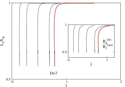
Figure 1: The ratios $L_{e}/L_{p}$ and $R_{2k+1}^{(in)}/R_{2k+1}^{(out)}$, which encode the deformation of the horizon, are shown $vs.$ the reduced angular momentum $j$ for $D=5,6$ black ring solutions and $D=7$ charged black ringoids in EMd theory. The red curves corresponds to the vacuum solutions. The other curves are for charged solutions with the boosting parameters (from right to left) $\alpha=0.5,1,1.5$ and $2$.

For both the MP BHs and $D=5$ BR seed solutions, it is straightforward to write down the corresponding closed form EMd generalizations. For example, in the MP case one replaces in (27)-(28) the following expression of the vacuum seed configuration [1]:

$$f_{0}^{(0)}=\frac{\Delta(r)}{(r^{2}+a^{2})P(r,\theta)},~{}~{}f_{1}^{(0)}=\frac{r^{2}+a^{2}\cos^{2}\theta}{\Delta(r)},~{}~{}f_{2}^{(0)}=r^{2}\cos^{2}\theta,$$

$$f_{3}^{(0)}=(r^{2}+a^{2})\sin^{2}\theta P(r,\theta),~{}~{}f_{4}^{(0)}=(r^{2}+a^{2})\sin^{2}\theta,~{}~{}$$ (29)

$$W^{(0)}=\frac{M}{r^{D-(2k+5)}}\frac{a}{(r^{2}+a^{2})^{k+1}(r^{2}+a^{2}\cos^{2}\theta)P(r,\theta)}~{},$$

$M,a$ being two input parameters and

$$\Delta(r)=(r^{2}+a^{2})\left(1-\frac{M}{r^{D-(2k+5)}(r^{2}+a^{2})^{k+1}}\right),~{}P(r,\theta)=1+\frac{M}{r^{D-(2k+5)}}\frac{a^{2}\sin^{2}\theta}{(r^{2}+a^{2})^{k+1}(r^{2}+a^{2}\cos^{2}\theta)},$$

     

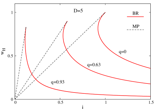
Figure 2: The reduced area $a_{H}$, the reduced temperature $t_{H}$ and the reduced angular velocity $w_{H}$ are shown $vs.$ the reduced angular momentum $j$ for $D=5$ charged black rings (BR) and Myers-Perry (MP) black holes.

where a different choice for $\Delta$ is employed.

Having derived the expressions of the geometry and matter functions, it is straightforward to study all properties of the solutions. For example, in Figure 1 we show the quantities $L_{e}/L_{p}$ and $R_{2k+1}^{(in)}/R_{2k+1}^{(out)}$ which encode the deformation of the horizon (see (16), (17)) for $D=5,6,7$ black ring(oid)s and several values of the boosting parameter $\alpha$. One can see that the charged solutions share the pattern of the neutral ones, being shifted to smaller values of $j$. For example, in the $D=5$ case, the hole inside the ring shrinks to zero size while the outer radius goes to infinity as a critical configuration is approached.

Moreover, for both closed form and numerical solutions, the quantities which enter the first law result from those of the corresponding vacuum seed configurations. A direct computation leads to

     

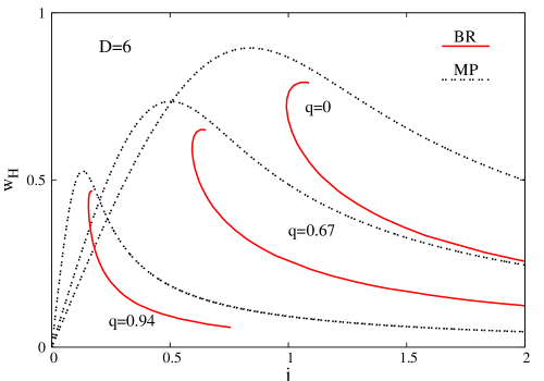
Figure 3: Same as Figure 2 for $D=6$ dimensions.

$${\cal M}=\left(1+\frac{D-3}{D-2}\sinh^{2}\alpha\right){\cal M}^{(0)},~{}~{}J=\cosh\alpha~{}J^{(0)},~{}~{}\Omega_{H}=\frac{1}{\cosh\alpha}\Omega_{H}^{(0)}~{},$$ (30)

$$T_{H}=\frac{1}{\cosh\alpha}T_{H}^{(0)},~{}~{}A_{H}=\cosh\alpha~{}A_{H}^{(0)},~{}~{}Q_{E}=\frac{D-3}{D-2}\sinh\alpha\cosh\alpha~{}{\cal M}^{(0)},~{}~{}\Phi_{H}=\tanh\alpha,$$

and

$$j=\left(\frac{D-2}{D-2+(D-3)\sinh^{2}\alpha}\right)^{\frac{D-2}{D-3}}\cosh\alpha~{}j^{(0)},~{}a_{H}=\left(\frac{D-2}{D-2+(D-3)\sinh^{2}\alpha}\right)^{\frac{D-2}{D-3}}\cosh\alpha~{}a_{H}^{(0)},~{}~{}$$

$$t_{H}=\left(1+\frac{(D-3)}{(D-2)}\sinh^{2}\alpha\right)^{\frac{1}{D-3}}\frac{1}{\cosh\alpha}t_{H}^{(0)},~{}~{}w_{H}=\left(1+\frac{(D-3)}{(D-2)}\sinh^{2}\alpha\right)^{\frac{1}{D-3}}\frac{1}{\cosh\alpha}w_{H}^{(0)},$$ (31)

$$q=\frac{(D-3)\sinh\alpha\cosh\alpha}{D-2+(D-3)\sinh^{2}\alpha}~{},$$

for the scaled variables.

     

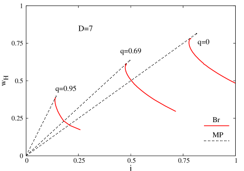
Figure 4: Same as Figure 2 for charged black ringoids (Br) and Myers-Perry (MP) black holes in $D=7$ dimensions (both with 2 equal magnitude angular momenta).

One can see that the boosting parameter $\alpha$ is a monotonic function of the horizon electrostatic potential $\Phi_{H}$ (or, equally, is uniquely fixed by the reduced charge $q$). Also, given a mass ${\cal M}$, the electric charge $Q_{E}$ cannot be arbitrarily large, with $q\leq 1$. The limit $\alpha\to\infty$ corresponds to singular black objects, with $j\to 0$, $a_{H}\to 0$ and $q\to 1$. Moreover, one can show that the Gibbs potential of the charged solutions equals that of the seed vacuum configurations $G=G^{(0)}$, while $F=F^{(0)}+\frac{D-3}{D-2}\sinh^{2}\alpha{\cal M}^{(0)}$.

It follows that, for any finite $\alpha$, some basic thermodynamic properties of these EMd solutions are qualitatively similar to the vacuum seed case. For example, as shown in Figures 2-4, the $(j,a_{H})$ and $(j,t_{H})$ diagrams of the charged solutions have the same shape for any value of $q$. However, the curves in the phase diagram get shifted to lower $a_{H}$ and $j$ as the charge parameter $q$ is increased.

Also, a generic property of the solutions is the occurrence of a cusp in the $a_{H}(j)$ black ring(oid) diagram, where a branch of “fat” black ring(oid) solutions emerges, with the existence of a minimally spinning solution. A comparison of the results (with the set of MP-like solutions included), suggest that, similar to the vacuum case, the $k\geq 1$ black ringoids with $S^{2}\times S^{2k+1}$ horizon topology are the natural counterparts of the $D=5$ BRs. As noticed in [21], the branch of “fat” $D=5$ charged BRs ends in a limiting singular solution with $a_{H}=0$ and nonzero $j$. The same configuration is also approached by the charged MP BHs with maximal $j$. The existing data strongly suggest that this is the picture also for the $D=7$ charged Br and MP solutions.

     

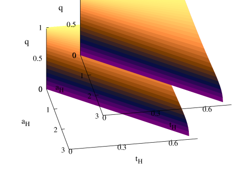
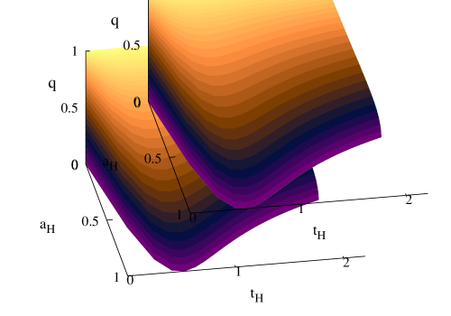
Figure 5: The (area-temperature-charge) diagram is shown for charged Myers-Perry black holes (left) and black rings (right) in $D=5$ dimensions. All quantities are normalized with respect to the mass of the black objects.

     

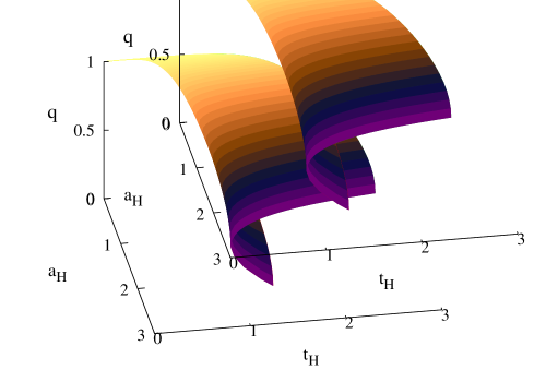
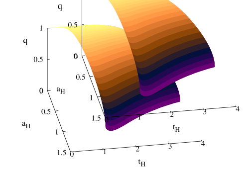
Figure 6: Same as Figure 5 for $D=6$ solutions.

However, a different pattern is found for $D=6$ solutions. There the charged “fat” BRs exhibit a different limiting behaviour; similar to the vacuum case, they end in a critical merger configuration [4], where a branch of “pinched” BHs is approached in a horizon topology changing transition. The results in [6] together with (27), (28) show that the critical merger EMd solution has a finite, nonzero area, while the temperature stays also finite and nonzero.

The (area-temperature-charge) diagram of the MP, BRs and black ringoids is shown in Figures 5-7 (in principle, the equation of state $T(A_{H},Q_{E})$ can be deduced from there). One can notice that the five dimensional case is special, since, as $q\to 1$, $t_{H}\to t_{H}^{(0)}\geq 0$ for $D=5$, while $t_{H}\to 0$ for $D>5$.

     

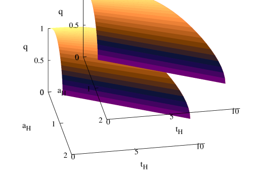
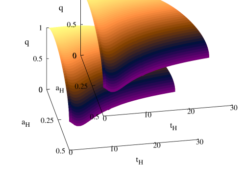
Figure 7: Same as Figure 5 for $D=7$ charged Myers-Perry black holes (left) and black ringoids (right).

Finally, let us mention that, for any event horizon topology, the gyromagnetic ratio (23) has a remarkable simple expression in terms of $\alpha$ only,

$$g=D-3+\frac{1}{\cosh^{2}\alpha},$$ (32)

and varies between $D-3$ (for maximally charged solutions $q=1$, $i.e.$ $\alpha\to\infty$) and $D-2$ (for solutions with an infinitesimally small charge $q\to 0$, $i.e.$ $\alpha\to 0$).

4 Further remarks

Fifteen years after the discovery of the BR by Emparan and Reall [2], [3], the study of BHs with a non-spherical horizon topology continues to be a source of excitement in higher dimensional General Relativity. However, most of the black objects with a nonspherical horizon topology studied in the literature describe vacuum configurations only. Moreover, it is worth noticing that even for the case of an event horizon with spherical topology very few solutions with matter fields are known in closed form (for example, the higher dimensional generalization of the Kerr-Newman solution is only known numerically [17], [25], [26], [27]).

The main purpose of this work was to generalize the non-perturbative framework used in [1] for the study of several classes of vacuum black objects with $k+1$ equal angular momenta, to the case of Einstein-Maxwell-dilaton theory. Our results show that, similar to the pure Einstein gravity case, for general dilaton coupling constant the problem reduces to solving a set of coupled PDEs with suitable boundary conditions on a rectangular domain, employing an adequate numerical scheme [1].

As a preliminary step before considering the generic case, we have studied solutions of EMd theory with the Kaluza-Klein value of the dilaton coupling constant. In this special limit, the action in $D$ dimensions is obtained by reducing the $D+1$ dimensional vacuum Einstein action, while the solutions are found by embedding the $D$ dimensional vacuum solutions in $D+1$ dimensions and boosting in the extra direction.

The resulting EMd solutions are asymptotically flat, and either possess a regular horizon of spherical topology (and thus represent charged generalizations of MP BHs), or an $S^{n+1}\times S^{2k+1}$ topology (and thus represent charged BRs and black ringoids). These black objects are characterized by their global charges: their mass, their $k+1$ equal magnitude angular momenta, and their electric charge.

As mentioned above, these results were obtained only for a particular value of the dilaton coupling constant. It remains a challenge to generalize such solutions to arbitrary values of the dilaton coupling constant, including the pure Einstein-Maxwell case. The construction of more general configurations ($e.g.$ higher dimensional generalizations of the $D=5$ dipole BRs [29], solutions with a Chern-Simons term or black objects coupled with a $p-$form field (with $p>2$)) is another important open question, just like the inclusion of a cosmological constant. We hope to return elsewhere with a systematic study of these aspects.

References

- [1] B. Kleihaus, J. Kunz and E. Radu, JHEP 1501 (2015) 117 [arXiv:1410.0581 [gr-qc]].
- [2] R. Emparan and H. S. Reall, Phys. Rev. Lett. 88 (2002) 101101 [arXiv:hep-th/0110260].
- [3] R. Emparan and H. S. Reall, Phys. Rev. D 65 (2002) 084025 [arXiv:hep-th/0110258].
- [4] R. Emparan, T. Harmark, V. Niarchos, N. A. Obers and M. J. Rodriguez, JHEP 0710 (2007) 110 [arXiv:0708.2181 [hep-th]].
- [5] B. Kleihaus, J. Kunz and E. Radu, Phys. Lett. B 718 (2013) 1073 [arXiv:1205.5437 [hep-th]].
- [6] Ó. J. C. Dias, J. E. Santos and B. Way, JHEP 1407 (2014) 045 [arXiv:1402.6345 [hep-th]].
- [7] R. C. Myers and M. J. Perry, Annals Phys. 172 (1986) 304.
- [8] R. P. Kerr, Phys. Rev. Lett. 11 (1963) 237.
- [9] B. Kleihaus and J. Kunz, arXiv:1603.07267 [gr-qc].
- [10] H. S. Reall, Int. J. Mod. Phys. D 21 (2012) 1230001 [arXiv:1210.1402 [gr-qc]].
- [11] R. Emparan and H. S. Reall, Living Rev. Rel. 11 (2008) 6 [arXiv:0801.3471 [hep-th]].
- [12] R. Emparan and H. S. Reall, Class. Quant. Grav. 23 (2006) R169 [hep-th/0608012].
- [13] B. Kleihaus, J. Kunz and K. Schnülle, Phys. Lett. B 699 (2011) 192 [arXiv:1012.5044 [hep-th]].
- [14] B. Kleihaus, J. Kunz and E. Radu, Phys. Lett. B 723 (2013) 182 [arXiv:1303.2190 [gr-qc]].
- [15] B. Kleihaus, J. Kunz and E. Radu, Phys. Lett. B 678 (2009) 301 [arXiv:0904.2723 [hep-th]].
- [16] B. Kleihaus, J. Kunz, E. Radu and M. J. Rodriguez, JHEP 1102 (2011) 058 [arXiv:1010.2898 [gr-qc]].
- [17] J. Kunz, F. Navarro-Lerida and A. K. Petersen, Phys. Lett. B 614 (2005) 104 [gr-qc/0503010].
- [18] J. Kunz, D. Maison, F. Navarro-Lerida and J. Viebahn, Phys. Lett. B 639 (2006) 95 [hep-th/0606005].
- [19] M. M. Caldarelli, R. Emparan and B. Van Pol, JHEP 1104 (2011) 013 [arXiv:1012.4517 [hep-th]].
- [20] H. K. Kunduri and J. Lucietti, Phys. Lett. B 609 (2005) 143 [hep-th/0412153].
- [21] S. Grunau, Phys. Rev. D 90 (2014) 064022 [arXiv:1407.2009 [gr-qc]].
- [22] O. J. C. Dias, P. Figueras, R. Monteiro, J. E. Santos and R. Emparan, Phys. Rev. D 80 (2009) 111701 [arXiv:0907.2248 [hep-th]].
- [23] O. J. C. Dias, P. Figueras, R. Monteiro and J. E. Santos, Phys. Rev. D 82 (2010) 104025 [arXiv:1006.1904 [hep-th]].
- [24] M. Ortaggio and V. Pravda, JHEP 0612 (2006) 054 [gr-qc/0609049].
- [25] J. Kunz, F. Navarro-Lerida and J. Viebahn, Phys. Lett. B 639 (2006) 362 [hep-th/0605075].
- [26] J. L. Blazquez-Salcedo, J. Kunz and F. Navarro-Lerida, Phys. Lett. B 727 (2013) 340 [arXiv:1309.2088 [gr-qc]].
- [27] J. L. Blazquez-Salcedo, J. Kunz and F. Navarro-Lerida, Phys. Rev. D 89 (2014) 024038 [arXiv:1311.0062 [gr-qc]].
- [28] A. Sen, Nucl. Phys. B 440 (1995) 421 [arXiv:hep-th/9411187].
- [29] R. Emparan, JHEP 0403 (2004) 064 [hep-th/0402149].