String order via Floquet interactions in atomic systems
Abstract
We study the transverse-field Ising model with interactions that are modulated in time. In a rotating frame, the system is described by a time-independent Hamiltonian with many-body interactions, similar to the cluster Hamiltonians of measurement-based quantum computing. In one dimension, there is a three-body interaction, which leads to string order instead of conventional magnetic order. We show that the string order is robust to power-law interactions that decay with the cube of distance. In two and three dimensions, there are five- and seven-body interactions. We discuss adiabatic preparation of the ground state as well as experimental implementation with trapped ions, Rydberg atoms, and polar molecules.
I Introduction
A current goal in atomic physics is to realize exotic many-body phases, since atomic-physics experiments can simulate the physics of condensed-matter systems Pachos and Plenio (2004); Bermudez et al. (2009); Gorshkov et al. (2011); Lee et al. (2013); Yan et al. (2013); Richerme et al. (2014); Cohen and Retzker (2014); Daley and Simon (2014); Chan et al. (2015); Schauß et al. (2015); Gong et al. (2016); Kaczmarczyk et al. . An advantage of atomic quantum simulators is that they are highly tunable. For example, the interaction between atoms is often induced by a laser, so one can easily tune the interaction strength, sign, and range by changing the laser parameters Mølmer and Sørensen (1999); Porras and Cirac (2004).
An intriguing type of many-body phase is symmetry-protected topological order Chen et al. (2011). A common feature of such a phase is string order. A system with string order does not appear to have long-range order according to two-site correlation functions. However, if one calculates a nonlocal correlation function involving a long “string” of operators, the hidden order becomes apparent. A well-known example of string order is the Haldane phase of a spin-1 chain Haldane (1983); den Nijs and Rommelse (1989); Kennedy and Tasaki (1992); Else et al. (2013).
In this paper, we show that one can realize string order with spin-1/2 particles by modulating the interaction of the transverse-field Ising model. This scheme is well-suited for atomic-physics experiments, since it exploits their tunability. In one-dimension, a spin chain with time-modulated, two-body interactions is equivalent to a spin chain with time-independent, three-body interactions. The three-body interaction leads to string order in the ground state. The three-body interaction is a cluster Hamiltonian of measurement-based quantum computing, and the string order is a manifestation of the cluster phase Raussendorf and Briegel (2001); Nielsen (2006). We discuss how to adiabatically prepare the ground state in the laboratory frame.
We then show that the scheme works even if the original spin chain has power-law interactions, as is common in atomic-physics experiments Yan et al. (2013); Richerme et al. (2014); Schauß et al. (2015); Gong et al. (2016). For interactions that decay with the cube of distance, the long-range interactions have negligible effect on the ground state, and the ground state still has string order. We also show that modulating the interaction in two and three dimensions leads to five- and seven-body interactions. Finally, we discuss experimental implementation with trapped ions, Rydberg atoms, and polar molecules.
In recent years, there has been a lot of work on using time-periodic modulation to control many-body systems (see Refs. Bukov et al. (2015); Eckardt for recent reviews). The generation of many-body interactions has been previously studied in the context of bosonic quantum gases Gong et al. (2009); Rapp et al. (2012); Greschner et al. (2014); Meinert et al. (2016) and spin models Engelhardt et al. (2013); Iadecola et al. (2015). Other time-modulated spin models have also been studied Bastidas et al. (2012); Russomanno and Torre ; Gómez-León and Stamp .
II General model
We consider a lattice of spin-1/2 particles, where the spin-spin interaction is modulated in time. The Hamiltonian is ()
| (1) |
where are the Pauli matrices for spin , is the modulation amplitude, and is the transverse field strength. The 1/2 accounts for double-counting pairs in the sum. For now, we let the lattice be arbitrary, and encodes the connectivity between spins and . In later sections, we will consider one, two, and three-dimensional lattices. Reference Engelhardt et al. (2013) studied the case of all-to-all coupling. Reference Iadecola et al. (2015) studied the case of one dimension with nearest-neighbor interactions.
For convenience, we define the operator , which is the sum of the spins that spin interacts with. Then Eq. (1) can be written as
| (2) |
To analyze this time-dependent model, we use Floquet theory Bukov et al. (2015); Eckardt . We go into the interaction picture, rotating with the first term of Eq. (2). In this rotating frame, becomes :
| (3) | |||||
| (4) | |||||
| (5) |
Then we use the Baker-Campbell-Hausdorff formula to rewrite ,
We write in terms of Bessel functions:
| (8) |
is still time dependent, so we make a rotating-wave approximation Ashhab et al. (2007); Bastidas et al. (2012). The terms in oscillate very quickly and are off-resonant. Thus, we only need to keep the terms to capture the slow-time-scale dynamics. This rotating-wave approximation is valid when
| (9) |
So the final Hamiltonian is
| (10) | |||||
| (11) |
Thus, in the interaction picture and when is sufficiently large, the system is described by the time-independent Hamiltonian in Eq. (11). At this point, we choose a lattice geometry () and expand in a power series:
| (12) |
We obtain arbitrary even powers of , which can be simplified using the fact that . In general, has many-body interactions involving one and an even number of ’s, e.g., . is reminiscent of cluster Hamiltonians that arise in measurement-based quantum computing Raussendorf and Briegel (2001); Nielsen (2006).
The presence of many-body interactions in can be intuitively understood as follows. The transverse field in causes spin to undergo Rabi oscillations between and . However, the modulated interaction means that spin sees an oscillating energy shift that depends on its neighbors’ . Similarly, the many-body terms in mean that spin Rabi-oscillates depending on its neighbors’ , but now the energy shift is time-independent.
The relationship between the wave function in the laboratory frame (evolving with ) and the wave function in the rotating frame (evolving with ) is:
| (13) |
Equations (4) and (5) say that when is a multiple of , and . Thus, if we measure the system at these periodic times, and we do not have to worry about converting between the two frames Engelhardt et al. (2013).
There is a simple way to convert between the two frames at arbitrary times. We note that , where is the evolution operator of with and . Thus, after we have obtained , if we evolve it further for time with and , we obtain .
In Eq. (1), we assumed that the interaction alternates sign, but our results still hold if the interaction is modulated without changing sign. In that case, is the same, but is different Bastidas et al. (2012). In some experimental setups, it is easier to modulate the strength without changing the sign.
Lastly, we note that although we assume spin-1/2 in this paper, one obtains similar results for higher spin. Suppose the in Eq. (1) were for higher spin. Then would still be given by Eq. (11), since the commutation relations of do not depend on the spin magnitude. The difference is that for higher spin, so the expanded and simplified form of would look different.
III One dimension with nearest-neighbor interactions
III.1 Model
We now consider a one-dimensional lattice of spins with nearest-neighbor interactions, which was first studied in Ref. Iadecola et al. (2015). We assume open boundary conditions. However, we add a longitudinal field to the edge spins:
It is not necessary to add , but without these extra terms, the ground state of is fourfold degenerate due to a symmetry Iadecola et al. (2015); Son et al. (2011); Smacchia et al. (2011). Although this degeneracy is a signature of symmetry-protected-topological order, it is problematic if one wants to adiabatically prepare the ground state of ; without these terms, one needs a slower ramp. Another reason for adding these terms is to make look more like a cluster Hamiltonian, as discussed below.
The non-edge spins have , while the edge spins have and . After expanding and simplifying Eq. (11), we obtain Iadecola et al. (2015)
| (15) | |||||
| (16) | |||||
| (17) |
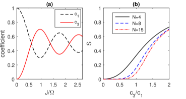
Thus, has a transverse field with strength and a three-body interaction with strength . The ratio can be adjusted by varying [Fig. 1(a)]. The transverse field is always present, although it can be weaker than the three-body interaction. reaches its maximum value of 2.35 when .
III.2 Cluster phase
in Eq. (15) is significant for two reasons. First, the terms in parentheses are a cluster Hamiltonian Pachos and Plenio (2004); Doherty and Bartlett (2009); Skrøvseth and Bartlett (2009); Son et al. (2011); Smacchia et al. (2011); Giampaolo and Hiesmayr (2015). The (unique) ground state of a cluster Hamiltonian is a cluster state, which is a highly entangled state that is useful for measurement-based quantum computing Raussendorf and Briegel (2001); Nielsen (2006). Note that in order to be a cluster Hamiltonian, must have boundary terms as in Eq. (15), which is why we included in Eq. (LABEL:eq:H_1d).
is also significant because the ground state exhibits a phase transition to string order. The string-order parameter is Son et al. (2011); Smacchia et al. (2011); Giampaolo and Hiesmayr (2015)
| (18) |
although other string-order parameters also work Doherty and Bartlett (2009); Skrøvseth and Bartlett (2009). When , the ground state has string order (), and the system is in the “cluster phase,” since the ground state is still useful for measurement-based quantum computing even if Doherty and Bartlett (2009). When , the ground state is in the paramagnetic phase (). The critical point at is a second-order phase transition. These properties can be obtained analytically by using the Jordan-Wigner transformation Pachos and Plenio (2004); Smacchia et al. (2011) or by mapping to the (time-independent) transverse-field Ising model Doherty and Bartlett (2009); Son et al. (2011). Note that two-site correlations, such as , do not show long-range order Pachos and Plenio (2004).
There is in fact a deep connection between string order and measurement-based quantum computing Doherty and Bartlett (2009). In measurement-based quantum computing, one does a sequence of local measurements to entangle distant qubits. The sequence of local measurements is equivalent to a string operator. If a state’s string-order parameter is nonzero, the state is useful for measurement-based quantum computing because local measurements on it produce a state that is more entangled than a random state. A larger string-order parameter implies more usefulness.
Figure 1(b) shows the string-order parameter for finite , calculated using exact diagonalization of . As increases, the phase transition at becomes more evident.
III.3 Adiabatic preparation
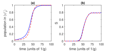
Now we discuss how to adiabatically prepare the cluster phase of by turning on the three-body interaction. We linearly increase from 0 to over a time , such that starts at 0 and ends at the maximum value of 2.35. The phase transition at corresponds to . The system starts in , which is the initial paramagnetic ground state of . We denote the final ground state of as , which is the desired cluster phase.
We first simulate the adiabatic ramp in the rotating frame ( evolves with ). Figure 2 shows there is a clean transfer of population into , as expected. There is a slight infidelity, which can be reduced by using a slower ramp (larger ).
Next, we simulate the adiabatic ramp in the laboratory frame ( evolves with ). We sample at periodic times, so that the wave functions of the laboratory and rotating frames coincide. Figure 2(a) shows that the population transfer in the laboratory frame is similar to the rotating frame. The deviation is due to the rotating-wave approximation, but the agreement improves as increases. Interestingly, despite the deviation from during the ramp, ends up in with very high fidelity.
In Fig. 2(b) we plot the string-order parameter as a function of time. As expected, starts at zero and ends at a nonzero value.
It turns out that this adiabatic method does not work for , due to a symmetry of . If one starts the adiabatic ramp in , the system ends up in an excited state.
IV One dimension with power-law interactions
We now consider a one-dimensional lattice with power-law interactions, i.e., the spin-spin interaction decreases with a power law in distance (). The motivation is that atom-based quantum simulators (e.g., trapped ions Richerme et al. (2014), Rydberg atoms Schauß et al. (2015), and polar molecules Gorshkov et al. (2011)) usually have power-law interactions. Below, we present results for , which are relevant to these experiments. We show that is almost identical to the nearest-neighbor model, whereas is quite different.
IV.1 Model
We assume open boundary conditions and again add a longitudinal field to the edge spins:
| (19) | |||||
So for non-edge spins, .
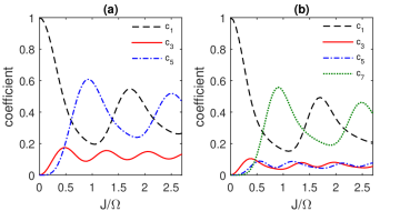
We now calculate for Eq. (19). Since now has coupling between every pair of spins, has many more terms than Eq. (15). There are three-body terms between non-neighboring spins. There are also many-body interactions involving five, seven, etc., spins. There are two questions we seek to answer. First, how large are these extra terms? Second, how does the ground state of the new compare to that of the nearest-neighbor case [Eq. (15)]?
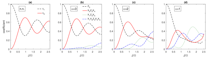
To get a sense of the magnitude of the extra terms, we consider in detail the case of spins, which is representative of larger . In this case, has one-, three-, and five-body terms. Figure 3 plots the coefficients for some terms that involve . We calculated these coefficients numerically by expanding Eq. (11) to sufficient order. We see that the extra terms are small for but large for . So for is very similar to the nearest neighbor case, whereas is quite different.
We discuss in detail the case of . For , the coefficients of and are very close to Eqs. (16) and (17), whereas the coefficients of the extra terms are small. If we set (which maximized for the nearest-neighbor case), the extra terms are very small. The largest extra term is , whose coefficient is still 1/30 that of . Also, the new three-body terms are smaller than what one would naively expect based on the cubic power law. For example, one would expect the coefficient of to be that of (since the and interactions in are 1/8 those of and ), but the ratio is actually . So the power-law decay of interaction in does not directly carry over to .
Although Fig. 3 only shows terms involving , we observe similar behavior for other . Furthermore, as we increase , the above observations still hold. So for is very close to that for the nearest neighbor case [Eq. (15)]. However, it is possible that the ground states are very different, so we proceed to compare the ground states.
IV.2 Ground state of
Here, we compare the ground state of for the power-law case with the ground state of for the nearest-neighbor case [Eq. (15)]. In principle, we could find by first calculating all terms of via Eq. (11), then diagonalizing to find the ground state, but this is very tedious for large . A more convenient way is to perform an adiabatic ramp of , such as in Sec. III.3: If the ramp is very slow (to ensure adiabaticity) and is very large (to validate the rotating-wave approximation), then will be prepared with very high fidelity. (At the moment, we are interested in the ideal case in order to obtain the ground state of . In Sec. VI.2, we will use more realistic experimental parameters.) Note that, as discussed in Sec. III.3, the ground states for , are inaccessible via adiabatic ramp.
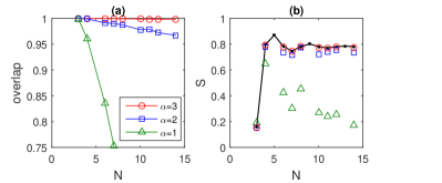
Figure 4 compares with for . In these plots, was obtained using and . Figure 4(a) shows the overlap for different and . The case of has very high overlap (0.998 for ), whereas the case of has small overlap. Actually, the overlap is larger than what is plotted due to the way we obtained , i.e., using a slower ramp and larger would make the overlap even higher. Figure 4(b) plots the string-order parameter : For , there is very good agreement between and . Thus for , is almost identical to . This means that quantum simulators with cubic power-law interactions can observe the transition to string order.
V Higher dimension
Now we consider two- and three-dimensional square lattices with nearest-neighbor interactions,
| (20) |
For simplicity, we assume periodic boundary conditions.
For a 2D lattice, expanding Eq. (11) leads to
| (21) | |||||
| (22) | |||||
| (23) | |||||
| (24) |
where denotes the nearest neighbors of spin , and means to include each set of neighbors only once. The terms are three-body interactions involving each pair of neighbors of , whereas the terms are five-body interactions involving all four neighbors. Figure 5(a) plots the coefficients. There are ranges of where .
Equation (21) was previously studied for the case of Doherty and Bartlett (2009). There is a phase transition at with string order for , where the string runs diagonally across the lattice. Note from Fig. 5(a) that always has ; it will be interesting to see how affects the phase transition described in Ref. Doherty and Bartlett (2009).
For a 3D lattice, expanding Eq. (11) leads to
| (25) | |||||
So includes up to seven-body interactions. Figure 5(b) plots the coefficients. There are ranges of where .
It is important to note that in Eq. (24) and in Eq. (V) are the same order as in Eq. (17). This is surprising since one would expect interactions involving more spins to be a lot smaller. We also note that Eqs. (21) and (25) are cluster Hamiltonians; this is significant because a measurement-based quantum computer beats a classical computer when the cluster state is on a lattice higher than 1D Nielsen (2006).
It turns out that the form and coefficients of depend only on the number of neighbors in . If was on a 2D triangular lattice (six neighbors), would still be given by Eqs. (25)–(V). This is because has the same form for a 2D triangular lattice as a 3D square lattice. On the other hand, a 2D honeycomb lattice (three neighbors) would have a different form.
VI Experimental implementation
VI.1 Possible setups
We now discuss three types of experiments that could modulate the interaction as in Eq. (1). In these experiments, a spin state is encoded in the levels of an atom or molecule, and the spin-spin interaction is engineered via laser fields. Time-independent interactions have been demonstrated for all three types, and introducing a modulation is straightforward. (It is easier to modulate the interaction strength without changing the sign, but our results still hold in this case, albeit with a different Bastidas et al. (2012).) These experiments have power-law interactions, but Sec. IV showed that ends up being very similar to the nearest-neighbor case.
The first example is trapped ions Richerme et al. (2014). In this setup, a laser induces a spin-spin interaction between ions (0–3). The sign and magnitude of the interaction depends on the frequency and intensity of the laser Mølmer and Sørensen (1999); Porras and Cirac (2004). By modulating the laser parameters, one modulates the interaction.
The second example is Rydberg atoms Schauß et al. (2015). Rydberg levels have strong polar interactions. One can generate spin-spin interactions () by dressing a ground state with a Rydberg state via an off-resonant laser Macrì and Pohl (2014). The sign and magnitude of the interaction depends on which Rydberg state is used and the intensity of the dressing laser. By modulating the intensity of the dressing laser, one modulates the interaction. An alternative approach is to directly populate a Rydberg state; since the polar interaction can be tuned via a Förster resonance Barredo et al. (2015), one can modulate the interaction by modulating electric or microwave fields.
The third example is polar molecules Gorshkov et al. (2011); Yan et al. (2013). In this case, a spin is encoded in the rotational degree of freedom of a molecule. The molecules interact via polar interactions (), which can be tuned via electric and microwave fields. By modulating the latter, one modulates the interaction.
VI.2 Experimental numbers
To maximize fidelity of the prepared ground state, and should both be large to ensure validity of the rotating-wave approximation and adiabaticity, respectively. In practice, these are limited because the interaction strength cannot be arbitrarily large and the system has a finite coherence time.
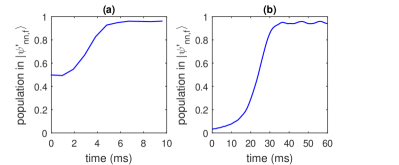
We give example numbers for trapped ions. Recent experiments have implemented a spin chain with power-law interactions with Richerme et al. (2014). We simulate a 1D chain with [Eq. (19)] and increase linearly from 0 to over a time . We set to maximize the final three-body interaction. The rotating-wave approximation requires ; empirically, we obtain reasonable results with , which corresponds to
The required increases with . For , is sufficient to prepare the ground state of with reasonably high fidelity [Fig. 6(a)]. This is on the order of the coherence time of current experiments Richerme et al. (2014). For , is sufficient [Fig. 6(b)]. One could decrease by increasing the maximum or by optimizing the ramp profile.
VII Modulated interactions
We briefly discuss the effect of time modulation on the chain,
| (30) |
For simplicity, we assume one dimension, nearest-neighbor interactions, and periodic boundary conditions. Such a model can also be implemented with trapped ions, since the and interactions can be independently controlled, although the interaction would be long range Porras and Cirac (2004).
By going into the interaction picture and taking the rotating-wave approximation as in Sec. II, we obtain a time-independent Hamiltonian,
| (31) | |||||
| (32) | |||||
| (33) |
contains two- and four-body interactions, where and are exactly the same as and in Eqs. (16) and (17). Equation (31) has been shown to have a second-order phase transition from antiferromagnetic order () to nematic order () Giampaolo and Hiesmayr (2015), where the latter is also characterized by a nonlocal order parameter.
VIII Conclusion
We have presented a simple method of generating many-body interactions in atomic systems. One future direction is to consider the effect of disorder. It is known that the transverse-field Ising model with quenched disorder forms a Griffiths phase Fisher (1992); Iglói and Monthus (2005). It would be interesting to see if the Griffiths phase survives time modulation of the interaction.
Another direction is to add a second slower modulation. For example, suppose one modulated in Eq. (15) by modulating on a slower time scale than . By going into another rotating frame, one may obtain an even more exotic spin chain.
Acknowledgements.
The simulations in this paper were performed on Indiana University’s supercomputer, Big Red II. Y.N.J. was supported by NSF-DMR Grant No. 1054020.References
- Pachos and Plenio (2004) J. K. Pachos and M. B. Plenio, Phys. Rev. Lett. 93, 056402 (2004).
- Bermudez et al. (2009) A. Bermudez, D. Porras, and M. A. Martin-Delgado, Phys. Rev. A 79, 060303 (2009).
- Gorshkov et al. (2011) A. V. Gorshkov, S. R. Manmana, G. Chen, J. Ye, E. Demler, M. D. Lukin, and A. M. Rey, Phys. Rev. Lett. 107, 115301 (2011).
- Lee et al. (2013) T. E. Lee, S. Gopalakrishnan, and M. D. Lukin, Phys. Rev. Lett. 110, 257204 (2013).
- Yan et al. (2013) B. Yan, S. A. Moses, B. Gadway, J. P. Covey, K. R. Hazzard, A. M. Rey, D. S. Jin, and J. Ye, Nature 501, 521 (2013).
- Richerme et al. (2014) P. Richerme, Z.-X. Gong, A. Lee, C. Senko, J. Smith, M. Foss-Feig, S. Michalakis, A. V. Gorshkov, and C. Monroe, Nature 511, 198 (2014).
- Cohen and Retzker (2014) I. Cohen and A. Retzker, Phys. Rev. Lett. 112, 040503 (2014).
- Daley and Simon (2014) A. J. Daley and J. Simon, Phys. Rev. A 89, 053619 (2014).
- Chan et al. (2015) C.-K. Chan, T. E. Lee, and S. Gopalakrishnan, Phys. Rev. A 91, 051601 (2015).
- Schauß et al. (2015) P. Schauß, J. Zeiher, T. Fukuhara, S. Hild, M. Cheneau, T. Macrì, T. Pohl, I. Bloch, and C. Gross, Science 347, 1455 (2015).
- Gong et al. (2016) Z.-X. Gong, M. F. Maghrebi, A. Hu, M. Foss-Feig, P. Richerme, C. Monroe, and A. V. Gorshkov, Phys. Rev. B 93, 205115 (2016).
- (12) J. Kaczmarczyk, H. Weimer, and M. Lemeshko, arXiv:1601.00646 .
- Mølmer and Sørensen (1999) K. Mølmer and A. Sørensen, Phys. Rev. Lett. 82, 1835 (1999).
- Porras and Cirac (2004) D. Porras and J. I. Cirac, Phys. Rev. Lett. 92, 207901 (2004).
- Chen et al. (2011) X. Chen, Z.-C. Gu, and X.-G. Wen, Phys. Rev. B 83, 035107 (2011).
- Haldane (1983) F. Haldane, Phys. Lett. A 93, 464 (1983).
- den Nijs and Rommelse (1989) M. den Nijs and K. Rommelse, Phys. Rev. B 40, 4709 (1989).
- Kennedy and Tasaki (1992) T. Kennedy and H. Tasaki, Phys. Rev. B 45, 304 (1992).
- Else et al. (2013) D. V. Else, S. D. Bartlett, and A. C. Doherty, Phys. Rev. B 88, 085114 (2013).
- Raussendorf and Briegel (2001) R. Raussendorf and H. J. Briegel, Phys. Rev. Lett. 86, 5188 (2001).
- Nielsen (2006) M. A. Nielsen, Rep. Math. Phys. 57, 147 (2006).
- Bukov et al. (2015) M. Bukov, L. D’Alessio, and A. Polkovnikov, Adv. Phys. 64, 139 (2015).
- (23) A. Eckardt, arXiv:1606.08041 .
- Gong et al. (2009) J. Gong, L. Morales-Molina, and P. Hänggi, Phys. Rev. Lett. 103, 133002 (2009).
- Rapp et al. (2012) A. Rapp, X. Deng, and L. Santos, Phys. Rev. Lett. 109, 203005 (2012).
- Greschner et al. (2014) S. Greschner, L. Santos, and D. Poletti, Phys. Rev. Lett. 113, 183002 (2014).
- Meinert et al. (2016) F. Meinert, M. J. Mark, K. Lauber, A. J. Daley, and H.-C. Nägerl, Phys. Rev. Lett. 116, 205301 (2016).
- Engelhardt et al. (2013) G. Engelhardt, V. M. Bastidas, C. Emary, and T. Brandes, Phys. Rev. E 87, 052110 (2013).
- Iadecola et al. (2015) T. Iadecola, L. H. Santos, and C. Chamon, Phys. Rev. B 92, 125107 (2015).
- Bastidas et al. (2012) V. M. Bastidas, C. Emary, G. Schaller, and T. Brandes, Phys. Rev. A 86, 063627 (2012).
- (31) A. Russomanno and E. G. D. Torre, arXiv:1510.08866 .
- (32) Á. Gómez-León and P. Stamp, arXiv:1512.08315 .
- Ashhab et al. (2007) S. Ashhab, J. R. Johansson, A. M. Zagoskin, and F. Nori, Phys. Rev. A 75, 063414 (2007).
- Son et al. (2011) W. Son, L. Amico, R. Fazio, A. Hamma, S. Pascazio, and V. Vedral, Europhys. Lett. 95, 50001 (2011).
- Smacchia et al. (2011) P. Smacchia, L. Amico, P. Facchi, R. Fazio, G. Florio, S. Pascazio, and V. Vedral, Phys. Rev. A 84, 022304 (2011).
- Doherty and Bartlett (2009) A. C. Doherty and S. D. Bartlett, Phys. Rev. Lett. 103, 020506 (2009).
- Skrøvseth and Bartlett (2009) S. O. Skrøvseth and S. D. Bartlett, Phys. Rev. A 80, 022316 (2009).
- Giampaolo and Hiesmayr (2015) S. M. Giampaolo and B. C. Hiesmayr, Phys. Rev. A 92, 012306 (2015).
- Macrì and Pohl (2014) T. Macrì and T. Pohl, Phys. Rev. A 89, 011402 (2014).
- Barredo et al. (2015) D. Barredo, H. Labuhn, S. Ravets, T. Lahaye, A. Browaeys, and C. S. Adams, Phys. Rev. Lett. 114, 113002 (2015).
- Fisher (1992) D. S. Fisher, Phys. Rev. Lett. 69, 534 (1992).
- Iglói and Monthus (2005) F. Iglói and C. Monthus, Phys. Rep. 412, 277 (2005).