Stability of ion acoustic nonlinear waves and solitons in magnetized plasmas

Abstract

Early results concerning the shape and stability of ion acoustic waves are generalized to propagation at an angle to the magnetic field lines. Each wave has a critical angle for stability. Known soliton results are recovered as special cases. A historical overview of the problem concludes the paper.

1 Introduction

Some time ago the problem of stability of waves described by the Zakharov Kuznetsov equation (ZK, 1974) was solved for arbitrary shape of the wave. Its propagation, however, was limited to clinging to the magnetic field (Infeld 1985). As a check, the soliton case, further limited to perpendicular instabilities, was recovered as found by Laedke and Spatschek (1982). Since then several authors have looked at the propagation and some at stability in various configurations (Infeld and Frycz, 1987 & 1989, Allen and Rowlands, 1993, 1995 & 1997, Munro & Parks 1999, Nawaz et a1 2013, Murawski and Edwin 1992, Bas and Bulent 2010, Mothibi 2015) and several others. Here we present a small $K$ stability analysis of a nonlinear wave propagating at an angle to the magnetic field. Its shape is treated exactly and a cubic is obtained for the frequency of the perturbation (or growth rate). For zero angle, the cubic found in Infeld 1985 is recovered, (see also the book by Infeld and Rowlands 2000). The ZK equation is taken in the form

$$\frac{{\partial}n}{{\partial}t}+\frac{1}{3}\left({\partial}_{x}^{2}+{\partial}_{y}^{2}+3n\right)\frac{{\partial}n}{{\partial}x}=0.$$ (1.1)

Here $x$ is along the uniform field $\boldsymbol{B}$. The wave is propagating at an angle $\theta$ and it proves convenient to rotate the system by this angle. Thus

$$x=\cos\theta\,\xi+\sin\theta\,\eta$$

$$y=\sin\theta\,\xi-\cos\theta\,\eta,$$ (1.2)

and ZK is now

$$\frac{{\partial}n}{{\partial}t}+\left(n+\frac{{\partial}_{\xi}^{2}+{\partial}_{\eta}^{2}}{3}\right)\left(\cos\theta\,n_{\xi}+\sin\theta\,n_{\eta}\right)=0$$ (1.3)

2 Shape of the wave and possible perturbation

We assume the nonlinear wave or soliton to be a function of $\xi-Ut$

We now look for stationary nonlinear solutions of the form

$$n_{0}^{\prime}(\xi^{\prime})=n_{0}+U/\cos\,\theta,\quad\xi^{\prime}=\xi-Ut$$ (2.1)

thus adding a constant to $n_{0}$ which we simply include in zero order. Thus in the new variables, dropping the primes and integrating twice

$$\frac{1}{3}\,{\partial}^{2}_{\xi}n_{0}+\frac{1}{2}n_{0}^{2}=C$$

$$\frac{1}{6}({\partial}_{\xi}n_{0})^{2}=Cn_{0}-\frac{1}{6}n_{0}^{3}+D.$$ (2.2)

By rescaling the variables and the constants we may always reduce the number of parameters putting

$$C=1/6,\quad D(C=1/6)=\zeta/6.$$ (2.3)

To obtain positive

$$n_{0\xi}^{2}=n_{0}-n_{0}^{3}+\zeta$$ (2.4)

in a finite interval of $n_{0}$, the parameter $\zeta$ has to satisfy

$$-2/\sqrt{27}<\zeta<2/\sqrt{27}$$ (2.5)

and the stationary solution $n_{0}(\xi)$ is periodic with a period $\lambda$, which may be defined in terms of complete elliptic integrals.

Suppose a periodic wave solution is perturbed such that the wave vector $\boldsymbol{K}$ of the perturbation forms an angle $\psi$ with the direction $\boldsymbol{\xi}$ of the nonlinear wave. In the coordinate system of the basic wave we have

$$n = n_{0}(\xi)+\delta n=n_{0}(\xi)+\tilde{\delta}n(\xi)e^{i[(K\,\cos\,\psi)\xi+(K\,\sin\,\psi)\eta-\Omega t]}$$ (2.6)

$$\boldsymbol{K} = K\,(\cos\,\psi,~{}\sin\,\psi)$$ (2.7)

and $\tilde{\delta}n(\xi)$ is $\lambda$ periodic. We now assume $K$ small and expand:

$$\Omega = \Omega_{1}(\psi)K+\Omega_{2}(\psi)K^{2}+...$$ (2.8)

$$\tilde{\delta}n = \delta n_{0}+K\delta n_{1}+K^{2}\delta n_{2}+...$$ (2.9)

Consistency in second order will yield a relationship of the form

$$G(\Omega,\boldsymbol{K},\zeta)=0,$$ (2.10)

generalizing a dispersion relation theory.

Introducing

$$L=\frac{1}{3}{\partial}_{\xi}^{2}+n_{0}$$

we find

$${\partial}_{\xi}L\tilde{\delta}n=\frac{1}{3}{\partial}_{\xi}^{3}\tilde{\delta}n+{\partial}_{\xi}n_{0}\tilde{\delta}n=-i\,\Omega\tilde{\delta}n$$

$$-iK\left[\cos\,\theta\,\cos\,\psi\,(n_{0}\tilde{\delta}n+\tilde{\delta}n_{\xi\xi})+\sin\,\theta\,\sin\,\psi\left(n_{0}\tilde{\delta}n+\frac{1}{3}\tilde{\delta}n_{\xi\xi}\right)\right]$$

$$+K^{2}\left[\cos\,\theta\left(\cos^{2}\psi+\frac{1}{3}\sin^{2}\psi\right)+\frac{2}{3}\sin\theta\,\sin\,\psi\,\cos\,\psi\right]\tilde{\delta}n_{\xi}$$ (2.11)

3 Dispersion relation cubic for $\Omega/K$

In second order in $K$, a dispersion relation is obtained.

$$\left(\Omega^{*}/K\right)^{3}+\frac{2}{9}\frac{[4+3Y(Y+6\zeta)](3\cos\psi-\tan\theta\sin\psi)}{Y^{3}-4Y-8\zeta}\left(\Omega^{*}/K\right)^{2}$$

$$+\frac{2}{15}\frac{(Y+3\zeta)(Y^{2}-4/3)(1-5\tan^{2}\theta)\sin^{2}\psi+5[4\zeta+Y(8/3+3Y\zeta)]\sin 2\psi\tan\theta}{Y^{3}-4Y-8\zeta}\left(\Omega^{*}/K\right)$$

$$+\frac{8}{27}\frac{(27\zeta^{2}-4)\cos^{2}\psi(\cos\psi+\sin\psi\tan\theta)}{Y^{3}-4Y-8\zeta}$$

$$+\frac{8}{45}\frac{(Y+3\zeta)^{2}\sin^{2}\psi(\cos\psi+\sin\psi\tan\theta)}{Y^{3}-4Y-8\zeta}=0$$ (3.1)

where $\Omega^{*}=\Omega-UK\sin\psi\tan\theta$. Here $n_{1}$, $n_{2}$, $n_{3}$, are roots of $n_{x}^{2}$ in increasing order. Also $n_{0}$ is contained between $n_{2}$, and $n_{3}$. Other definitions are

$$s=\frac{n_{3}-n_{2}}{n_{3}-n_{1}}\leq 1,\quad Y=2\langle n_{0}\rangle=2\left[n_{1}+(n_{3}-n_{1})\frac{E(s)}{K(s)}\right]$$ (3.2)

$E(s)$ and $K(s)$ are complete elliptic integrals of modulus $s$.

For $\theta=0$ we regain the result of the Infeld and Rowlands book (eq. (8.3.90) in ref. [8]).

We limit further analysis to the most unstable angle of perturbation $\psi=\pi/2$.

There is an instability for $\theta=0$, and $\theta>0$ up to a critical angle. The angle may easily be obtained e.g. by an analysis of the discriminant of the cubic. For $\zeta=0$ ($n_{1}=-1,~{}n~{}_{2}=0,~{}n_{3}=1$), the critical angle is equal $0.792946~{}\mathrm{rad}\approx 45.4325$^∘ (Fig.1).

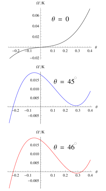
Figure 1: The cubic for $\theta=0,~{}\theta=45$^∘ and $\theta=46$^∘, while $\psi=\pi/2$ . Single $\theta$-intercept means that two roots are complex conjugate; one of them corresponds to the unstable mode. When the cubic has 3 real roots, no instability occurs. The critical angle apparently lies between 45^∘ and 46^∘.

The growth rate $\Gamma/K$ increases from its value at $\theta=0$ to a maximum, then falls to zero at the critical $\theta$ (Fig.2). For all acute angles $\theta$ above the critical one the system is stable to first order in $K$.

For $\theta>\pi/2$ the situation is symmetric with respect to $\theta\rightleftarrows\pi-\theta$.

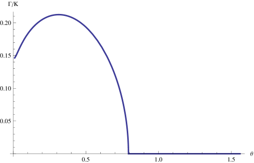
Figure 2: The growth-rate $\Gamma/K$ as a function of $\theta$ for $\zeta=0$. The instability vanishes above the critical angle $\theta\approx 0.793$.

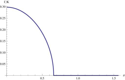
Figure 3: The growth-rate $\Gamma/K$ as a function of $\theta$ for the soliton case $\zeta=2/\sqrt{27}$. The growth-rate decreases from 0.298 at $\theta=0$ to zero at the critical angle $\theta\approx 0.659$.

Another limit of interest is for a soliton propagating at an angle to $\boldsymbol{B}$. For it $\zeta=2/\sqrt{27}$ and the cubic dispersion relation reads

$$(\Omega^{*}/K)^{3}-\frac{\sin\theta}{3\sqrt{3}}(\Omega^{*}/K)^{2}+\frac{4}{45}(\cos^{2}\theta-5\sin^{2}\theta)(\Omega^{*}/K)+\frac{4}{45\sqrt{3}}\cos^{2}\theta\sin\theta=0$$ (3.3)

Here the growth rate is greatest for $\theta=0$, where it is equal $2/(3\sqrt{5})\approx 0.298142$. Then it decreases to zero at the critical angle, which is $\mathrm{arctan}\sqrt{3/5}\approx 0.659058~{}\mathrm{rad}\approx 37.7612$^∘(Fig.3), in agreement with Allen and Rowlands (1995). To first order in $K$ the system is stable for acute angles greater than this angle. The behaviour for angles above $\pi/2$ again follows from the symmetry $\theta\rightleftarrows\pi-\theta$.

4 A bit of history

Forty years ago Infeld and Rowlands pointed out flaws in the way people were calculating the stability of solitons. The perturbations introduced failed to vanish at infinity (1977). Many scientists took the problem seriously. The two authors looked at the problem differently. Rowlands pointed out that the soliton problem involves four different kinds of secularity and removed all by introducing multi variables. Infeld pointed out that removing secular terms is simpler for periodic structures, so lets treat a soliton train and take it to the $\lambda\to\infty$ limit. (This effort is in that spirit.) Lowest order results of the two methods so far agree, but the transition is not understood. All this notwithstanding the nonlinear wave problems’ importance.