A Generalized Levene’s Scale Test for Variance Heterogeneity in the Presence of Sample Correlation and Group Uncertainty

Abstract

We generalize Levene’s test for variance (scale) heterogeneity between $k$ groups for more complex data, which includes sample correlation and group membership uncertainty. Following a two-stage regression framework, we show that least absolute deviation regression must be used in the stage 1 analysis to ensure a correct asymptotic $\chi^{2}_{k-1}/(k-1)$ distribution of the generalized scale ($gS$) test statistic. We then show that the proposed $gS$ test is independent of the generalized location test, under the joint null hypothesis of no mean and no variance heterogeneity. Consequently, we generalize the recently proposed joint location-scale ($gJLS$) test valuable in settings where there is an interaction effect, but one interacting variable is not available. We evaluate the proposed method via an extensive simulation study, and two genetic association application studies.

1 Introduction

Testing for scale (variance) heterogeneity, prior to the main inference of location (mean) parameters, is a common diagnostic method in linear regression to evaluate the assumption of homoscedasticity. In some research areas, such as statistical genetics, testing for heteroscedasticity itself can be of primary interest.

With the goal of detecting a genetic association between a single-nucleotide polymorphism (SNP, $G$) and a quantitative outcome (phenotype, $Y$), the traditional approach is to conduct a location test, testing mean differences in $Y$ across the three genotype groups of the SNP ($G=0$, 1 or 2 copies of the minor allele, the variant with population frequency $<0.5$). However, it has been noted that a number of biologically meaningful scenarios can lead to variance differences in $Y$ across the genotype groups of a SNP of interest (say $G_{1}$). For example, an underlying interaction effect between $G_{1}$ and another SNP $G_{2}$ ($G_{1}$x$G_{2}$) or an environmental factor $E$ ($G_{1}$x$E$), on $Y$ can lead to heteroscedasticity across $G_{1}$ if the interacting $G_{2}$ or $E$ variable is not collected to directly model the interaction term (Pare et al., 2010). Transformations on a phenotype can also result in variance heterogeneity (Sun et al., 2013). This transformation can occur knowingly for statistical purposes, e.g. log($Y$), or unknowingly, e.g.  choosing a phenotype measurement that does not directly represent the true underlying biological outcome of a gene. In each of these scenarios, a scale test can be used either alone to indirectly detect associated SNPs (Pare et al., 2010), or combined with a location test to increase testing power (Cao et al., 2014; Soave et al., 2015).

Genotype uncertainty is inherent in both sequenced and imputed SNP data. For these types of data, the genotype of a SNP for an individual ($G=0$, 1 or 2) is represented by three genotype probabilities ($p_{0}$, $p_{1}$, $p_{2}$, and $p_{0}+p_{1}+p_{2}=1$). For testing methods that require genotype to be known unambiguously, the probabilistic data are typically transformed into the so-called “best-guess” (most likely or hard-call) genotype, crudely selected as the one with the largest probability. In the context of location-testing, several groups have proposed methods that incorporate the probabilistic data and showed that this improves power (Acar and Sun, 2013; Kutalik et al., 2011). The corresponding development for scale-testing, however, is lacking.

Genetic association studies often involve family data, where individuals in a sample are correlated or clustered. In addition, unintentional correlation due to cryptic relatedness may be revealed from standard quality control analyses of a population sample of presumed unrelated individuals (Sun and Dimitromanolakis, 2012). A number of generalized location tests allowing for family data have been proposed (Horvath et al., 2001; Jakobsdottir and McPeek, 2013), and their power gain over analyzing only the subset of independent individuals is a direct consequence of the increase in sample size. However, few scale tests deal with correlated data, with the exception of methods proposed specifically for clustered data present in twin studies (Haseman and Elston, 1970; Iachine et al., 2010). Further, these methods have been reported to have type 1 error issues in the presence of non-normal data or small, unequal group sizes (Iachine et al., 2010), and they have not been extended to incorporate group membership uncertainty.

Both classical statistical tests and graphical procedures have been proposed to investigate heteroscedasticity (Bartlett, 1937; Breusch and Pagan, 1979; Cook and Weisberg, 1983; Levene, 1960; White, 1980). In big data settings, such as genome-wide association studies, where possibly millions of SNPs are scanned for association with an outcome, graphical and other computationally burdensome approaches are undesirable. Levene’s test (Levene, 1960) is known for its simplicity and robustness to modelling assumptions, and it is perhaps the most popular method for evaluating variance heterogeneity between $k$ groups. Therefore, our development here focuses on Levene’s method.

In this paper, we extend Levene’s test for equality of variances across $k$ groups to allow for both group membership uncertainty and sample correlation. When groups are known, we show that the proposed method outperforms existing methods for clustered twin data. In the presence of group uncertainty, we demonstrate that our test continues to be accurate and has improved power over the “best-guess” approach. This generalized scale test can be used alone for heteroscedasticity diagnostic purposes but with wider applicability. Motivated by the complex genetic association studies described above, we also show that the proposed $gS$ test can be combined with existing generalized location tests using the joint location-scale framework, previously developed for population samples without group uncertainty (Soave et al., 2015), to further improve power. Finally, we apply our methods to two genetic association studies, one of HbA1c levels in individuals with type 1 diabetes, and the other of lung disease in individuals with cystic fibrosis.

2 Methodology

We first consider a sample of independent observations with no group uncertainty, and formulate Levene’s test as a regression problem. Using this regression framework, we then extend Levene’s test as the generalized scale ($gS$ hereinafter) test to allow for sample dependency and group uncertainty. For clarity of the methods comparison, we also briefly discuss the Iachine et al. (2010) extension of Levene’s test, specifically designed for twin pairs without group uncertainty. Finally, we generalize the joint location-scale test of Soave et al. (2015) ($gJLS$) for the complex data structure considered here.

2.1 Notation and Statistical Model

Let $y_{i},i=1,\ldots,n$, be a sample of independent observations, where each $y_{i}\sim\mathcal{N}(\mu_{i},\sigma_{i}^{2})$. Suppose the $y_{i}$’s fall into $k$ distinct treatment groups with group-specific variance $\sigma_{j}^{2}$, $j=1,\ldots,k$, and let $n_{j}$ be the sample size for group $j$, $n=\sum n_{j}$. Our motivation concerns testing the hypothesis of equal variance across the $k$ groups:

$$H_{0}:\sigma_{1}^{2}=\sigma_{2}^{2}=\dots=\sigma_{k}^{2}.$$ (1)

For notation concision, here we use $\sigma_{j}^{2}$ for group-specific variance, $j=1,\ldots,k$, and $\sigma_{i}^{2}$ for observation-specific variance, $i=1,\ldots,n$; in what follows we make the distinction clear in the context.

Let $x_{ji},j=1,\ldots,k-1$, be the standard dummy variables, where $(x_{1i}=0,\ldots,x_{(k-1)i}=0)$ for observation $i$ belonging to group 1, and $(x_{1i}=0,\ldots,x_{(j-1)i}=1,\ldots,x_{(k-1)i}=0)$ for group $j$, $j=2,\ldots,k$.

Consider the normal linear model of interest here,

$$\begin{split}y_{i}=\beta_{0}+\beta_{1}x_{1i}+\beta_{2}x_{2i}+\dots+\beta_{k-1}x_{(k-1)i}+\varepsilon_{i},\\ i=1,\dots,n,\end{split}$$ (2)

where $\varepsilon_{i}\sim\mathcal{N}(0,\sigma_{i}^{2})$, $\sigma_{i}^{2}$ corresponds to the variance associated with the group that $y_{i}$ belongs to. In other words, $\sigma_{i}^{2}=\sigma_{j^{*}}^{2}$ if $x_{(j^{*}-1)i}=1$. In matrix notation,

$$\bm{y}=X\bm{\beta}+\bm{\varepsilon},$$ (3)

where $X$ is the design matrix obtained by stacking the $\bm{x}_{i}^{T}=(1,x_{1i},x_{2i},\dots,x_{(k-1)i})$, $\bm{\varepsilon}\sim\mathcal{N}_{n}(\bm{0},\Sigma)$, and $\Sigma$ is the covariance matrix with diagonal elements $\sigma_{i}^{2}$s.

2.2 Formulating Levene’s Test as a Regression F-test and Modifications

The classical formulation of Levene’s test first centres the observations, $y_{i}$’s, by their estimated group means and obtains the corresponding absolute deviations, $d_{i}$’s. It then tests for mean differences in the $d_{i}$’s across the $k$ groups using ANOVA. Let $I_{ij},j=1,\ldots,k$ be the group indicator variables, where $I_{ij}=1$ if individual $i$ belongs to group $j$. Now, let $\overline{\mu_{(j)}}=\sum_{i=1}^{n}y_{i}I_{ij}/n_{j}$ be the estimated group means of the $y_{i}$’s, such that an estimate of $E(y_{i})$ is $\overline{\mu_{i}}=\sum_{j=1}^{k}I_{ij}\overline{\mu_{(j)}}$. The corresponding absolute deviations are

$$d_{i}=|y_{i}-\overline{\mu_{i}}|.$$

Let $\overline{d_{(j)}}$ be the estimated group means of the $d_{i}$’s, such that an estimate of $E(d_{i})$ is $\overline{d_{i}}=\sum_{j=1}^{k}I_{ij}\overline{d_{(j)}}$, and let $\overline{\overline{d}}={\sum_{i=1}^{n}d_{i}}/{n}$ be the grand mean. Finally, Levene’s test statistic has the following form

$$F(\bm d)=\frac{\sum_{i=1}^{n}(\overline{d_{i}}-\overline{\overline{d}})^{2}/(k-1)}{\sum_{i=1}^{n}(d_{i}-\overline{d_{i}})^{2}/(n-k)},$$

where $F(\bm d)$ follows approximately an $F(k-1,n-k)$ distribution under the null hypothesis of (1), and a $\chi_{k-1}^{2}/(k-1)$ distribution asymptotically as $n\to\infty$.

For the purpose of a unified development, it is prudent to re-formulate Levene’s test using the following two-stage regression framework:

1. [1]

2. Obtain the residuals, $\widehat{\varepsilon}_{i}=y_{i}-\widehat{y}_{i}=y_{i}-\bm{x}_{i}\widehat{\bm{\beta}}$, from the ordinary least squares (OLS) regression of $y_{i}$ on $\bm{x}_{i}^{T}$; we refer to this as the stage 1 regression.

3. Take the absolute values of these residuals, $d_{i}$=$|\widehat{\varepsilon}_{i}|$.

4. Test for an association between the $d_{i}$’s and $\bm{x}_{i}^{T}$’s using a regression $F$-test; we refer to this as the stage 2 regression and test.

The justification for this two-stage regression procedure (Levene’s test) being a test of the hypothesis of variance homogeneity (1) is as follows. Stage 1 performs OLS regression using a working covariance matrix $\Sigma_{stage\>1}=\sigma^{2}_{y}I$, where $I$ is the identity matrix. Therefore $\bm{\widehat{y}}=X(X^{T}X)^{-1}X^{T}y=Hy$, $\bm{\widehat{\varepsilon}}=\bm{y}-\bm{\widehat{y}}\sim\mathcal{N}(\bm{0},\Sigma(I-H))$ and $\widehat{\varepsilon}_{i}\sim\mathcal{N}(0,\sigma_{i}^{2}(1-h_{ii}))$, where $h_{ii}$ is the $i$th diagonal element of the hat matrix $H$. Consequently $d_{i}=|\widehat{\varepsilon}_{i}|$ follows a folded-normal distribution and its mean is a linear function of $\sigma_{i}$,

$$E(d_{i})=\sigma_{i}\sqrt{\frac{2}{\pi}(1-h_{ii})}.$$

This relationship between $d_{i}$ and $\sigma_{i}$ is approximated by the following working model in stage 2,

$$d_{i}=\alpha+\gamma_{1}x_{1i}+\gamma_{2}x_{2i}+\dots+\gamma_{k-1}x_{(k-1)i}+e_{i},$$ (4)

where $e_{i}\sim\mathcal{N}(\bm{0},\sigma^{2}_{d})$. In matrix form,

$$\bm{d}=X\bm{\theta}+\bm{e},$$ (5)

where $\bm{\theta}=(\alpha,\bm{\gamma}^{T})^{T}=(\alpha,\gamma_{1},\dots,\gamma_{k-1})^{T}$, and $\bm{e}\sim\mathcal{N}(\bm{0},\Sigma_{stage\>2}),\Sigma_{stage\>2}=\sigma^{2}_{d}I$. Testing the null hypothesis (1) is now re-formulated as testing

$$H_{0}:\gamma_{1}=\gamma_{2}=\dots=\gamma_{k-1}=0,$$ (6)

using the classical OLS regression $F$-test. Note that although the $d_{i}$’s are folded normal variables, Levene’s variance test takes advantage of the fact that inference from OLS regression is robust to violations of the normality assumption.

This formulation of Levene’s test has a similar structure to the score test of Glejser (1969) proposed for testing heterscedasticity associated with continuous covariates. Godfrey (1996) showed that when estimating ${\bm{\beta}}$ by OLS in the stage 1 regression, the resulting Glejser score statistic derived from the stage 2 regression analysis is not asymptotically distributed as $\chi^{2}_{1}$, unless the distribution of $\bm{\varepsilon}$ is symmetric. To achieve robustness, several modifications have been proposed (Brown and Forsythe, 1974; Im, 2000; Machado and Silva, 2000; Furno, 2005; Gastwirth et al., 2009), among which replacing sample group means with medians in constructing the $d_{i}$’s is most intuitive. This substitution has been consistently recommended in the literature for its robustness against non-normality (Conover et al., 1981; Lim and Loh, 1996). It has also been shown analytically that, when the distribution of the error $\bm{\varepsilon}$ is not symmetric, centering on the sample group medians, and not the means, will lead to an asymptotically correct Levene’s test (Carroll and Schneider, 1985) and correct Glejser’s score test (Furno, 2005). In the regression framework, this modification corresponds to estimating ${\bm{\beta}}$ by least absolute deviation (LAD) regression instead of OLS regression in stage 1.

2.3 The Generalized Levene’s Scale ($gS$) Test

The above regression framework for Levene’s test allows us to incorporate group uncertainty by simply replacing the group indicators or dummy variables for each observation, $\bm{x}_{i}^{T}$, with the corresponding group probabilities. Analogous to dummy variables, the group probabilities for each individual sum to 1, so we omit one of the covariates to ensure model identifiability. Using genetic association as an example again, let $(p_{0}=0.25,p_{1}=0.42,p_{2}=0.33)$ be the genotype probabilities for an individual $i$ at a SNP of interest, then, without loss of generality, we can define $\bm{x}_{i}^{T}=(1,x_{1i},x_{2i})=(1,0.42,0.33)$. Note that the “best-guess” approach would have the corresponding covariate vector as $\bm{x}_{i}^{T}=(1,1,0)$.

Now, consider correlated data where $\varepsilon_{i}$ and $\varepsilon_{j}$ are no longer independent of each other and the covariance matrix $\Sigma$ is no longer diagonal. In the stage 1 regression, because we are only interested in obtaining $\widehat{\bm{\beta}}$ to construct $d_{i}=|y_{i}-\bm{x}_{i}\widehat{\bm{\beta}}|$, we can continue to use OLS or LAD regression with the misspecified working covariance matrix, $\Sigma_{stage\>1}=\sigma^{2}_{y}I$, to obtain consistent and unbiased ${\bm{\beta}}$ estimates.

Stage 2 involves estimating the variance of $\widehat{\bm{\gamma}}$ to test the null hypothesis of (6), and not accounting for sample dependency can lead to invalid inference. Let $\Sigma_{stage\>2}=\sigma^{2}_{d}\Sigma_{d}$; a valid inference can be achieved by using a generalized least squares (GLS) approach when $\Sigma_{d}$ is known (Aitken, 1936). When $\Sigma_{d}$ is unknown, feasible GLS (FGLS) (Baltagi, 2008) can be used, with or without iteration, where an estimate of $\Sigma_{d}$ is obtained, subject to constraints, and then used in GLS. Alternatively, orthogonal-triangular decomposition methods can be used to obtain a compact representation of the profiled log-likelihood, such that maximum likelihood estimates (MLE’s) of all parameters can be obtained jointly through nonlinear optimization (Pinheiro and Bates, 2000).

In many scientific settings, including genetic association studies, the sample correlation structure is often specified with constraints on the $n(n-1)/2$ correlations, e.g. a single serial correlation $\rho$ for time series or family data with a single relationship type (e.g. twin data), or different cluster-specific correlations $\rho$’s for different clusters. In this case, let $\Sigma_{stage\>2}=\sigma^{2}_{d}\Sigma_{d}(\rho)=\sigma^{2}_{d}C(\rho)C(\rho)^{T}$ be the Cholesky decomposition, and define

$$\bm{d}^{*}=C(\rho)^{-1}\bm{d},\>\>X^{*}=C(\rho)^{-1}X,\>\bm{e}^{*}=C(\rho)^{-1}\bm{e}$$

The GLS or FGLS regression, in essence, deals with the transformed model in stage 2

$$\bm{d^{*}}=X^{*}\bm{\theta}+\bm{e^{*}},$$ (7)

where $\bm{\theta}=(\alpha,\bm{\gamma}^{T})^{T}$. For a fixed $\rho$, the conditional MLE s for $\bm{\theta}$ and $\sigma_{d}^{2}$ are

$$\widehat{\bm{\theta}}=[X^{*T}X^{*}]^{-1}X^{*T}\bm{d}^{*},\>\>\widehat{{\sigma}_{d}^{2}}=\frac{1}{n}\left\|\bm{d}^{*}-X^{*}\widehat{\bm{\theta}}\right\|^{2}.$$

The MLE of $\rho$ can be obtained by optimizing the profiled log-likelihood,

$$l(\rho)=\text{constant}-n\text{log}\left\|\bm{d}^{*}(\rho)-X^{*}(\rho)\widehat{\bm{\theta}}(\rho)\right\|-\frac{1}{2}log|C(\rho)|.$$

Thus, the generalized Levene’s scale $gS$ test of the null hypothesis of (6), $H_{0}:\bm{\gamma}=\bm{0}$, using the regression F-test in stage 2, has the following test statistic:

$$F(\bm{d}^{*})=\frac{{\sum_{i=1}^{n}(\widehat{d_{i}^{*}}-\widetilde{d_{i}^{*}})^{2}}/{(k-1)}}{{\sum_{i=1}^{n}(d_{i}^{*}-\widehat{d_{i}^{*}})^{2}}/{(n-k)}},$$ (8)

where $\widehat{d_{i}^{*}}=(\bm{x}_{i}^{*})^{T}\bm{\widehat{\theta}}$, the predicted values from regression model (7), and $\widetilde{d_{i}^{*}}={1}_{i}^{*}{\widetilde{\alpha}}$, the predicted values from the regression of $\bm{d}^{*}$ on $\bm{1}^{*}$. Note that $\bm{1}^{*}$ is the first column of the transformed design matrix $X^{*}$, and may not be a vector of $1$’s. When the observations are independent of each other and group membership is known unambiguously, it is easy to verify that $\widehat{d_{i}^{*}}=\overline{d_{i}}$ and $\widetilde{d_{i}^{*}}=\overline{\overline{d}}$, and $F(\bm{d^{*}})$ reduces to the original form of $F(\bm{d})$.

Under the linear regression model of (4), the $F$-statistic (8) of testing (6) is asymptotically $\chi_{k-1}^{2}/(k-1)$ distributed (Arnold, 1980). However, similar to the results of Carroll and Schneider (1985) and Furno (2005) for the original Levene’s test, we show that for non-symmetric $\bm{\varepsilon}$, this is true only when $\bm{d}$ is estimated using LAD in the stage 1 regression (Web Appendix A, Theorem 1).

2.4 The Iachine et al. (2010) Scale Test for Twin Pairs and Modifications

Focusing on paired-observations, Iachine et al. (2010) extended Levene’s test to determine if the variance of an outcome differs between monozygotic (MZ) and dizygotic (DZ) twin pairs. The proposed twin ($TW$) test follows Levene’s two-stage regression procedure but it makes use of the Huber-White sandwich estimate (White, 1980) of Var$(\widehat{\gamma}_{1})$ in the stage 2 analysis (here $k=2$ requiring only one dummy variable) to construct an asymptotically $\chi_{1}^{2}$ distributed Wald statistic, operationally an $F$-statistic in finite samples.

Complications with the $TW$ test may arise if the number of clusters is small in either group (MZ or DZ) and can be compounded with imbalance between the groups (Iachine et al., 2010). Unfortunately, there is no clear definition of too few clusters (Cameron and Miller, 2013), and empirical type 1 error rates can be inflated for study designs with less than 20 clusters per group, particularly combined with non-symmetric data (see Iachine et al. (2010) and simulation results Section 3 below).

The original $TW$ method assumes that if two observations are from the same pair/cluster they also belong to the same group $k$. This may not be satisfied in a more general setting like the genetic association studies discussed above. For example, two individuals from the same DZ pair or familial cluster often have different genotypes at a SNP of interest, so individuals from the same cluster may not share a common $\sigma_{k}^{2}$. However, the sandwich variance estimator can continue to be used in this setting. In the presence of group uncertainty, the $TW$ method can be modified by replacing the group indicator covariate with group probabilities.

2.5 Generalized Joint Location-Scale (gJLS) testing

The standard location test of mean differences in an (approximately) normally distributed outcome across covariate values (e.g. the three genotype groups of a SNP in a genetic association study) is testing

$$H_{0}^{location}:\beta_{1}=\ldots=\beta_{k-1}=0,$$

based on regression model (2). While the location test performs a hypothesis test on the $\beta_{j}$’s, the scale test discussed here uses only the $\beta$ estimates from the stage 1 regression of model (2) to obtain $d_{i}=|y_{i}-\widehat{y}_{i}|$ for the stage 2 regression of model (4), and it performs a hypothesis test on the $\gamma_{j}$’s, testing

$$H_{0}^{scale}:\gamma_{1}=\ldots=\gamma_{k-1}=0.$$

A joint location-scale ($JLS$) test is interested in the following global null hypothesis,

$$H_{0}^{joint}:\beta_{j}=0,\text{ and }\gamma_{j}=0,\forall\hskip 5.69054ptj=1,\ldots,k-1.$$ (9)

One simple yet powerful $JLS$ method proposed in Soave et al. (2015) uses Fisher’s method to combine $p_{L}$ and $p_{S}$, the $p$-values of the individual location and scale tests. One can consider other aggregation statistics, e.g. the minimal $p$-value (Derkach et al., 2013, 2014); for a review of this topic see Owen (2009) and Marozzi (2013). Focusing on Fisher’s method, the corresponding test statistic is

$$W_{F}=-2(log(p_{L})+log(p_{S})).$$

For independent observations with no group uncertainty, Soave et al. (2015) showed that, under $H_{0}^{joint}$ of (9) and a Gaussian model, $p_{L}$ and $p_{S}$ are independent. Thus $W_{F}$ is distributed as a $\chi_{4}^{2}$ random variable.

In the presence of sample correlation with group uncertainty, we propose to use the same framework but obtain $p_{L}$ from a generalized location test (e.g. a generalized least squares approach to model (2), where the design matrix $X$ includes the group probabilities, and the covariance matrix, $\Sigma_{stage\>1}=\sigma^{2}_{y}\Sigma_{y}$, incorporates the sample correlation), and $p_{S}$ from the $gS$ test proposed here. We show that the assumption of independence between $p_{L}$ and $p_{S}$ continues to hold theoretically under $H_{0}^{joint}$ of (9) for normally distributed outcomes (Web Appendix B), as well as empirically for approximately normally distributed outcomes in finite samples (Web Figure 1).

3 Simulations

The validity of the generalized joint location-scale ($gJLS$) testing procedure relies on the accuracy of the individual generalized location ($gL$) test and generalized scale ($gS$) test components. The performance of the $gL$ test has been established in the literature, therefore, our simulation studies here focused on evaluation of the proposed $gS$ test, and when appropriate compared it with Levene’s original test ($Lev$) and the $TW$ test of Iachine et al. (2010). We use subscripts _OLS and _LAD to denote if the stage 1 regression was performed using OLS to obtain group-mean-adjusted residuals or LAD for group-median-adjusted residuals. Implementation details of each of the six tests ($Lev_{OLS}$, $Lev_{LAD}$, $TW_{OLS}$, $TW_{LAD}$, $gS_{OLS}$,$gS_{LAD}$) is outlined in Web Appendix C.

We considered two main simulation models. Simulation model 1 followed the exact simulation setup of Iachine et al. (2010) to ensure fair comparison. Simulation model 2 extended model 1 by introducing genotype groups for each individual as well as group membership uncertainty. To apply the original $Lev$ test for comparison, we ignored the inherent sample correlation in the presence of correlated data. In all simulations, empirical type 1 error and power were evaluated at the 5$\%$ significance level using 10,000 replicates, unless otherwise stated.

3.1 Simulation Model 1

3.1.1 Model Setup

Following the exact simulation study design of Iachine et al. (2010), we simulated correlated outcome values for $n_{1}$ MZ twin pairs and $n_{2}$ DZ twin pairs, $n=2n_{1}+2n_{2}$, and we tested if the variance of the outcome differed between the two groups of pairs, i.e. $\sigma_{1}^{2}=\sigma_{2}^{2}$. To study robustness, we simulated outcomes using Gaussian, Student s $t_{4}$ (heavier tailed), and $\chi_{4}^{2}$ (non-symmetric) distributions.

We first generated pairs of observations from independent bivariate normal distributions $BV\mathcal{N}(0,1,\rho_{k}),k=1,2$, with $\rho_{1}$ and $\rho_{2}$ corresponding to the correlation within the MZ and DZ twin pairs, respectively. Let $w$ be the variable for an observation, we then applied a transformation $g(\cdot)$ to $w$ to obtain the desired marginal distribution, $y=\sigma_{k}g(w)$, where the $\sigma_{k}$’s induced different variances between the two groups. The choice of $g(\cdot)$ depended on the desired distribution for $y$:

$$g(w)=\begin{cases}w,&\text{if }y\sim\mathcal{N}(0,1)\\ F_{t_{4}}^{-1}(\Phi(w)),&\text{if }y\sim t_{4}\\ F_{\chi_{4}^{2}}^{-1}(\Phi(w)),&\text{if }y\sim\chi_{4}^{2}\end{cases},$$

where $\Phi$, $F_{t_{4}}$ and $F_{\chi_{4}^{2}}$ are the cumulative distribution functions for the standard normal, Student s $t_{4}$ and $\chi_{4}^{2}$ distributions, respectively.

We varied the sample size ($n_{1},n_{2}=5$, 10 or 20 for small samples, and $=500$, 1000 or 2000 for large samples, and $n_{1}$ may or may not equal $n_{2}$), and group variances ($\sigma_{1}^{2},\sigma_{2}^{2}=1$, 2 or 4). The level of correlation within the MZ and DZ twin pairs was $\rho_{1}=0.75$ and $\rho_{2}=0.5$, respectively.

3.1.2 Results

We were able to replicate the simulation results of Iachine et al. (2010) that studied $Lev_{OLS}$, $Lev_{LAD}$, $TW_{OLS}$, and $TW_{LAD}$ (Table 1 and Web Table 1). However, we noticed that results reported in their paper for $Lev_{LAD}$ and $TW_{LAD}$ using median-adjusted residuals (labeled as $W_{50}$ and $TW_{50}$, columns 9 and 12 of Tables 1-4 in Iachine et al. (2010)) were mistakenly replaced by the $Lev$ and $TW$ results obtained using 10$\%$ trimmed mean-adjusted residuals (labeled as $W_{10}$ and $TW_{10}$ in Iachine et al. (2010)). Subsequent conclusions in Iachine et al. (2010) that the $TW$ method using the 10$\%$ trimmed mean “performed best”, therefore, are incorrect and should instead refer to $TW_{LAD}$ using median-adjusted residuals from the stage 1 regression.

Our results in Table 1 clearly show that

• In the presence of sample correlation, Levene’s original method $Lev$ that ignores the correlation had severely increased type 1 error rate, even with Gaussian data. That is, $TW$ and $gS$ performed better than $Lev$.

• When the error structure was non-symmetric ($\chi^{2}_{4}$) or the group sizes were small (e.g. $n_{1}$ or $n_{2}$ less than 20), using OLS in the stage 1 regression for either $TW$ or $gS$ led to increased type 1 error. That is, $TW_{LAD}$ and $gS_{LAD}$ performed better than $TW_{OLS}$ and $gS_{OLS}$, respectively.

• When the group sizes were unbalanced and small (e.g. $n_{1}=10,n_{2}=20$), $TW_{LAD}$ had increased type 1 error, even with Gaussian data. That is, $gS_{LAD}$ performed better than $TW_{LAD}$.

In large samples, the original $Lev$ test remained too optimistic, with an empirical $\alpha$ of 0.097 when $n_{1}=n_{2}=2000$ with Gaussian data (Web Table 1). The accuracy of both $TW_{LAD}$ and $gS_{LAD}$ increased as sample size increased, with empirical $\alpha$ of 0.052 when $n_{1}=n_{2}=2000$, even for the non-symmetric $\chi^{2}_{4}$ data. The accuracy of both $TW_{OLS}$ and $gS_{OLS}$ also improved as sample size increased, however, only for symmetric Gaussian or $t_{4}$ data. For $\chi^{2}_{4}$ data, their empirical $\alpha$ level remained as high as $0.103$ when $n_{1}=n_{2}=2000$; this empirical result is consistent with Theorem 1 (Web Appendix A).

Because most of the six tests did not have good type 1 error control in the presence of sample correlation, small samples, unbalanced group sizes, or non-symmetric data, we delay the discussion of power until simulation model 2 below where we focus on methods comparison between $TW_{LAD}$ and $gS_{LAD}$, and in a more general simulation set-up.

3.2 Simulation Model 2

3.2.1 Model Setup

The second simulation setup was motivated by genetic association studies as previously discussed. We again considered sibling pairs to introduce sample correlation. However, unlike simulation model 1, here we allowed individuals from the same pair/cluster to belong to different groups, where the groups were the different genotypes of a SNP of interest.

Consider a SNP of interest with minor allele frequency (MAF) of $q$ ($=0.2$ or 0.1), we first simulated genotypes for $n/2$ ($=20$, 50, 100, 500 or 1000) pairs of siblings. To account for the inherent correlation of genotypes between a pair of siblings, we started with drawing the number of alleles shared identical by decent (IBD), $D=0$, 1 or 2, from a multinomial distribution with parameters (0.25, 0.5, 0.25), independently for each sib-pair. Given the IBD status $D$, we then simulated paired genotypes $(G_{1},G_{2})=(i,j),i,j\in\{0,1,2\}$, following the known conditional distribution of $\{(G_{1},G_{2})|D\}$ (Thompson, 1975; Sun, 2012). The distribution depends on $q$ in a way that smaller $q$ leads to greater imbalance in the genotype group sizes. Approximately, the distribution of the numbers of individuals with genotype $G=0$, 1 and 2 is proportional to $(1-q)^{2}$, $2q(1-q)$ and $q^{2}$, respectively.

To introduce group membership uncertainty, we converted the simulated true genotypes $G$’s to probabilistic data $X$’s using a Dirichlet distribution. We used scale parameters $a$ for the correct genotype category and $(1-a)/2$ for the other two; this error model was used previously by Acar and Sun (2013) to study location tests in the presence of genotype group uncertainty. We varied $a$ from 1 to 0.5, where $a=1$ corresponds to no genotype uncertainty and $a=0.5$ implies that, on average, 50% of the “best-guess” genotypes correspond to the true genotype groups. Thus, the genotype group uncertainty level ranged from 0$\%$ to 50$\%$ in our simulations.

We then simulated outcome data for each sib-pair in a fashion similar to simulation model 1. For each of the $n/2$ sib-pairs, we first simulated paired data from $BV\mathcal{N}(0,1,\rho)$, where $\rho=0.5$ was the within sib-pair correlation. For each simulated value $w$, we then applied the $\sigma_{k}g(w)$ transformation to obtain the desired outcome data $y$ as in simulation model 1 (Gaussian, Student’s $t_{4}$, and $\chi_{4}^{2}$). However, $k$ here refers to the corresponding true underlying genotype group of an individual, and two individuals from the same sib-pair might not have the same genotype. We used $(\sigma_{0}^{2},\sigma_{1}^{2},\sigma_{2}^{2})=(1,1,1)$ to study type 1 error control, and $(1,1.5,2)$ or $(1,2,4)$ to study power; other values such as $(2,1.5,1)$ and $(4,2,1)$ were also considered.

It is evident from the results of simulation model 1 that the original $Lev$ test is not valid in the presence of sample correlation, and $TW_{OLS}$ and $gS_{OLS}$ are inferior, respectively, to $TW_{LAD}$ and $gS_{LAD}$, when the error structure is non-symmetric or the group sizes are small. Therefore, the results presented below focus on comparison between $TW_{LAD}$ and $gS_{LAD}$. In the presence of genotype group uncertainty, we also considered the “best-guess” approach and used $TW_{LAD}^{BG}$ and $gS_{LAD}^{BG}$ to represent the corresponding results.

3.2.2 Results

In the presence of sample correlation but with no group uncertainty, the results in Table A Generalized Levene’s Scale Test for Variance Heterogeneity in the Presence of Sample Correlation and Group Uncertainty show that both $TW_{LAD}$ and $gS_{LAD}$ were accurate in large samples, e.g. when sample size was 2000 ($n/2=1000$ sib-pairs). However, $TW_{LAD}$ had increased type 1 error when group sizes were unbalanced and relatively small, even for Gaussian data. For example, when the MAF is $q=0.2$ and the number of sib-pairs is $n/2=100$, the expected sizes of the three genotype group sizes are $n*((1-q)^{2},2q(1-q),q^{2})=(128,64,8)$. In that case, the empirical type 1 error of $TW_{LAD}$ was 0.060, 0.072 and 0.078 for Gaussian, $t_{4}$ and $\chi^{2}_{4}$ data, respectively. The problem was exacerbated by a smaller MAF $q=0.1$ with empirical type 1 error levels of 0.092, 0.115 and 0.118, respectively for the three types of data. In contrast, the proposed $gS_{LAD}$ test remained accurate in most cases and was slightly conservative in small samples, when $n/2<100$.

Results in Table A Generalized Levene’s Scale Test for Variance Heterogeneity in the Presence of Sample Correlation and Group Uncertainty are characteristically similar to those of Table A Generalized Levene’s Scale Test for Variance Heterogeneity in the Presence of Sample Correlation and Group Uncertainty. However, we note that group uncertainty somewhat mitigates the problem of unbalanced group sizes, and consequently the accuracy issue of $TW_{LAD}$. Nevertheless, it is clear that $gS_{LAD}$ had better type 1 error control than $TW_{LAD}$ across the MAF values and the three outcome distributions. As expected, $TW_{LAD}^{BG}$ and $gS_{LAD}^{BG}$ using the “best-guess” genotype group have similar type 1 error control to $TW_{LAD}$ and $gS_{LAD}$ incorporating the group probabilistic data, under the null hypothesis (Table A Generalized Levene’s Scale Test for Variance Heterogeneity in the Presence of Sample Correlation and Group Uncertainty and Web Tables 2 and 3).

Focusing on the accurate $gS_{LAD}$ test, Table 4 and Figure 1 demonstrate the gain in power when incorporating the group probabilistic data into the inference ($gS_{LAD}$) as compared to using the “best-guess” group ($gS_{LAD}^{BG}$). For example, at the 30% group uncertainty level with sample size of 1000 ($n/2=500$ sib-pairs), MAF of 0.1 and under Gaussian data, the power of $gS_{LAD}$ was 0.613, a 23% increase over the power of 0.495 observed for $gS_{LAD}^{BG}$; a similar gain in efficiency was observed for other sample sizes, MAF, and with $t_{4}$ and $\chi_{2}^{4}$ data (Table A Generalized Levene’s Scale Test for Variance Heterogeneity in the Presence of Sample Correlation and Group Uncertainty).

One would expect the relative efficiency gain to increase as uncertainty level increases. However, this is true only if the uncertainty level is not too high. Depending on the model used to induce group uncertainty and the heteroscedasticity alternatives, it is reasonable to assume that the absolute power eventually converges to the type 1 error as the uncertainty increases. Consequently, the gain in relative efficiency of $gS_{LAD}$ compared to $gS_{LAD}^{BG}$ would also diminish and converge to 1. This is consistent with results in Figure 1.

4 Applications

To demonstrate the utility of the proposed generalized scale ($gS$) test and subsequent generalized joint location-scale ($gJLS$) test, we revisited the two genetic association studies considered in Soave et al. (2015), and compared our results with those using only a sample of unrelated individuals with no genotype group uncertainties. We also used application data combined with simulation methods to further empirically validate the performance of the proposed methods.

4.1 HbA1c Levels in Subjects with Type 1 Diabetes

We use this application to demonstrate the gain in power by incorporating group uncertainty (probabilistic) data. Details of this dataset were previously reported in Soave et al. (2015). Briefly, the outcome of interest was inverse normal transformed HbA1c levels in $n=1304$ unrelated subjects with type 1 diabetes, and the SNP of interest was rs1358030 near SORCS1 on chromosome 10 with MAF of 0.36. With no sample correlation or group uncertainty, the original $Lev$ test for variance heterogeneity was applied and resulted in a significant result with $p=0.01$ (Soave et al., 2015). Combined with other evidence reported in Paterson et al. (2010), we assume here that the association is real and smaller p-values implies greater power.

To demonstrate the effect of genotype group uncertainty, we masked the true genotypes using the same Dirichlet distribution as in the simulation studies above, where the value of $a$ ranged from 1 to 0.5, corresponding to no group uncertainty to 50% uncertainty. We then applied $gS_{LAD}^{BG}$ to the “best-guess” genotype data and the proposed $gS_{LAD}$ incorporating the probabilistic data, and obtained the corresponding p-values, $p_{gS_{LAD}^{BG}}$ and $p_{gS_{LAD}}$. For a given uncertainty level, we repeated the masking process independently 1,000 times and obtained averaged p-values on the log10 scale ($10^{\{\text{average of }log10(p)\}}$), $\overline{p}_{gS_{LAD}^{BG}}$ and $\overline{p}_{gS_{LAD}}$. Between the two methods, it was clear that $gS_{LAD}$ was more efficient than $gS_{LAD}^{BG}$. For example, when $a=0.75$ for 25% group uncertainty, the $gS_{LAD}$ test remains significant with $\overline{p}_{gS_{LAD}}=0.048$ as compared to $\overline{p}_{gS_{LAD}^{BG}}=0.068$. Regardless of the method used, the power of the scale tests decreased sharply as genotype uncertainty increased, consistent with those for location tests reported in Acar and Sun (2013), where location tests incorporating group uncertainty were compared with the “best-guess” approach.

4.2 Lung Disease in Subjects with Cystic Fibrosis

We used this application to demonstrate the gain in power by incorporating all available subjects, including relatives. We also used this dataset combined with permutation methods to further demonstrate the validity of the proposed methods. Details of this dataset were previously reported in Soave et al. (2015). Briefly, the outcome of interest was lung function as measured by the normally distributed SaKnorm quantity (Taylor et al., 2011) in a total of $n_{all}=1507$ individuals with CF, among which 1313 were singletons, 188 from 94 sib-pairs, and 6 from 2 sib-trios. In total, 8 SNPs from 3 genes (SLC26A9, SLC9A3 and SLC6A14) were analyzed based on association evidence for other CF-related outcomes reported in Sun et al. (2012) and Li et al. (2014).

Focusing on the $n_{indep}=1313+94+2=1409$ unrelated individuals, Soave et al. (2015) analyzed the association between lung function and each of the 8 SNPs using the individual location test and scale test, as well as the joint location-scale ($JLS$) test. They reported that SNPs from SLC9A3 and SLC6A14 were associated with CF lung functions (Table 5).

The number of omitted subjects in that analysis was small ($n_{omit}=94+2*2=98$) and consequently the expected loss of efficiency is anticipated to be small. Nevertheless, we re-analyzed the data available from the whole sample of $n_{all}=1507$ individuals, using the individual generalized location ($gL$) test, the proposed generalized scale ($gS$) test, and the subsequent generalized joint location-scale ($gJLS$) test (Table 5). We used a compound symmetric correlation structure (a single correlation parameter $\rho$) to model within family dependence for each application of GLS regression.

We first note that the conclusions for the presumed null SNPs from SLC26A9 did not change, as desired. The conclusions for the presumed associated SNPs from SLC9A3 and SLC6A14 did not change either, but using all available data led to smaller p-values for the $gL$ test. The lack of apparent efficiency gain for $gS$ was somewhat disappointing, but it was also expected given the few number of siblings added to the sample; see Discussion Section 5 for additional comments. Lastly, we note that the $JLS$ framework indeed yields increased power when aggregating evidence from the individual tests; see Soave et al. (2015) for detailed discussions of the motivation and merits of the joint-testing framework.

To further exam the accuracy of the proposed $gS$ and $gJLS$ tests (as well as the $gL$ test for completeness), we generated 10,000 permutation replicates of the outcome to assess the empirical type 1 error control; permutation was performed separately between singletons and between sib-pairs; see Abney (2015) for permutation techniques for more general family data. Without loss of generality, we focused on SNP rs17563161 from SLC9A3 (Web Figure 1). Testing the resulting $p$-values for deviation from the expected Uniform(0,1) distribution using the Kolmogorov-Smirnov test showed that all tests were valid. Additional simulations for inducing genotype group uncertainty led to the same conclusion (results not shown).

5 Discussion

Levene’s scale test is widely used as a model diagnostic tool in linear regression, and more recently it has been employed as an indirect test for interaction effects. Increased data complexity due to sample correlation or group uncertainty, however, limits its applicability. Here we proposed a generalization of Levene’s scale test, $gS$, that has good type 1 error control in the presence of sample correlation, small samples, unbalanced group sizes, and non-symmetric outcome data. We showed that the least absolute deviation (LAD) regression approach to obtain group-median-adjusted residuals is needed to ensure robust performance of $gS$. Based on our results, we recommend the use of $gS_{LAD}$ over $gS_{OLS}$ (and other existing tests) uniformly for all study analyses.

In the presence of group membership uncertainty, $gS$ incorporating the probabilistic data increases power compared to using the “best-guess” group data. However, based on the simulations considered here, we note that when the group uncertainty level is moderate (e.g. 30%), the efficiency gain is also moderate (Table A Generalized Levene’s Scale Test for Variance Heterogeneity in the Presence of Sample Correlation and Group Uncertainty and Figure 1). When the group uncertainty is too high, the relative efficiency gain may diminish because the absolute power decreases considerably and eventually converges to the the type 1 error rate.

In the presence of sample correlation, the original $Lev$ test is inadequate due to inflated type 1 error. Using a subset of only unrelated individuals would improve the accuracy of $Lev$ but at a cost to the power. The size of the efficiency loss depends on the proportion omitted from the sample as well as the dependency structure. The $TW$ method of Iachine et al. (2010) extends the $Lev$ test for twin data. Their simulation study as well as ours showed that $TW$ has an increased type 1 error rate when group sizes are unbalanced and relatively small, in contrast to the proposed $gS$. When all group sizes were large, $gS$ and $TW$ were empirically equivalent.

In the CF application, although the $gS$ test yielded comparable or less significant results after reincorporating siblings in the analysis, we observed that the corresponding $gL$ test results were more significant. We considered the possibility that even though scale differences existed in the data, the addition of only 98 siblings (7$\%$ increase from the independent sample) may not yield a noticeable improvement in power of the $gS$ test. Using the setup of simulation model 1, we examined the effect of incorporating only a small proportion of additional related subjects to an otherwise independent sample (Web Table 4). We found that, compared with using a sample of $1000$ singletons, using a sample of $n=900$ singletons along with $100$ sib-pairs (10% increase) led to a $<5\%$ power increase. In contrast, the addition of siblings to all unrelated subjects provided a substantial increase in power (Web Table 4). These results, and the noticeable power gain from the $gL$ location test when applied to the same CF data, are consistent with previous observations in genetic association studies that, larger samples are needed to detect variance differences as compared to mean differences (Visscher and Posthuma, 2010; Yang et al., 2011).

The examination of the proposed $gS$ here focused on SNP genotype categories. The so-called “additive” coding of the genotype data can be used in practice. That is, replacing the two dummy variables, $x_{1}$ and $x_{2}$, with one continuous variable coded as $x=0,1$ or 2, if there is no group uncertainty; or replacing the two probabilistic variables, $x_{1}$ and $x_{2}$, with an expected count (the so-called “dosage”), $x=p_{1}+2*p_{2}$. If the underlying model is truly additive, this model specification will lead to a more powerful test. However, the additivity assumption is often used only for testing the location parameters in genetic association studies.

The expression of $E(d_{i})=\sigma_{i}\sqrt{\frac{2}{\pi}(1-h_{ii})}$ in Section 2.2 suggests that the stage 2 regression of (4) could be improved by rescaling the $d_{i}$’s by $(1-h_{ii})^{-1/2}$. This adjustment has been shown to improve the type 1 error control of Levene’s original test for small samples with group design imbalance (Keyes and Levy, 1997) (independent observations with no group uncertainty implies $h_{ii}=1/n_{j}$, where $n_{j}$ is the sample size of the group to which the $i$th observation belongs). Examination of this rescaling for $gS$ under simulations involving correlated data, however, led to instances of increased type 1 error (results not shown). Thus, further investigation is required to propose an appropriate adjustment. Another potential improvement to the analysis of regression model (4) is from the recognition that the $d_{i}$’s are folded normals and are in fact slightly correlated through correlation between the estimated residuals, $\widehat{\varepsilon}_{i}$’s, even when there is no sample correlation among the true disturbances, $\varepsilon_{i}$’s. O’Neill and Mathews (2000) derived expressions for the covariance matrix of $\bm{d}$ for independent observations with no group uncertainty, showing that the correlation across the $d_{i}$’s disappears as the group sizes increase. For the complex data scenarios considered here, $gS_{LAD}$ appears robust for even small samples. Nevertheless, the potential for gain in efficiency by accounting for this type of correlation merits additional consideration.

The developments here did not consider additional covariates, $\bm{z}$, e.g. age and sex in genetic association studies. The extension is straightforward if the effects of $\bm{z}$ on $y$ are strictly on the mean. In that case, including $\bm{z}$ as part of the design matrix in the stage 1 regression of (2) suffices. However, if $\bm{z}$ also influences the variance of $y$, not including $\bm{z}$ as part of the design matrix in the stage 2 regression of (4) may lead to increased type 1 error of testing the $\gamma_{j}$’s that are associated with the primary covariates of interest. This is the same phenomenon observed in location-testing where omitting potential confounders can lead to spurious association.

Joint location-scale testing is becoming a popular method for complex outcome-covariate association data, where the conventional location-only analyses may be underpowered. This scenario has received attention in many fields ranging from economics to climate dynamics Marozzi (2013), in addition to our motivating example of genetic epidemiology (Soave et al., 2015). The proposed $gS$ test allows investigators to combine evidence from scale tests with existing generalized location tests via the $JLS$ testing framework of (Soave et al., 2015), previously proposed for independent samples without group membership uncertainty. The CF application study showed that individual location or scale tests can provide more significant results when utilizing related individuals, which in turn may lead to a more powerful $gJLS$ test.

6 Supplementary Materials

Web Appendix Sections A, B and C, Web Figure 1, Web Tables 1-4, and R-code description for data analysis referenced in Sections 2, 3, 4, and 5 are available below in this document.

Table 1: Type 1 error evaluation under simulation model 1. Six different tests were evaluated, including the original Levene’s test, $Lev$, the twin test of Iachine et al. (2010), $TW$, and the proposed generalized scale test, $gS$, with subscripts _OLS and _LAD denoting whether the stage 1 regression was performed using OLS or LAD. Parameter values included $n_{1}$ and $n_{2}$ for the number of MZ and DZ twin pairs, respectively, and $\rho_{1}=0.75$ and $\rho_{2}=0.5$ for the corresponding within-pair correlations. Without loss of generality, $\sigma_{1}^{2}=\sigma_{2}^{2}=1$ for type 1 error rate evaluation. The empirical type 1 error was estimated from 10,000 simulated replicates at the nominal 5% level.

$n_{1}$	$n_{2}$	$Lev_{OLS}$	$Lev_{LAD}$	$TW_{OLS}$	$TW_{LAD}$	$gS_{OLS}$	$gS_{LAD}$
		Gaussian
20	20	0.102	0.087	0.055	0.044	0.058	0.046
5	5	0.115	0.071	0.085	0.041	0.099	0.049
10	20	0.112	0.091	0.085	0.064	0.075	0.054
5	10	0.114	0.079	0.118	0.079	0.092	0.054
		Student’s $t_{4}$
20	20	0.102	0.084	0.056	0.043	0.059	0.045
5	5	0.129	0.069	0.086	0.037	0.103	0.046
10	20	0.118	0.093	0.090	0.069	0.078	0.054
5	10	0.123	0.076	0.115	0.071	0.093	0.048
		$\chi_{4}^{2}$
20	20	0.175	0.098	0.112	0.052	0.117	0.054
5	5	0.180	0.083	0.133	0.053	0.153	0.061
10	20	0.181	0.102	0.146	0.079	0.137	0.062
5	10	0.187	0.094	0.178	0.085	0.149	0.064

Table 2: Type 1 error evaluation under simulation model 2 without group uncertainty. Parameter values included $n/2$ for the number of sib-pairs, $\rho=0.5$ for the within-pair correlations, and $q$ = 0.1 or 0.2 for the minor allele frequency (MAF) of the SNP of interest; on average the expected sizes of the three genotype groups are $n(1-q)^{2}$, $n2q(1-q)$ and $nq^{2}$. Without loss of generality, $\sigma_{0}^{2}=\sigma_{1}^{2}=\sigma_{2}^{2}=1$ for type 1 error rate evaluation. The empirical type 1 error was estimated from 10,000 simulated replicates at the nominal 5% level.

$n/2$	Gaussian		Student’s $t_{4}$		$\chi_{4}^{2}$
	$TW_{LAD}$	$gS_{LAD}$	$TW_{LAD}$	$gS_{LAD}$	$TW_{LAD}$	$gS_{LAD}$
	MAF=0.1
20	0.110	0.040	0.109	0.042	0.113	0.044
50	0.117	0.043	0.140	0.046	0.160	0.044
100	0.092	0.048	0.115	0.049	0.118	0.047
500	0.056	0.048	0.068	0.047	0.070	0.052
1000	0.055	0.050	0.061	0.049	0.058	0.045
	MAF=0.2
20	0.068	0.039	0.072	0.040	0.092	0.050
50	0.074	0.042	0.086	0.041	0.095	0.046
100	0.060	0.048	0.072	0.044	0.078	0.051
500	0.055	0.051	0.055	0.047	0.057	0.052
1000	0.051	0.051	0.053	0.051	0.056	0.051

Table 3: Type 1 error evaluation under simulation model 2 with 30% group uncertainty. Superscript ^BG denotes $TW_{LAD}$ and $gS_{LAD}$ applied to the “best-guess” genotype data. The true genotype data were masked using a Dirichlet distribution for the genotype probabilities with scale parameters $a$ for the correct genotype and $(1-a)/2$ for the other two. On average, $a=0.7$ corresponds to 30% group uncertainty level. See legend of Table A Generalized Levene’s Scale Test for Variance Heterogeneity in the Presence of Sample Correlation and Group Uncertainty for additional simulation details.

$n/2$ Gaussian Student’s $t_{4}$ $\chi_{4}^{2}$ $TW_{LAD}^{BG}$ $TW_{LAD}$ $gS_{LAD}^{BG}$ $gS_{LAD}$ $TW_{LAD}^{BG}$ $TW_{LAD}$ $gS_{LAD}^{BG}$ $gS_{LAD}$ $TW_{LAD}^{BG}$ $TW_{LAD}$ $gS_{LAD}^{BG}$ $gS_{LAD}$ MAF=0.1 20 0.067 0.074 0.036 0.037 0.083 0.079 0.044 0.046 0.088 0.090 0.047 0.050 50 0.066 0.062 0.045 0.045 0.076 0.062 0.046 0.046 0.084 0.076 0.049 0.053 100 0.058 0.057 0.045 0.046 0.064 0.059 0.047 0.046 0.072 0.069 0.051 0.049 500 0.057 0.054 0.054 0.052 0.056 0.053 0.052 0.048 0.055 0.052 0.050 0.048 1000 0.051 0.055 0.052 0.054 0.053 0.050 0.052 0.049 0.054 0.052 0.049 0.047 MAF=0.2 20 0.061 0.062 0.040 0.039 0.065 0.063 0.037 0.044 0.075 0.073 0.047 0.050 50 0.053 0.053 0.046 0.045 0.063 0.059 0.046 0.050 0.069 0.070 0.051 0.053 100 0.049 0.051 0.046 0.045 0.057 0.053 0.047 0.049 0.059 0.058 0.049 0.047 500 0.051 0.049 0.049 0.051 0.051 0.052 0.048 0.050 0.053 0.052 0.048 0.051 1000 0.049 0.046 0.047 0.047 0.052 0.049 0.047 0.049 0.055 0.053 0.050 0.052

Table 4: Power of $gS_{LAD}^{BG}$ and $gS_{LAD}$ under simulation model 2 with 30% group uncertainty. $gS_{LAD}^{BG}$ denotes $gS_{LAD}$ applied to the “best-guess” genotype data. The true genotypes were masked using a Dirichlet distribution for the genotype probabilities with scale parameters $a$ for the correct genotype and $(1-a)/2$ for the other two. On average, $a=0.7$ corresponds to 30% group uncertainty. Besides the parameters shown in the table, other values include $\rho=0.5$ for within-pair correlation, and $(\sigma_{0}^{2},\sigma_{1}^{2},\sigma_{2}^{2})=(1,1.5,2)$. Power was estimated from 1,000 simulated replicates at the 5% level.

$n/2$	Gaussian		Student’s $t_{4}$		$\chi_{4}^{2}$
	$gS_{LAD}^{BG}$	$gS_{LAD}$	$gS_{LAD}^{BG}$	$gS_{LAD}$	$gS_{LAD}^{BG}$	$gS_{LAD}$
	MAF=0.1
20	0.064	0.066	0.067	0.077	0.050	0.064
50	0.079	0.087	0.077	0.081	0.089	0.089
100	0.124	0.152	0.087	0.112	0.101	0.117
500	0.495	0.613	0.314	0.420	0.376	0.442
1000	0.795	0.885	0.533	0.671	0.634	0.759
	MAF=0.2
20	0.050	0.066	0.062	0.058	0.063	0.074
50	0.089	0.120	0.084	0.089	0.091	0.104
100	0.166	0.196	0.114	0.129	0.129	0.160
500	0.668	0.784	0.471	0.582	0.499	0.608
1000	0.939	0.985	0.739	0.846	0.810	0.896

Table 5: Application study of lung function in patients with cystic fibrosis. There were 1313 singletons, 94 sib-pairs and 2 sib-trios in the whole sample, resulting in $n_{indep}=1313+94+2=1409$ unrelated individuals, and $n_{all}=1313+94*2+2*3=1507$ individuals. Results for $n_{indep}$ were from Soave et al. (2015), where the standard regression Location test, Levene’s scale test and the $JLS$ joint location-scale test were used. Results for $n_{all}$ were obtained from the corresponding generalized tests, with LAD used for the stage-1 regression for the $gS$ test.

					3.3cm$n_{indep}=1409$			3.3cm$n_{all}=1507$
Chr	Gene	SNP	bp-Position	MAF	$L$ocation	$S$cale	$JLS$	$gL$	$gS$	$gJLS$
1	SLC26A9	rs7512462	204,166,218	0.41	0.30	0.58	0.48	0.30	0.39	0.36
1	SLC26A9	rs4077468	204,181,380	0.42	0.53	0.61	0.69	0.45	0.59	0.62
1	SLC26A9	rs12047830	204,183,322	0.49	0.55	0.15	0.29	0.52	0.11	0.22
1	SLC26A9	rs7419153	204,183,932	0.37	0.50	0.06	0.14	0.73	0.09	0.24
5	SLC9A3	rs17563161	550,624	0.26	0.0004	0.02	0.0001	0.0002	0.02	5.6x10-5
X	SLC6A14	rs12839137	115,479,578	0.24	0.02	0.08	0.01	0.01	0.16	0.02
X	SLC6A14	rs5905283	115,479,909	0.49	0.009	0.07	0.005	0.005	0.18	0.007
X	SLC6A14	rs3788766	115,480,867	0.40	0.001	0.01	0.0002	0.0004	0.02	9.5x10${-5}$

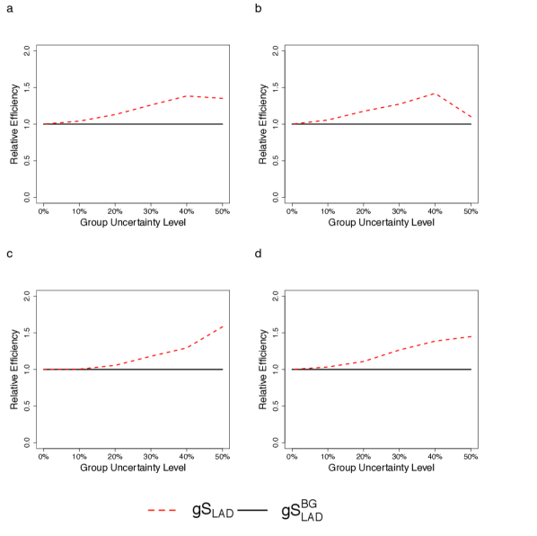
Figure 1: Relative efficiency of $gS_{LAD}^{BG}$ and $gS_{LAD}$ under simulation model 2. $gS_{LAD}^{BG}$ denotes $gS_{LAD}$ applied to the “best-guess” genotype data, and the relative efficiency is the power of $gS_{LAD}$ divided by the power of $gS_{LAD}^{BG}$. The true genotypes were masked using a Dirichlet distribution with scale parameters $a$ for the correct genotype and $(1-a)/2$ for the other two. On average, $a=0.5$ corresponds to 50% group uncertainty, and $a=1$ corresponds to no genotype uncertainty (i.e. 0%). Parameter values included $n/2=500$ sib pairs, and $\rho=0.5$ within-pair correlation. The MAF and $(\sigma_{0}^{2},\sigma_{1}^{2},\sigma_{2}^{2})$ were 0.1 and (1, 1.5, 2) for (a), 0.1 and (2, 1.5, 1) for (b), 0.2 and (1, 1.5, 2) for (c), and 0.2, (2, 1.5, 1) for (d). Power was estimated from 1,000 simulated replicates at the 5% level. The absolute power of $gS_{LAD}^{BG}$ and $gS_{LAD}$ at the 30% group uncertainty level for (a) and (c) are presented in Table A Generalized Levene’s Scale Test for Variance Heterogeneity in the Presence of Sample Correlation and Group Uncertainty under Gaussian data.

References

- Abney (2015) Abney, M. (2015). Permutation testing in the presence of polygenic variation. Genet Epidemiol 39, 249–58.
- Acar and Sun (2013) Acar, E. F. and Sun, L. (2013). A generalized Kruskal-Wallis test incorporating group uncertainty with application to genetic association studies. Biometrics 69, 427–35.
- Aitken (1936) Aitken, A. C. (1936). On least squares and linear combination of observations. Proceedings of the Royal Society of Edinburgh 55, 42–48.
- Arnold (1980) Arnold, S. F. (1980). Asymptotic validity of F tests for the ordinary linear model and the multiple correlation model. Journal of the American Statistical Association 75, 890–894.
- Baltagi (2008) Baltagi, B. H. (2008). Econometrics. Springer-Verlag, Berlin, Heidelberg, fourth edition.
- Bartlett (1937) Bartlett, M. S. (1937). Properties of sufficiency and statistical tests. Proceedings of the Royal Society of London. Series A, Mathematical and Physical Sciences 160, 268–282.
- Breusch and Pagan (1979) Breusch, T. S. and Pagan, A. R. (1979). A simple test for heteroscedasticity and random coefficient variation. Econometrica 47, 1287–1294.
- Brown and Forsythe (1974) Brown, M. B. and Forsythe, A. B. (1974). Robust tests for the equality of variances. Journal of the American Statistical Association 69, 364–367.
- Cameron and Miller (2013) Cameron, A. C. and Miller, D. L. (2013). A practitioner’s guide to cluster-robust inference. Forthcoming in Journal of Human Resources pages 221–236.
- Cao et al. (2014) Cao, Y., Wei, P., Bailey, M., Kauwe, J. S., Maxwell, T. J., and the Alzheimer’s Disease Neuroimaging Initiative (2014). A versatile omnibus test for detecting mean and variance heterogeneity. Genet Epidemiol 38, 51–9.
- Carroll and Schneider (1985) Carroll, R. J. and Schneider, H. (1985). A note on Levene’s tests for equality of variances. Statistics Probability Letters 3, 191–194.
- Conover et al. (1981) Conover, W. J., Johnson, M. E., and Johnson, M. M. (1981). A comparative study of tests for homogeneity of variances, with applications to the outer continental shelf bidding data. Technometrics 23, 351–361.
- Cook and Weisberg (1983) Cook, R. D. and Weisberg, S. (1983). Diagnostics for heteroscedasticity in regression. Biometrika 70, 1–10.
- Derkach et al. (2013) Derkach, A., Lawless, J. F., and Sun, L. (2013). Robust and powerful tests for rare variants using Fisher’s method to combine evidence of association from two or more complementary tests. Genet Epidemiol 37, 110–21.
- Derkach et al. (2014) Derkach, A., Lawless, J. F., and Sun, L. (2014). Pooled association tests for rare genetic variants: A review and some new results. Statistical Science 29, 302–321.
- Furno (2005) Furno, M. (2005). The Glejser test and the median regression. Sankhyā: The Indian Journal of Statistics pages 335–358.
- Gastwirth et al. (2009) Gastwirth, J. L., Gel, Y. R., and Miao, W. (2009). The impact of Levene’s test of equality of variances on statistical theory and practice. Statistical Science pages 343–360.
- Glejser (1969) Glejser, H. (1969). A new test for heteroskedasticity. Journal of the American Statistical Association 64, 316–323.
- Godfrey (1996) Godfrey, L. G. (1996). Some results on the Glejser and Koenker tests for heteroskedasticity. Journal of Econometrics 72, 275–299.
- Haseman and Elston (1970) Haseman, J. K. and Elston, R. C. (1970). The estimation of genetic variance from twin data. Behav Genet 1, 11–9.
- Horvath et al. (2001) Horvath, S., Xu, X., and Laird, N. M. (2001). The family based association test method: strategies for studying general genotype–phenotype associations. Eur J Hum Genet 9, 301–6.
- Iachine et al. (2010) Iachine, I., Petersen, H. C., and Kyvik, K. O. (2010). Robust tests for the equality of variances for clustered data. Journal of Statistical Computation and Simulation 80, 365–377.
- Im (2000) Im, K. S. (2000). Robustifying Glejser test of heteroskedasticity. Journal of Econometrics 97, 179–188.
- Jakobsdottir and McPeek (2013) Jakobsdottir, J. and McPeek, M. S. (2013). MASTOR: mixed-model association mapping of quantitative traits in samples with related individuals. Am J Hum Genet 92, 652–66.
- Keyes and Levy (1997) Keyes, T. K. and Levy, M. S. (1997). Analysis of Levene’s test under design imbalance. Journal of Educational and Behavioral Statistics 22, 227–236.
- Kutalik et al. (2011) Kutalik, Z., Johnson, T., Bochud, M., Mooser, V., Vollenweider, P., Waeber, G., and et al. (2011). Methods for testing association between uncertain genotypes and quantitative traits. Biostatistics 12, 1–17.
- Levene (1960) Levene, H. (1960). Robust tests for equality of variances. In Olkin, I., editor, Contributions to probability and statistics; essays in honor of Harold Hotelling, pages 278–292. Stanford University Press, Stanford, Calif.
- Li et al. (2014) Li, W., Soave, D., Miller, M. R., Keenan, K., Lin, F., Gong, J., and et al. (2014). Unraveling the complex genetic model for cystic fibrosis: pleiotropic effects of modifier genes on early cystic fibrosis-related morbidities. Hum Genet 133, 151–61.
- Lim and Loh (1996) Lim, T.-S. and Loh, W.-Y. (1996). A comparison of tests of equality of variances. Computational Statistics Data Analysis 22, 287–301.
- Machado and Silva (2000) Machado, J. A. F. and Silva, J. M. C. S. (2000). Glejser’s test revisited. Journal of Econometrics 97, 189–202.
- Marozzi (2013) Marozzi, M. (2013). Nonparametric simultaneous tests for location and scale testing: A comparison of several methods. Communications in Statistics - Simulation and Computation 42, 1298–1317.
- O’Neill and Mathews (2000) O’Neill, M. E. and Mathews, K. (2000). Theory methods: A weighted least squares approach to Levene’s test of homogeneity of variance. Australian New Zealand Journal of Statistics 42, 81–100.
- Owen (2009) Owen, A. B. (2009). Karl Pearson’s meta-analysis revisited. Ann Statist pages 3867–3892.
- Pare et al. (2010) Pare, G., Cook, N. R., Ridker, P. M., and Chasman, D. I. (2010). On the use of variance per genotype as a tool to identify quantitative trait interaction effects: a report from the women’s genome health study. PLoS Genet 6, e1000981.
- Paterson et al. (2010) Paterson, A. D., Waggott, D., Boright, A. P., Hosseini, S. M., Shen, E., Sylvestre, M. P., and et al. (2010). A genome-wide association study identifies a novel major locus for glycemic control in type 1 diabetes, as measured by both A1C and glucose. Diabetes 59, 539–49.
- Pinheiro and Bates (2000) Pinheiro, J. C. and Bates, D. M. (2000). Mixed-effects models in S and S-PLUS. Statistics and computing. Springer, New York.
- Soave et al. (2015) Soave, D., Corvol, H., Panjwani, N., Gong, J., Li, W., Boelle, P. Y., and et al. (2015). A joint location-scale test improves power to detect associated SNPs, gene sets, and pathways. Am J Hum Genet 97, 125–38.
- Sun (2012) Sun, L. (2012). Detecting pedigree relationship errors. In Elston, C. R., Satagopan, M. J., and Sun, S., editors, Statistical Human Genetics: Methods and Protocols, pages 25–46. Humana Press, Totowa, NJ.
- Sun and Dimitromanolakis (2012) Sun, L. and Dimitromanolakis, A. (2012). Identifying cryptic relationships. In Elston, C. R., Satagopan, M. J., and Sun, S., editors, Statistical Human Genetics: Methods and Protocols, pages 47–57. Humana Press, Totowa, NJ.
- Sun et al. (2012) Sun, L., Rommens, J. M., Corvol, H., Li, W., Li, X., Chiang, T. A., and et al. (2012). Multiple apical plasma membrane constituents are associated with susceptibility to meconium ileus in individuals with cystic fibrosis. Nat Genet 44, 562–9.
- Sun et al. (2013) Sun, X., Elston, R., Morris, N., and Zhu, X. (2013). What is the significance of difference in phenotypic variability across snp genotypes? Am J Hum Genet 93, 390–7.
- Taylor et al. (2011) Taylor, C., Commander, C. W., Collaco, J. M., Strug, L. J., Li, W., Wright, F. A., and et al. (2011). A novel lung disease phenotype adjusted for mortality attrition for cystic fibrosis genetic modifier studies. Pediatr Pulmonol 46, 857–69.
- Thompson (1975) Thompson, E. A. (1975). The estimation of pairwise relationships. Ann Hum Genet 39, 173–88.
- Visscher and Posthuma (2010) Visscher, P. M. and Posthuma, D. (2010). Statistical power to detect genetic loci affecting environmental sensitivity. Behav Genet 40, 728–33.
- White (1980) White, H. (1980). A heteroskedasticity-consistent covariance matrix estimator and a direct test for heteroskedasticity. Econometrica 48, 817–838.
- Yang et al. (2011) Yang, Y., Christensen, O. F., and Sorensen, D. (2011). Use of genomic models to study genetic control of environmental variance. Genet Res (Camb) 93, 125–38.