A Framework for FFT-based Homogenization on Anisotropic Lattices

Abstract

Abstract. In order to take structural anisotropies of a given composite and different shapes of its unit cell into account, we generalize the Basic Scheme in homogenization by Moulinec and Suquet to arbitrary sampling lattices and tilings of the $d$-dimensional Euclidean space. We employ a Fourier transform for these lattices by introducing the corresponding set of sample points, the so called pattern, and its frequency set, the generating set, both representing the anisotropy of both the shape of the unit cell and the chosen preferences in certain sampling directions. In several cases, this Fourier transform is of lower dimension than the space itself. For the so called rank-$1$-lattices it even reduces to a one-dimensional Fourier transform having the same leading coefficient as the fastest Fourier transform implementation available. We illustrate the generalized Basic Scheme on an anisotropic laminate and a generalized ellipsoidal Hashin structure. For both we give an analytical solution to the elasticity problem, in two- and three dimensions, respectively. We then illustrate the possibilities of choosing a pattern. Compared to classical grids this introduces both a reduction of computation time and a reduced error of the numerical method. It also allows for anisotropic subsampling, i.e. choosing a sub lattice of a pixel or voxel grid based on anisotropy information of the material at hand.
Key words. elasticity, homogenization, Fourier transform, lattices, Lippmann-Schwinger equation
AMS classification. 42B37, 42B05, 65T50, 74B05, 74E30

1 Introduction

Modern materials are often composites of multiple components which are designed to obtain overall properties like high durability, flexibility or stiffness. These inhomogeneities are usually small in comparison to the overall structure of the material or tool. Therefore it is computationally beneficial and sometimes even necessary to replace the inhomogeneous material by a homogeneous one having the same macroscopic properties, called homogenization.

The underlying assumption is that the microstructure can be represented by a reference volume that can be repeated periodically to generate the geometry. While many of these microstructures show macroscopically isotropic behavior there are also composites that have one or multiple predominant directions.

The classical algorithm to solve such homogenization problems of periodic microstructures on regular grids was proposed by Moulinec and Suquet [20, 21]. This algorithm is also called the Basic Scheme and has evoked many enhancements and modifications. Amongst them are different discretization methods of the differential operator [30, 25, 24], adaptions to composites with infinite contrast, e.g. porous media, [18, 24], incorporation of additional information about the geometry [12] and the solution of homogenization problems of higher order [27].

All of them have in common that they are formulated on regular tensor product grids, i.e. they make use of the commonly known multidimensional Fast Fourier Transform (FFT). In some cases it is not possible to rotate the representative volume element without violating the periodicity condition of the microstructure and then a change of the discretization grid can remedy this.

Galipeau and Castañeda [10, 9], for example, construct a periodic laminate structure of elastomers where each of the two phases consists of aligned elongated particles of a magnetic material. In this material, the two phases differ in orientation and do not face into the direction of lamination nor orthogonal to it. Lahellec, et. al. [15] consider a multi-particle problem where they have an evolving computational grid. The basis vectors of this grid depend on the macroscopic velocity of a Newtonian fluid and they hint that the grid for the FFT does not have to be a rectangular one without elaborating this point. In both cases it might be beneficial to consider a more general sampling, i.e. sampling on anisotropic lattices.

Besides the theory of a discrete Fourier transform (DFT) on abelian groups, also known as generalized Fourier transform [1], the DFT has also been generalized to arbitrary sampling lattices, e.g. in order to derive periodic wavelets [16, 6] and a corresponding fast Fourier and fast wavelet transform [2]. The computational complexity on these lattices even stays the same as on the usual rectangular or pixel grid.

Furthermore using the theory of rank-1-lattices, Kämmerer et al. [14, 13] and Potts and Volkmer [22] derive several adaptive schemes to approximate both a certain set of frequencies as well as a set of sampling points and derive approximation errors for functions of certain smoothness. This also includes a constructive derivation of the vector that generates the lattice. For these special lattices, the Fourier transform even in high-dimensional space reduces to a one-dimensional Fourier transform and hence reducing both the organization of the sampled data and the computational cost to compute the FFT. The theory of rank-1-lattices therefore both allows for directly taking known anisotropic properties of a function into account and thereby reducing the necessary number of sample values or measurements by adapting the lattice. Furthermore it also reduces the computational cost or data organization overhead due to the reduction from a high-dimensional FFT to a one-dimensional one.

In this paper we generalize the Basic Scheme by Moulinec and Suquet to arbitrary anisotropic periodic lattices. This introduces the possibility to prefer directions other than the coordinate axes in the reference volume and hence in the solution. This allows for aligning the basis functions with the dominant orientations of the geometry and controlling the refinement in these directions. This generalization of the Basic Scheme to arbitrary anisotropic sampling lattices introduces the form of the grid as a algorithmic parameter without additional computational costs. For a special set of rank-1-lattices, after sampling in a high-dimensional space, the computation of the fast Fourier transform even reduces to a one-dimensional FFT. Therefore, additionally to the new possibility of choosing directions of preference, one can also choose these to reduce the computational efforts.

The remainder of the paper is organized as follows. In Section 2 we establish the preliminaries regarding the parametrization, properties of anisotropic lattices and their patterns on the unit cube. Further, we introduce the FFT on such patterns, where the usual tensor product grid is a special case. Exemplary for a homogenization problem we introduce the periodic equations of quasi-static elasticity in Section 3 and elaborate on the unmodified Basic Scheme how to generalize it. Based on this we explain the difference between making a coordinate transformation and choosing a lattice adapted to the geometry of the lattice. In Section 4 we generalize two known geometries to an anisotropic setting: the laminate structure and the Hashin structure that serves as the main analytical example for this work. Both are anisotropic structures within isotropic material laws that provide an analytic solution for the strain field and the effective matrix. This allows us to study effect of the pattern orientation on the solution and the effective properties in Section 5.

2 Preliminaries

Throughout this paper we will employ the following notation: The symbols $a\in\mathbb{C}$, $\mathbf{a}\in\mathbb{C}^{d}$ and $\mathbf{A}\in\mathbb{C}^{d\times d}$ denote scalars, vectors, and matrices, respectively. The only exception from this are $f,g,h$ which are reserved for functions. We denote the inner product of two vectors by $\mathbf{a}^{\mathrm{T}}\mathbf{b}\coloneqq\sum_{i}a_{i}b_{i}$ and reserve the symbol $\langle\cdot,\cdot\rangle$ for inner products of two functions or two generalized sequences, respectively. For a complex number $a=b+{\mathrm{i}}c$, $b,c\in\mathbb{R}$, we denote the complex conjugate by $\overline{a}\coloneqq b+{\mathrm{i}}c$.

Usually, we are concerned with $d$-dimensional data, where $d=2,3$, but the theory can also be written in arbitrary dimensions. Sets are denoted by capital case calligraphic letters, e.g. $\mathcal{P}(\cdot)$ or $\mathcal{G}(\cdot)$ and the same for the Fourier transform $\mathcal{F}(\cdot)$; all of these might depend on a scalar $n$ or matrix $\mathbf{M}$ given in brackets. We denote second-order tensors by small Greek letters as $\lambda,\epsilon$ with entries $\lambda_{ij}$ are indexed again by scalars $i,j$ and similarly we denote fourth-order tensors by capital calligraphic letters, where $\mathcal{C}$ is the most prominent one. Finally, constants like Euler’s number ${\,\mathrm{e}}$ or the imaginary unit ${\mathrm{i}}$, i.e. ${\mathrm{i}}^{2}=-1$, are set upright.

2.1 Arbitrary patterns and the Fourier transform

The space of functions we are concerned with is the Hilbert space $L^{2}(\mathbb{T}^{d})$ of (equivalence classes of) square integrable functions on the $d$-dimensional torus $\mathbb{T}\cong[-\pi,\pi)^{d}$ with inner product

$$\langle f,g\rangle=\frac{1}{(2\pi)^{d}}\int_{\mathbb{T}^{d}}f(\mathbf{x})\overline{g(\mathbf{x})}\,\mathrm{d}\mathbf{x},\qquad f,g\in L^{2}(\mathbb{T}^{d})\text{.}$$

In several cases, the functions of interest are tensor-valued. For these functions, we take the tensor product of the Hilbert space, e.g. $L^{2}(\mathbb{T}^{d})^{n\times n}$ for the space of functions $f\colon\mathbb{T}^{d}\to\mathbb{C}^{n\times n}$ that have values being $n\times n$-dimensional matrices. The following Fourier transform can be generalized to these tensor product spaces by performing the operations element wise. We restrict the following preliminaries of this subsection therefore to the case of $L^{2}(\mathbb{T}^{d})$.

Every function $f\in L^{2}(\mathbb{T}^{d})$ can be written in its Fourier series representation

$$f(\mathbf{x})=\sum_{\mathbf{k}\in\mathbb{Z}^{d}}c_{\mathbf{k}}(f){\,\mathrm{e}}^{{\mathrm{i}}\mathbf{k}^{\mathrm{T}}\mathbf{x}},$$ (1)

introducing the the multivariate Fourier coefficients $c_{\mathbf{k}}(f)=\langle f,{\,\mathrm{e}}^{{\mathrm{i}}\mathbf{k}^{\mathrm{T}}\circ}\rangle$, $\mathbf{k}\in\mathbb{Z}^{d}$. The equality in (1) is meant in $L^{2}(\mathbb{T}^{d})$ sense. We denote by $\mathbf{c}(f)=\bigl{\{}(c_{\mathbf{k}}(f)\bigr{\}}_{\mathbf{k}\in\mathbb{Z}^{d}}\in\ell^{2}(\mathbb{Z}^{d})$ the generalized sequences which form a Hilbert space with the inner product

$$\langle\mathbf{c},\mathbf{d}\rangle=\sum_{\mathbf{k}\in\mathbb{Z}^{d}}c_{\mathbf{k}}\overline{d_{\mathbf{k}}},\qquad\mathbf{c},\mathbf{d}\in\ell^{2}(\mathbb{Z}^{d})\text{.}$$

The Parseval equation reads

$$\langle f,g\rangle=\langle\mathbf{c}(f),\mathbf{c}(g)\rangle=\sum_{\mathbf{k}\in\mathbb{Z}^{d}}c_{\mathbf{k}}(f)\overline{c_{\mathbf{k}}(g)}\text{.}$$ (2)

The pattern and the generating set

For any regular matrix $\mathbf{M}\in\mathbb{Z}^{d\times d}$, we define the congruence relation for $\mathbf{h},\mathbf{k}\in\mathbb{Z}^{d}$ with respect to $\mathbf{M}$ by

$$\mathbf{h}\equiv\mathbf{k}\bmod\mathbf{M}\Leftrightarrow\exists\,\mathbf{z}\in\mathbb{Z}^{d}\colon\mathbf{k}=\mathbf{h}+\mathbf{M}\mathbf{z}\text{.}$$

We define the lattice

$$\Lambda(\mathbf{M})\coloneqq\mathbf{M}^{-1}\mathbb{Z}^{d}=\{\mathbf{y}\in\mathbb{R}^{d}:\mathbf{M}\mathbf{y}\in\mathbb{Z}^{d}\},$$

and the pattern $\operatorname{\mathcal{P}}(\mathbf{M})$ as any set of congruence representant of the lattice with respect to $\bmod\ 1$, e.g. $\Lambda(\mathbf{M})\cap[0,1)^{d}$ or $\Lambda(\mathbf{M})\cap\bigl{[}-\tfrac{1}{2},\tfrac{1}{2}\bigr{)}^{d}$. For the rest of the paper we will refer to the set of congruence class representants in the symmetric unit cube $\bigl{[}-\tfrac{1}{2},\tfrac{1}{2}\bigr{)}^{d}$. The generating set $\operatorname{\mathcal{G}}(\mathbf{M})$ is defined by $\operatorname{\mathcal{G}}(\mathbf{M})\coloneqq\mathbf{M}\operatorname{\mathcal{P}}(\mathbf{M})$ for any pattern $\operatorname{\mathcal{P}}(\mathbf{M})$. For both, the number of elements is given by $\lvert\operatorname{\mathcal{P}}(\mathbf{M})\rvert=\lvert\operatorname{\mathcal{G}}(\mathbf{M})\rvert=\lvert\det{\mathbf{M}}\rvert\eqqcolon m,$ which follows directly from [7, Lemma II.7].

Finally for any factorization $\mathbf{M}=\mathbf{J}\mathbf{N}$ of an integer matrix $\mathbf{M}\in\mathbb{Z}^{d\times d}$ into two integer matrices $\mathbf{J},\mathbf{N}\in\mathbb{Z}^{d}$, we have

$$\mathbf{x}\in\Lambda(\mathbf{N})\Rightarrow\mathbf{N}\mathbf{x}\in\mathbb{Z}^{d}\Rightarrow\mathbf{J}\mathbf{N}\mathbf{x}\in\mathbb{Z}^{d},$$

and hence $\Lambda(\mathbf{N})\subset\Lambda(\mathbf{M})$. By construction of the pattern, we directly obtain $\operatorname{\mathcal{P}}(\mathbf{N})\subset\operatorname{\mathcal{P}}(\mathbf{M})$; see [16, Lemma 2.7] and [2, Section 2] for a more general introduction. We call the smaller pattern $\operatorname{\mathcal{P}}(\mathbf{N})$ a subpattern of $\operatorname{\mathcal{P}}(\mathbf{M})$. Note that this is not commutative with respect to $\mathbf{J}$ and $\mathbf{N}$. Looking at the generating sets for the decomposition $\mathbf{M}=\mathbf{JN}$ we have $\operatorname{\mathcal{G}}(\mathbf{N}^{\mathrm{T}})\subset\operatorname{\mathcal{G}}(\mathbf{M}^{\mathrm{T}})$. A subpattern of a tensor product grid, the so called quincunx pattern, is shown in Fig. 1, left.

2.2 A fast Fourier transform on patterns

The discrete Fourier transform on the pattern $\operatorname{\mathcal{P}}(\mathbf{M})$ is defined [8] by

$$\mathcal{F}(\mathbf{M})\coloneqq\frac{1}{m}\Bigl{(}{\,\mathrm{e}}^{-2\pi{\mathrm{i}}\mathbf{h}^{\mathrm{T}}\mathbf{y}}\Bigr{)}_{\mathbf{h}\in\operatorname{\mathcal{G}}(\mathbf{M}^{\mathrm{T}}),\,\mathbf{y}\in\operatorname{\mathcal{P}}(\mathbf{M})},$$ (3)

where $\mathbf{h}\in\operatorname{\mathcal{G}}(\mathbf{M}^{\mathrm{T}})$ indicate the rows and $\mathbf{y}\in\operatorname{\mathcal{P}}(\mathbf{M})$ indicate the columns of the Fourier matrix $\mathcal{F}(\mathbf{M})$. This discrete Fourier transform was also investigated in [2, 16]. For both the pattern $\operatorname{\mathcal{P}}(\mathbf{M})$ and the generating set $\operatorname{\mathcal{G}}(\mathbf{M}^{\mathrm{T}})$, an arbitrary but fixed ordering has to be chosen. The discrete Fourier transform on $\operatorname{\mathcal{P}}(\mathbf{M})$ is defined for a vector $\mathbf{a}=(a_{\mathbf{y}})_{\mathbf{y}\in\operatorname{\mathcal{P}}(\mathbf{M})}\in\mathbb{C}^{m}$ arranged in the same ordering as the columns in (3) by

$$\mathbf{\hat{a}}=(\hat{a}_{\mathbf{h}})_{\mathbf{h}\in\operatorname{\mathcal{G}}(\mathbf{M}^{\mathrm{T}})}=\mathcal{F}(\mathbf{M})\mathbf{a},$$ (4)

where the resulting vector $\mathbf{\hat{a}}$ is ordered as the columns of $\mathcal{F}(\mathbf{M})$ in (3).

For a diagonal matrix $\mathbf{M}=\operatorname{diag}(n,n)\in\mathbb{N}^{2\times 2}$ having the same entry $n\in\mathbb{N}$ on both diagonal entries, the pattern $\operatorname{\mathcal{P}}(\mathbf{M})$ is the set $\bigl{(}y_{1},y_{2})^{\mathrm{T}},y_{1},y_{2}\in\frac{1}{m}\{0,\ldots,m-1\}$. The generating set $\operatorname{\mathcal{G}}(\mathbf{M})$ then reads $\{\mathbf{k}\in\mathbb{Z}^{2}:0\leq k_{j}\leq m-1,j=1,2\}$. Both have $m=n^{2}$ elements. The Fourier transform for this diagonal matrix is just the usual 2D DFT.

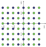
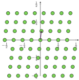
Figure 1: By choosing $\mathbf{M}_{1}=\mathbf{JN}=\bigl{(}\begin{smallmatrix}1&-1\\ 1&1\end{smallmatrix}\bigr{)}\bigl{(}\begin{smallmatrix}4&4\\ -4&4\end{smallmatrix}\bigr{)}$ we obtain a usual rectangular grid pattern $\operatorname{\mathcal{P}}(\mathbf{M}_{1})$ (left) of a diagonal matrix and its sub pattern $\operatorname{\mathcal{P}}(\mathbf{N}$ (dark), a quincux pattern. We can prefer certain directions like for pattern $\operatorname{\mathcal{P}}(\mathbf{M}_{2})$, $\mathbf{M}_{2}=\bigl{(}\begin{smallmatrix}8&-4\\ 2&7\end{smallmatrix}\bigr{)}$, (middle). Certain patterns, like $\operatorname{\mathcal{P}}(\mathbf{M}_{3})$, $\mathbf{M}_{3}=\bigl{(}\begin{smallmatrix}8&-1\\ 0&8\end{smallmatrix}\bigr{)}$, (right) are even generated by only one generating vector. Note that all matrices have the same determinant and hence the patterns have the same number of points.

Fig. 1 illustrates that the Fourier transform (4) generalizes the usual discretization on a pixel grid and enables to prefer certain directions by choosing different patterns having the same number of points.

To efficiently implement the Fourier transform (4) on an arbitrary pattern $\operatorname{\mathcal{P}}(\mathbf{M)}$ for a regular integer matrix $\mathbf{M}\in\mathbb{Z}^{d\times d}$, we have to fix a certain order of the elements therein. Following the construction in [2], we use the Smith normal form $\mathbf{M}=\mathbf{QER}$, where $\mathbf{Q},\mathbf{R}$ are of determinant $1$ and $\mathbf{E}=\operatorname{diag}(e_{1},\ldots,e_{d})$ is the diagonal matrix of elementary divisors where $e_{j}$ is a divisor of $e_{j+1}$, $j=1,\ldots,d-1$. We further denote by $d_{\mathbf{M}}\coloneqq\lvert\{j:e_{j}>1\}\rvert$ the dimension of the pattern. For the special case, that $d_{\mathbf{M}}=1$, the lattice is also called rank-$1$-lattice. Such a lattice is shown in Fig. 1 (right)

Introducing the pattern basis vector(s)

$$\mathbf{y}_{j}\coloneqq\frac{1}{e_{d+d_{\mathbf{M}}+j}}\mathbf{e}_{d-d_{\mathbf{M}}+j},\qquad j=1,\ldots,d_{\mathbf{M}},$$ (5)

where $\mathbf{e}_{j}$ denotes the $j$th unit vector, we obtain a basis for the pattern. Hence we can write

$$\mathbf{y}=\sum_{j=1}^{d_{\mathbf{M}}}\lambda_{j}\mathbf{y}_{j},\qquad\lambda_{j}\in\{0,\ldots,e_{j}-1\},\ j=1,\ldots,d_{\mathbf{M}},$$

where the summation is meant on the congruence classes, i.e. with respect to $\bmod\ 1$ onto the pattern $\operatorname{\mathcal{P}}(\mathbf{M})$, we obtain a unique addressing for each pattern point using the coefficients $\lambda_{1},\ldots,\lambda_{d_{\mathbf{M}}}$. With the lexicographical ordering of the vectors $(0,\ldots,0)^{\mathrm{T}},\ldots,$
$(\lambda_{1}-1,\ldots,\lambda_{d_{\mathbf{M}}}-1)$ one not only obtains an array representation of any coefficient vector

$$\mathbf{a}=\bigl{(}a_{\mathbf{y}}\bigr{)}_{\mathbf{y}\in\operatorname{\mathcal{P}}(\mathbf{M})}=\bigl{(}a_{\lambda_{1},\ldots,\lambda_{d_{\mathbf{M}}}}\bigr{)}_{\lambda_{1}=0,\ldots,\lambda_{d_{\mathbf{M}}}=0}^{e_{d-d_{\mathbf{M}}+1}-1,\ldots,e_{d}-1},$$

but similarly also for any vector $\hat{\mathbf{a}}$ corresponding to the generating set using the generating set basis vector(s)

$$\mathbf{h}_{j}\coloneqq\mathbf{M}^{\mathrm{T}}\tilde{\mathbf{y}}_{j}=\mathbf{R}^{\mathrm{T}}\mathbf{e}_{j},\qquad j=1,\ldots,d_{\mathbf{M}},$$ (6)

where $\tilde{\mathbf{y}}$ denotes the basis vector(s) of $\operatorname{\mathcal{P}}(\mathbf{M}^{\mathrm{T}})$ constructed as above. Note that the pattern dimension $d_{\mathbf{M}}=d_{\mathbf{M}^{\mathrm{T}}}$ and the elementary divisors $e_{j}$ are identical for the patterns $\operatorname{\mathcal{P}}(\mathbf{M})$ and $\operatorname{\mathcal{P}}(\mathbf{M}^{\mathrm{T}})$.

With these fixed orderings of the vector entries of $\mathbf{a}$ and $\hat{\mathbf{a}}$, the Fourier transform (4) can be computed using an ordinary $d_{\mathbf{M}}$-dimensional Fourier transform even having the same leading coefficient in its complexity of $\mathcal{O}(m\log m)$ [2, Theorem 2]. Note that for rank-1-lattices, the Fourier transform on the pattern even reduces to a one-dimensional FFT for patterns in 2, 3 or even more dimensions.

Sampling and aliasing

Let $f\in L_{2}(\mathbb{T}^{d})$ denote a square integrable function on the torus, such that its Fourier series (1) converges absolutely, i.e.

$$\sum_{\mathbf{k}\in\mathbb{Z}^{d}}\lvert c_{\mathbf{k}}((f))\rvert<\infty.$$

Sampling $f$ at the points given by pattern $\operatorname{\mathcal{P}}(\mathbf{M})$ of a regular matrix $\mathbf{M}\in\mathbb{Z}^{d\times d}$, i.e. $a_{\mathbf{y}}\coloneqq f(2\pi\mathbf{y})$, $\mathbf{y}\in\operatorname{\mathcal{P}}(\mathbf{M})$, and performing a discrete Fourier transform we obtain the discrete Fourier coefficients $c_{\mathbf{h}}^{\mathbf{M}}(f)=\hat{a}_{\mathbf{h}}$, $\mathbf{h}\in\operatorname{\mathcal{G}}(\mathbf{M}^{\mathrm{T}})$, where $\mathbf{\hat{a}}=\mathcal{F}(\mathbf{M})\mathbf{a}$. A relation between the Fourier coefficients $c_{\mathbf{k}}(f)$ and the discrete Fourier coefficients $c_{\mathbf{h}}^{\mathbf{M}}(f)$ is given by the following Lemma.

Lemma 2.1.

Let $f\in L^{2}(\mathbb{T}^{d})$ with absolutely convergent Fourier series and the regular matrix $\mathbf{M}\in\mathbb{Z}^{d\times d}$ be given. Then the discrete Fourier coefficients $c_{\mathbf{h}}^{\mathbf{M}}(f)$, $\mathbf{h}\in\operatorname{\mathcal{G}}(\mathbf{M}^{\mathrm{T}})$, fulfill the relation

$$c_{\mathbf{h}}^{\mathbf{M}}(f)=\sum_{\mathbf{z}\in\mathbb{Z}^{d}}c_{\mathbf{h}+\mathbf{M}^{\mathrm{T}}\mathbf{z}}(f),\qquad\mathbf{h}\in\operatorname{\mathcal{G}}(\mathbf{M)^{\mathrm{T}}}\text{.}$$ (7)

For a proof, see [5, Lemma 2]. This Lemma is also called Aliasing formula and can be interpreted as follows: If the Fourier coefficients $c_{\mathbf{k}}(f)$ of $f$ decay slowly along a certain direction $\mathbf{h}_{j}$ being a basis vector of $\operatorname{\mathcal{G}}(\mathbf{M}^{\mathrm{T}}$) and the corresponding $\epsilon_{j}$ is small, then the effect of the summands $\mathbf{z}\neq\mathbf{0}$ is quite large or in other words the approximation $c_{\mathbf{h}}^{\mathbf{M}}(f)\approx c_{\mathbf{h}}(f)$ is not sufficient enough. This might be e.g. due to presence of an edge orthogonal to $\mathbf{h}_{j}$. If on the other hand, the spectrum is bounded in this direction and $\epsilon_{j}$ is large enough, then the approximation is of better quality.

Pattern congruence classes

Following the pattern classification, cf. [16, Section 2.4] we notice that $\operatorname{\mathcal{P}}(\mathbf{M})=\operatorname{\mathcal{P}}(\mathbf{N})$ whenever $\mathbf{M}=\mathbf{Q}\mathbf{N}$ holds for a matrix $\mathbf{Q}\in\mathbb{Z}^{d\times d}$, $\lvert\det\mathbf{Q}\rvert=1$. We define the pattern congruence of two matrices by $\mathbf{M}\sim_{\operatorname{\mathcal{P}}}\mathbf{N}$ whenever they generate the same pattern. By [16, Lemma 2.5] there exists a congruence class representant $\mathbf{M}^{\circ}=(m^{\circ}_{i,j})_{j,i=1}^{d,d}$ in every congruence class, such that $\mathbf{M}^{\circ}$ is upper triangular, and $0\leq m^{\circ}_{i,j}<m^{\circ}_{j,j}$ for all $i<j$.

An easy consequence of this is, that for a diagonal matrix $\mathbf{M}=\bigl{(}\begin{smallmatrix}m_{1}&0\\ 0&m_{2}\end{smallmatrix}\bigr{)}$ choosing $\mathbf{Q}=\bigl{(}\begin{smallmatrix}1&n\\ 0&1\end{smallmatrix})$, $n\in\mathbb{N}$, reveals, that all matrices $\mathbf{M}_{n}\coloneqq\mathbf{Q}\mathbf{M}=\bigl{(}\begin{smallmatrix}m_{1}&m_{2}n\\ 0&m_{2}\end{smallmatrix}\bigr{)}$ possess the same pattern or in other words the same sampling points on the torus. However, their corresponding generating sets $\operatorname{\mathcal{G}}(\mathbf{M}_{n}^{\mathrm{T}})$ differ. This can be interpreted as choosing different directional sine and cosine functions that can be defined on the same set of points in order to analyze given discrete data or employing the periodicity of $c_{\mathbf{h}}^{\mathbf{M}}(f)$ with respect to $\mathbf{M}^{\mathrm{T}}$ that is implied by (7). This introduces the possibility of anisotropic analysis and interpretation even on a usual pixel grid.

From the computational point, two different matrices $\mathbf{M}_{1}\sim_{\operatorname{\mathcal{P}}}\mathbf{M}_{2}$ having the same pattern $\operatorname{\mathcal{P}}(\mathbf{M}_{1})=\operatorname{\mathcal{P}}(\mathbf{M}_{2})$ only require an rearranging of the data arrays due to the change of the basis vectors, i.e. using $\mathbf{y}^{(1)}_{j}$ or $\mathbf{y}^{(2)}_{j}$, $j=1,\ldots,d_{\mathbf{M}_{1}}=d_{\mathbf{M}_{2}}$, when addressing $\mathbf{a}$ in (4) and similarly the ordering with respect to the generating sets $\operatorname{\mathcal{G}}(\mathbf{M}^{\mathrm{T}}_{i})$, $i=1,2$. This rearrangement can easily be computed, see [2, Section 5.2].

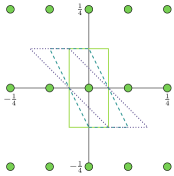
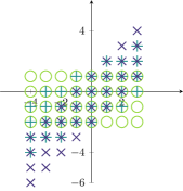
Figure 2: The three matrices $\mathbf{M}=\bigl{(}\begin{smallmatrix}8&4n\\ 0&4\end{smallmatrix}\bigr{)},n=0,1,2$ induce the same sample point set but different scaled unit cells $\frac{1}{2}\mathbf{M}_{n}^{-1}[-1,1]^{2}$ (solid, dashed, dotted; left) and different generating sets $\operatorname{\mathcal{G}}(\mathbf{M}_{n}^{\mathrm{T}})$ ($\circ$, $+$, $\times$; right, respectively) yielding different frequency sets for the Fourier transform.

Example 2.2.

For the simple matrix $\mathbf{M}=\mathbf{M}_{0}=\bigl{(}\begin{smallmatrix}8&0\\ 0&4\end{smallmatrix}\bigr{)}$ the pattern is just the rectangular sampling grid, a subset of which is displayed in Fig. 2 (left). The two matrices $\mathbf{M}_{1}=\bigl{(}\begin{smallmatrix}8&4\\ 0&4\end{smallmatrix}\bigr{)}$ and $\mathbf{M}_{2}=\bigl{(}\begin{smallmatrix}8&8\\ 0&4\end{smallmatrix}\bigr{)}$ possess the same sample points. However, their scaled unit cells $\frac{1}{2}\mathbf{M}_{i}^{-1}[-1,1]^{2}$, also shown in Fig. 2 (left), differ. This illustrates the different directional preference of these matrices, though they possess the same sampling lattice. While the diagonal matrix resembles the form of (stretched) pixels, the shear introduced by looking at other sine/cosine terms can be clearly seen for $i=1,2$ for the dashed and dotted parallelotopes. The three different generating sets $\operatorname{\mathcal{G}}(\mathbf{M}_{n}^{\mathrm{T}})$, $n=1,2,3$ are denoted as circles, pluses and crosses in Fig. 2(right), respectively. Hence both figures illustrate one way to visualize the anisotropy.

3 Homogenization

We want to investigate composite structures which consist of a finite number of materials composed into one material. Common examples are fiber reinforced polymers [12], polycrystalline structures [26] or metall foams [17]. As these structures are typically small they can seldom be resolved exactly in simulations of larger structures. This gives rise to the concept of homogenization where the composite material is replaced by a homogeneous one having the same relevant, i.e. macroscopic, properties. The basic assumption to do this is that the microstructure is periodic, i.e. it is sufficient to look at a representative volume element (RVE) and that the scales of the microstructure and macroscopic structure are separated.

These assumptions allow to calculate the homogenized behavior of the material, the so called effective properties or effective matrix. This can be inserted into a macroscopic calculation or can be used to determine the isotropy of the structure or relevant elastic properties. Typical examples of such problems involve the steady-state heat equation or the quasi-static equation of linear elasticity which we want to focus on henceforth.

3.1 The equation of quasi-static linear elasticity in homogenization

The partial differential equation (PDE) we consider as an example in this publication is the equation of quasi-static linear elasticity. It will serve as the basis to develop a numerical algorithm solving the PDE later on.

Consider a periodic stiffness distribution $\mathcal{C}\in L^{\infty}(\mathbb{T}^{d})^{d\times d\times d\times d}$ that is essentially bounded with major and minor symmetries, i.e. with $\mathcal{C}_{ijkl}=\mathcal{C}_{jikl}=\mathcal{C}_{ijlk}=\mathcal{C}_{klij}$ characterizing the microstructure in the representative volume element. The entries in $\mathcal{C}$ specify the material behavior, e.g. for an isotropic material we have $\mathcal{C}_{ijkl}=\lambda\delta_{ij}\delta_{kl}+\mu(\delta_{ik}\delta_{jl}+\delta_{il}\delta_{jk})$ where $\lambda\in\mathbb{R}$ and $\mu\geq 0$ are the first and second Lamé parameter, respectively.

For the variational formulation of the steady-state heat equation Vordřejc et.al. [29] derive an equivalent integral formula. This approach can be directly applied to the quasi-static linear elasticity equation as follows. We define the space

$$\mathcal{E}(\mathbb{T}^{d})\coloneqq\Bigl{\{}\mathbf{v}\in L^{2}(\mathbb{T}^{d})^{d\times d}:\mathbf{v}=\operatorname{\operatorname{\nabla}_{\mathrm{Sym}}}\mathbf{u},\mathbf{u}\in H^{1}(\mathbb{T}^{d})^{d}\Bigr{\}}$$

where $\operatorname{\operatorname{\nabla}_{\mathrm{Sym}}}\mathbf{u}\coloneqq\frac{1}{2}(\operatorname{\nabla}\mathbf{u}+(\operatorname{\nabla}\mathbf{u})^{\mathrm{T}})$ is the symmetric gradient operator applied to displacement $\mathbf{u}$ and $H^{1}(\mathbb{T}^{d})$ is the Sobolev space with Sobolev index 1, i.e. the space of functions from $L^{2}(\mathbb{T}^{d})$ where the first weak derivative is also in $L^{2}(\mathbb{T}^{d})$.

In the following we will use Einstein’s summation convention. For the product between a symmetric tensor $\mathcal{A}\in\mathbb{R}^{d\times d\times d\times d}$ of fourth order and a symmetric second-order tensor $\alpha\in\mathbb{R}^{d\times d}$ we introduce the notation

$$\mathcal{A}:\alpha\coloneqq(\mathcal{A}_{ijkl}\alpha_{kl})_{ij}.$$

Definition 3.1.

The partial differential equation of quasi-static linear elasticity in homogenization reads:

Find for a macroscopic strain $\epsilon^{0}\in\mathbb{R}^{d\times d}$ the strain function $\tilde{\epsilon}=\tilde{\epsilon}_{\epsilon^{0}}\in\mathcal{E}(\mathbb{T}^{d})$ such that for all $\nu\in\mathcal{E}(\mathbb{T}^{d})$

$$\langle\nu,\mathcal{C}:(\epsilon^{0}+\tilde{\epsilon})\rangle=0$$ (8)

holds true.

We further call $\mathcal{C}^{\mathrm{eff}}\in\mathbb{R}^{d\times d\times d\times d}$ the effective matrix which is connected with the PDE above by

$$\mathcal{C}^{\mathrm{eff}}:\epsilon^{0}\coloneqq\int_{\mathbb{T}^{d}}\mathcal{C}:\bigl{(}\tilde{\epsilon}+\epsilon^{0}\bigr{)}\,\mathrm{d}\mathbf{x}.$$ (9)

By [29] this is equivalent to solving an integral equation for the strain $\epsilon=\tilde{\epsilon}+\epsilon^{0}$ introducing a constant non-zero reference stiffness $\mathcal{C}^{0}$.

Definition 3.2.

The Lippmann-Schwinger equation is given as:

Find $\epsilon\in L^{2}(\mathbb{T}^{d})^{d\times d}$ such that

$$\epsilon=\epsilon^{0}-\operatorname{\operatorname{\nabla}_{\mathrm{Sym}}}(\operatorname{div}:\mathcal{C}^{0}:\operatorname{\operatorname{\nabla}_{\mathrm{Sym}}})^{-1}\operatorname{div}(\mathcal{C}-\mathcal{C}^{0}):\epsilon$$ (10)

in weak sense.

The divergence operator is formally the negative adjoint of the symmetric gradient operator, i.e. $\operatorname{div}=-\operatorname{\operatorname{\nabla}_{\mathrm{Sym}}}^{\mathrm{H}}$, and therefore (10) reduces to finding a strain $\epsilon\in L^{2}(\mathbb{T}^{d})^{d\times d}$ such that

$$\epsilon=\epsilon^{0}-\operatorname{\operatorname{\nabla}_{\mathrm{Sym}}}(\operatorname{\operatorname{\nabla}_{\mathrm{Sym}}}^{\mathrm{H}}:\mathcal{C}^{0}:\operatorname{\operatorname{\nabla}_{\mathrm{Sym}}})^{-1}\operatorname{\operatorname{\nabla}_{\mathrm{Sym}}}^{\mathrm{H}}(\mathcal{C}-\mathcal{C}^{0}):\epsilon,$$ (11)

see [24]. The strain $\epsilon\in L^{2}(\mathbb{T}^{d})^{d\times d}$ can be represented by its Fourier series and we obtain for $\mathbf{k}\in\mathbb{Z}^{d}\setminus\{\mathbf{0}\}$ that

$$c_{\mathbf{k}}(\epsilon)=-\operatorname{\operatorname{\nabla}_{\mathrm{Sym}}}_{\mathbf{k}}(\operatorname{\operatorname{\nabla}_{\mathrm{Sym}}}^{\mathrm{H}}_{\mathbf{k}}:\mathcal{C}^{0}:\operatorname{\operatorname{\nabla}_{\mathrm{Sym}}}_{\mathbf{k}})^{-1}\operatorname{\operatorname{\nabla}_{\mathrm{Sym}}}^{\mathrm{H}}_{\mathbf{k}}c_{\mathbf{k}}\bigl{(}(\mathcal{C}-\mathcal{C}^{0}):\epsilon\bigr{)},$$ (12)

and $c_{\mathbf{0}}(\epsilon)=\epsilon^{0}$. The Fourier multiplier $\operatorname{\operatorname{\nabla}_{\mathrm{Sym}}}_{\mathbf{k}}$ hereby represents the action of the operator $\operatorname{\operatorname{\nabla}_{\mathrm{Sym}}}$ with respect to a Fourier coefficient index $\mathbf{k}\in\mathbb{Z}^{d}\backslash\{\mathbf{0}\}$, respectively. For $u\in H^{1}(\mathbb{T}^{d})^{d}$ it can be derived as

$$c_{\mathbf{k}}(\operatorname{\operatorname{\nabla}_{\mathrm{Sym}}}\mathbf{u})\coloneqq\operatorname{\operatorname{\nabla}_{\mathrm{Sym}}}_{\mathbf{k}}c_{\mathbf{k}}(\mathbf{u})=\frac{{\mathrm{i}}}{2}(\mathbf{k}c_{\mathbf{k}}(\mathbf{u})^{\mathrm{T}}+c_{\mathbf{k}}(\mathbf{u})\mathbf{k}^{\mathrm{T}}).$$ (13)

3.2 Homogenization on anisotropic lattices

The approach of Moulinec and Suquet [20, 21] to discretize (12) is based on collocation on a Cartesian grid, see also [31]. To take into account preferred directions in composite we generalize this approach to arbitrary patterns $\operatorname{\mathcal{P}}(\mathbf{M})$ introduced in the Section 2.

Let a regular integer matrix $\mathbf{M}\in\mathbb{Z}^{d\times d}$ be given. Following the idea of Moulinec and Suquet we collocate (11) at the points $2\pi\mathbf{y}\in\mathbb{T}^{d},\mathbf{y}\in\operatorname{\mathcal{P}}(\mathbf{M})$, of the pattern. This discretization leads to the problem of finding symmetric matrices $\epsilon_{\mathbf{y}}\in\mathbb{R}^{d\times d}$ for each $\mathbf{y}\in\operatorname{\mathcal{P}}(\mathbf{M})$ such that for $\mathbf{y}\in\operatorname{\mathcal{P}}(\mathbf{M})\setminus\{\mathbf{0}\}$ we have

$$\begin{split}\epsilon_{\mathbf{y}}=-&\sum_{\mathbf{h}\in\operatorname{\mathcal{G}}(\mathbf{M}^{\mathrm{T}})}\operatorname{\operatorname{\nabla}_{\mathrm{Sym}}}_{\mathbf{h}}\bigl{(}\operatorname{\operatorname{\nabla}_{\mathrm{Sym}}}^{\mathrm{H}}_{\mathbf{h}}:\mathcal{C}^{0}:\operatorname{\operatorname{\nabla}_{\mathrm{Sym}}}_{\mathbf{h}}\bigr{)}^{-1}\operatorname{\operatorname{\nabla}_{\mathrm{Sym}}}_{\mathbf{h}}\\ &\quad\times\frac{1}{m}\sum_{\mathbf{z}\in\operatorname{\mathcal{P}}(\mathbf{M})}(\mathcal{C}_{\mathbf{z}}-\mathcal{C}^{0}):\epsilon_{\mathbf{z}}{\,\mathrm{e}}^{-2\pi{\mathrm{i}}\mathbf{h}^{\mathrm{T}}\mathbf{z}}{\,\mathrm{e}}^{2\pi{\mathrm{i}}\mathbf{h}^{\mathrm{T}}\mathbf{y}}\end{split}$$ (14)

and $\epsilon_{\mathbf{0}}=\epsilon^{0}$. This discretization gives rise to the generalized basic scheme for patterns based on [21] summarized in Algorithm 1.

$\epsilon^{(0)}_{\mathbf{y}}\leftarrow\epsilon^{0}$ for all $\mathbf{y}\in\operatorname{\mathcal{P}}(\mathbf{M})$

$n\leftarrow 0$

repeat

     $\tau^{(n+1)}_{\mathbf{y}}\leftarrow\left(\mathcal{C}_{\mathbf{y}}-\mathcal{C}^{0}\right):\epsilon_{\mathbf{y}}^{(n)},\quad\mathbf{y}\in\operatorname{\mathcal{P}}(\mathbf{M})$

     $\hat{\tau}^{(n+1)}\leftarrow\operatorname{\mathcal{F}}(\mathbf{M})\tau^{(n+1)}$

     $\hat{\epsilon}_{\mathbf{h}}^{(n+1)}\leftarrow-\operatorname{\operatorname{\nabla}_{\mathrm{Sym}}}_{\mathbf{h}}\bigl{(}\operatorname{\operatorname{\nabla}_{\mathrm{Sym}}}^{\mathrm{H}}_{\mathbf{h}}:\mathcal{C}^{0}:\operatorname{\operatorname{\nabla}_{\mathrm{Sym}}}_{\mathbf{h}}\bigr{)}^{-1}\operatorname{\operatorname{\nabla}_{\mathrm{Sym}}}_{\mathbf{h}}\hat{\tau}_{\mathbf{h}}^{(n+1)},\quad\mathbf{h}\in\operatorname{\mathcal{G}}(\mathbf{M}^{\mathrm{T}})\setminus\{\mathbf{0}\}$

     $\hat{\epsilon}_{\mathbf{0}}^{(n+1)}\leftarrow\epsilon^{0}$

     $\epsilon^{(n+1)}\leftarrow\operatorname{\mathcal{F}}^{-1}(\mathbf{M})\hat{\epsilon}^{(n+1)}$

     $n\leftarrow n+1$

until a convergence criterion is reached

Algorithm 1 Fixed-point algorithm on patterns.

3.3 Anisotropic unit cells

By [3, Theorem 1.8], the necessary structure for the sampling pattern $\operatorname{\mathcal{P}}(\mathbf{M})$ is an additive group structure. All these groups can be characterized by the congruence class representants $\mathbf{M}^{\circ}$. Despite from that approach, another one is as follows: let $\mathbf{L}\in\mathbb{R}^{d\times d}$ be a regular matrix and $\mathcal{N}\subset\mathbb{R}^{d}$ a set such that $(\mathcal{N},+\mod\mathbf{L})$ is a group endowed with the addition $+\mod\mathbf{L}$. Then one can find a corresponding pattern $\operatorname{\mathcal{P}}(\mathbf{M})$ such that $\mathbf{L}\operatorname{\mathcal{P}}(\mathbf{M})=\mathcal{N}$, i.e. we can define a discrete Fourier transform on such a group.

This setting allows for a more generalized notion of a pattern with examples given in Figures 3.

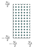
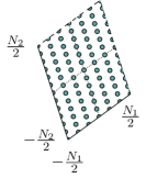
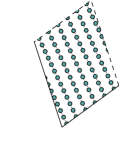
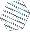
Figure 3: While the usual of a diagonal matrix indtroduces a rectangular grid (most left), the matrix $\mathbf{L}$ of the transformed pattern $\operatorname{\mathcal{P}}_{\mathbf{L}}(\mathbf{M})$ introduces rotation and scaling of the unit cube (left). Furthermore, in such a cell, a rank-1-lattice can be used (right), and it is even possible to use arbitrary shapes like an arbitrary hexagonal shape $\mathcal{S}$ (most right). Dotted lines indicate lines of the basis vectors and all pattern consist of 72 points, whose boundary elements are repeated on the other side (the half circles each).

Definition 3.3.

Let $\mathbf{M}\in\mathbb{Z}^{d\times d}$ be an regular integral matrix and $\mathbf{L}\in\mathbb{R}^{d\times d}$ be a regular matrix. Then the transformed pattern is defined by

$$\operatorname{\mathcal{P}}_{\mathbf{L}}(\mathbf{M})\coloneqq\mathbf{L}\Lambda(\mathbf{M})\cap\mathbf{L}\bigl{[}-\tfrac{1}{2},\tfrac{1}{2}\bigr{)}^{d}.$$

One can even take any set of integer points inside a certain shape $\mathcal{S}$, where the shifts $\mathcal{S}+\mathbf{L}\mathbf{z}$, tile the $\mathbb{R}^{d}$, i.e. for all $\mathbf{y}\in\mathbb{R}^{d}$ exists a unique $\mathbf{z}\in\mathbb{Z}^{d}$ such that $\mathbf{y}-\mathbf{z}\in\mathcal{S}$, e.g see Fig. 3 (most right)

This gives rise to a huge variety of unit cells to model the microscopic periodic media. The transformed patterns $\operatorname{\mathcal{P}}_{\mathbf{L}}(\mathbf{M})$ especially introduce the possibility to take anisotropic cell structures inside the unit cell or RVE into account.

Definition 3.3 can also be interpreted in terms of a coordinate transformation. Consider a regular matrix $(A_{ij})_{i,j}=\mathbf{A}\in\mathbb{R}^{d\times d}$ and transformed coordinates $\tilde{\mathbf{x}}=\mathbf{A}\mathbf{x}$ with $\mathbf{x}\in[-\frac{1}{2},\frac{1}{2})^{d}$. Let $\mathbf{u}(\mathbf{x})$ solve the PDE (8) with stiffness distribution $\mathcal{C}(\mathbf{x})$ and macroscopic strain $\epsilon^{0}$.

By [19, Section 8.3] the displacement $\tilde{\mathbf{u}}(\tilde{\mathbf{x}})$ that solves (8) with transformed

$$\tilde{\mathcal{C}}_{ijkl}(\tilde{\mathbf{x}}) =A_{im}A_{jn}A_{ko}A_{lp}\mathcal{C}_{mnop}(\mathbf{x}),$$

and $\tilde{\epsilon^{0}}=\mathbf{A}^{-T}\epsilon^{0}\mathbf{A}^{-1}$ is connected to $\mathbf{u}(\mathbf{x})$ by $\tilde{\mathbf{u}}(\tilde{\mathbf{x}})=\mathbf{A}^{-\mathrm{T}}\mathbf{u}(\mathbf{x})$. Discretizing $\mathbf{u}(2\pi\mathbf{y})$ with $\mathbf{y}\in\operatorname{\mathcal{P}}(\mathbf{M})$ leads to

$$\mathbf{u}(2\pi\mathbf{y})=\mathbf{A}^{\mathrm{T}}\tilde{\mathbf{u}}(2\pi\mathbf{A}\mathbf{y})=\mathbf{A}^{\mathrm{T}}\tilde{\mathbf{u}}(2\pi\tilde{\mathbf{y}})$$

with $\tilde{\mathbf{y}}=\mathbf{A}\mathbf{y}\in\operatorname{\mathcal{P}}(\mathbf{M})$ or equivalently $\tilde{\mathbf{y}}\in\operatorname{\mathcal{P}}_{\mathbf{A}}(\mathbf{M})$.

Compared to the usual coordinate transform, c.f. [15, 28], to the unit cell, the homogenization on patterns allows for further preference of directions in the cell other than the transformed coordinate axes.

3.4 Convergence of the discretization

Let $n$ be the smallest eigenvalue of $\mathbf{M}$ being larger than $1$, where $\mathbf{M}\in\mathbb{Z}^{d\times d}$. Then interpolation error on the generating set $\operatorname{\mathcal{G}}(\mathbf{M}^{\mathrm{T}})$ can be bounded from above by the diagonal matrix $\tilde{\mathbf{M}}\coloneqq\operatorname{diag}(\lfloor n\rfloor,\ldots,\lfloor n\rfloor)\in\mathbb{Z}^{d\times d}$, because the hypercube $\frac{1}{2}\tilde{\mathbf{M}}[-1,1]^{d}$ is contained in the parallelepiped $\tfrac{1}{2}\mathbf{M}^{\mathrm{T}}[-1,1]^{d}$ which is used to define $\operatorname{\mathcal{G}}(\mathbf{M}^{\mathrm{T}})$ and hence $\operatorname{\mathcal{G}}(\tilde{\mathbf{M}}^{\mathrm{T}})\subset\operatorname{\mathcal{G}}(\mathbf{M}^{\mathrm{T}})$. From any sequence of discretizations $\mathbf{M}_{i}$ whose determinants $m_{i}$ tend to infinity, we also obtain, that the smallest eigenvalue tends to infinity because the matrix has to span the frequency lattice $\mathbb{Z}^{d}$. With this argument the convergence of the such discretization sequence is dominated by a standard case of a Cartesian grid and the convergence proof of e.g. [23] the convergence in this setting follows directly.

4 Geometries and analytic solutions

To examine the effects the pattern matrix has on the solution, this section describes two problems where the effective stiffness tensor and an analytic expression for the strain field are known. The first structure is a laminate which as a basically one-dimensional structure exhibiting straight interfaces and thus a unique dominant direction to analyze. The second geometry we introduce is given by two confocal ellipsoids defining a coated core in a matrix material. The stiffnesses of the involved materials are chosen in such a way that the inclusion acts neutrally with respect to a specific macroscopic strain. This generalizes the (isotropic) Hashin structure [11]. The curved interfaces make it more difficult to sample the structure efficiently and the occurring effects can be expected to be more complex.

4.1 The laminate structure

The probably most simple structure with a predominant direction is a periodic laminate as shown in Fig. 7 ( middle) . This structure consists of two isotropic materials alternating in the direction of lamination $\mathbf{n}\in\mathbb{R}^{d}$ with $\lVert\mathbf{n}\rVert=1$ and being constant perpendicular to it. For this structure Milton [19, Section 9.5] derives an analytic equation for the effective matrix $\mathcal{C}^{\mathrm{eff}}$ that is given by

$$\left(\mathcal{S}-\mathcal{T}\right)^{-1} =\int_{\mathbb{T}^{d}}\left(\tilde{\mathcal{S}}(\mathbf{x})-\mathcal{T}\right)^{-1}\,\mathrm{d}\mathbf{x}$$

with

$$\mathcal{S} \coloneqq\sigma_{0}\left(\sigma_{0}\operatorname{Id}-\mathcal{C}^{\mathrm{eff}}\right)^{-1},\qquad\tilde{\mathcal{S}}(\mathbf{x})\coloneqq\sigma_{0}\left(\sigma_{0}\operatorname{Id}-\mathcal{C}(\mathbf{x})\right)^{-1},$$

$$\mathcal{T}_{ijkl} \coloneqq\frac{1}{2}(n_{i}\delta_{jk}n_{l}+n_{i}\delta_{jl}n_{k}+n_{j}\delta_{ik}n_{l}+n_{j}\delta_{il}n_{k})-n_{i}n_{j}n_{k}n_{l}.$$

The choice of the free parameter $\sigma_{0}$ is explained in [12, Appendix]. Let $\sigma$ be the largest eigenvalue of the spectra of the stiffness tensors $\mathcal{C}(\mathbf{x})$ then a choice of $\sigma_{0}>\sigma$ ensures that all the inversions necessary to solve for $\mathcal{C}^{\mathrm{eff}}$ can be done.

The resulting strain field $\epsilon$ is, like the structure itself, piecewise constant and varies only in the direction of lamination. Let the volume fractions of the two materials be $f_{1}$ and $f_{2}$ with $f_{1}+f_{2}=1$ and call the corresponding constant strain fields $\epsilon^{1}$ and $\epsilon^{2}$. The geometry is constant perpendicular to the direction of lamination. Hence the problem of finding $\epsilon^{1}$ and $\epsilon^{2}$ reduces to a one-dimensional problem. This gives a system of linear equations involving the macroscopic strain $\epsilon^{0}$ to be solved, namely

$$f_{1}\epsilon^{1}+f_{2}\epsilon^{2}=\epsilon^{0},\qquad f_{1}\mathcal{C}^{\mathrm{eff}}\epsilon^{1}+f_{2}\mathcal{C}^{\mathrm{eff}}\epsilon^{2}=\mathcal{C}^{\mathrm{eff}}\epsilon^{0}.$$

4.2 The generalized Hashin structure

The idea of the generalized Hashin structure due to Hashin and Shtrikman [11] is based on constructing a inclusion embedded in a matrix material that acts neural to a specific macroscopic strain, i.e. the inclusion does not effect the surrounding stress field. An example of such an inclusion is the assemblage of coated confocal ellipsoids described by Milton [19, Section 7.7 ff] whose derivation we want to follow. A schematic of such a structure is depicted in Fig. 4, left.

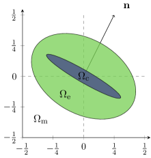
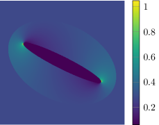
Figure 4: The generalized Hashin structure, $c_{1}=0.05$, $c_{2}=0.35$, $c_{3}=\infty$, $\rho_{\mathrm{c}}=0$, $\rho_{\mathrm{e}}=0.09$, and $\mathbf{n}=(\tfrac{1}{2},1)^{\mathrm{T}}$ in the $xy$-plane, i.e. the 2D setting is shown in a schematic visualization of the material (left) and the analytic solution $\epsilon(\mathbf{x})$ to the elasticity equation (right).

The derivation in Milton is based on an ellipsoid that is aligned with the coordinate axes. An application of [19, Section 8.3] then allows to generalize this to arbitrary orientations resulting in the formulae stated in the following. They allow to predict for a macroscopic strain $\epsilon^{0}$ that will be given below to analytically express the resulting strain field $\epsilon$ and the action of the effective stiffness tensor on this input, $\mathcal{C}^{\mathrm{eff}}\epsilon^{0}$.

To define the geometry consider confocal ellipsoidal coordinates given for $\tilde{\mathbf{x}}\in\mathbb{R}^{3}$ by the equation

$$\frac{\tilde{x}_{1}^{2}}{c_{1}^{2}+\rho}+\frac{\tilde{x}_{2}^{2}}{c_{2}^{2}+\rho}+\frac{\tilde{x}_{3}^{2}}{c_{3}^{2}+\rho}=1$$ (15)

where w.l.o.g. the constants $0\leq c_{1}\leq c_{2}\leq c_{3}\leq\infty$ determine the relative lengths of the semi-axes of the ellipsoid. A constant $\rho\geq-c_{1}^{2}$ specifies the boundary of an ellipsoid where the lengths of the semi-axes are given by $l_{j}(\rho)\coloneqq\sqrt{c_{j}^{2}+\rho}$ with $j=1,2,3$. For a fixed $\tilde{\mathbf{x}}\in\mathbb{R}^{3}$ the ellipsoidal radius $\rho(\tilde{\mathbf{x}})$ is the uniquely determined largest of the possible three solutions of (15) and fulfills $\rho(\tilde{x})\geq-c_{1}^{2}$.

For sake of simplicity, we want to restrict ourselves in this work to prolate spheroids with $c_{1}=c_{2}\leq c_{3}$, oblate spheroids with $c_{1}\leq c_{2}=c_{3}$ and elliptic cylinders. The latter are the limit case $c_{3}\rightarrow\infty$.

For these, according to [19, Section 7.10], the depolarization factors are given by

$$d_{1}(\rho)=d_{2}(\rho),\qquad d_{2}(\rho)=2-2d_{3}(\rho),\qquad d_{3}(\rho)=\frac{1-\delta^{2}}{\delta^{2}}\Bigl{(}\frac{1}{2\delta}\log\Bigl{(}\tfrac{1+\delta}{1-\delta}\Bigr{)}\Bigr{)},$$

for prolate spheroids, where $\delta=\sqrt{1-\tfrac{l_{2}(\rho)^{2}}{l_{3}(\rho)^{2}}}$ . Furthermore we have for oblate spheroids using $\delta=\sqrt{1-\tfrac{l_{1}(\rho)^{2}}{l_{2}(\rho)^{2}}}$ the factors

$$d_{1}(\rho)=\frac{1}{\delta^{2}}\Bigl{(}1-\tfrac{\sqrt{1-\delta^{2}}}{\delta}\sin^{-1}\delta\Bigr{)},\qquad d_{2}(\rho)=2-2d_{1}(\rho),\qquad d_{3}(\rho)=d_{2}(\rho),$$

and finally for elliptic cylinders

$$d_{1}(\rho)=\frac{l_{2}(\rho)}{l_{1}(\rho)+l_{2}(\rho)},\qquad d_{2}(\rho)=\frac{l_{1}(\rho)}{l_{1}(\rho)+l_{2}(\rho)},\qquad d_{3}(\rho)=0.$$

Now let $\rho_{\mathrm{c}}$ and $\rho_{\mathrm{e}}$ be the ellipsoidal radius of the core and the exterior coating, respectively, cf. Fig. 4 (left), with $-c_{1}^{2}<\rho_{\mathrm{c}}<\rho_{\mathrm{e}}$ and with $l_{3}(\rho_{\mathrm{e}})<\frac{1}{2}$ for $c_{3}<\infty$ and $l_{2}(\rho_{\mathrm{e}})<\frac{1}{2}$ for $c_{3}=\infty$, i.e. the exterior ellipsoid should be contained in $[-\frac{1}{2},\frac{1}{2})^{3}$.

Further, let $\mathbf{n}\in\mathbb{R}^{3}$ with $\lVert\mathbf{n}\rVert=1$ be the direction the shortest semi-axis of the ellipsoid with length $l_{1}(\rho)$. Define the rotation matrix that transforms the vector $(1,0,0)^{\mathrm{T}}$ to $\mathbf{n}$ by

$$\mathbf{R}\coloneqq\begin{pmatrix}1&-n_{2}&-n_{3}\\ n_{2}&1&0\\ n_{3}&0&1\end{pmatrix}+\frac{1-n_{1}}{\sqrt{n_{2}^{2}+n_{3}^{2}}}\begin{pmatrix}-n_{2}^{2}-n_{3}^{2}&0&0\\ 0&-n_{2}^{2}&-n_{2}n_{3}\\ 0&-n_{2}n_{3}&-n_{3}^{2}\end{pmatrix}.$$

Then the core, the exterior coating and the surrounding matrix are given by

$$\Omega_{\mathrm{c}} \coloneqq\left\{\mathbf{x}\in\mathbb{R}^{3}:\rho(\mathbf{R}^{-1}\mathbf{x})\leq\rho_{\mathrm{c}}\right\},$$

$$\Omega_{\mathrm{e}} \coloneqq\left\{\mathbf{x}\in\mathbb{R}^{3}:\rho_{\mathrm{c}}<\rho(\mathbf{R}^{-1}\mathbf{x})\leq\rho_{\mathrm{e}}\right\},$$

$$\Omega_{\mathrm{m}} \coloneqq\bigl{[}-\tfrac{1}{2},\tfrac{1}{2}\bigr{)}^{3}\setminus\left(\Omega_{\mathrm{c}}\cup\Omega_{\mathrm{e}}\right),$$

respectively. With

$$f(\rho)\coloneqq\frac{\sqrt{g(\rho_{\mathrm{c}})}}{\sqrt{g(\rho)}}\quad\text{ and }\quad g(\rho)\coloneqq\begin{cases}(c_{1}^{2}+\rho)(c_{2}^{2}+\rho)(c_{3}^{2}+\rho),&\text{for }c_{3}<\infty,\\ (c_{1}^{2}+\rho)(c_{2}^{2}+\rho),&\text{else},\end{cases}$$

the volume fraction of $\Omega_{\mathrm{c}}$ in the coated ellipsoid is given by $f(\rho_{\mathrm{e}})$.

We assume that the material in the core and in the exterior coating behave isotropically, i.e. they are described by stiffness matrices of the form $\mathcal{C}_{ijkl}=\lambda\delta_{ij}\delta_{kl}+\mu(\delta_{ik}\delta_{jl}+\delta_{il}\delta_{jk})$. The parameter $\lambda$ is Lamé’s first parameter and $\mu$ is the shear modulus. We denote the parameters in the core by $\lambda_{\mathrm{c}}$ and $\mu_{\mathrm{c}}$ and in the exterior coating by $\lambda_{\mathrm{e}}$ and $\mu_{\mathrm{e}}$, respectively. Further, the bulk modulus of an isotropic material is given as $\kappa\coloneqq\lambda+\frac{2}{3}\mu$.

Following [19, Section 7.9] we impose a macroscopic strain of

$$\epsilon^{0}=\mathbf{R}\left(\frac{3\kappa_{\mathrm{e}}+4\mu_{\mathrm{e}}}{9(\kappa_{\mathrm{c}}-\kappa_{\mathrm{e}})}\operatorname{Id}+(1-f(\rho_{\mathrm{e}}))\mathbf{S}(\rho_{\mathrm{e}})\right)\mathbf{R}^{\mathrm{T}}$$

with

$$\mathbf{S}(\rho) \coloneqq(1-f(\rho))^{-1}(\mathbf{D}(\rho_{\mathrm{c}})-f(\rho)\mathbf{D}(\rho))\quad\text{ and }\quad\mathbf{D}(\rho)\coloneqq\operatorname{diag}(d_{i}(\rho)_{i=1,2,3}).$$

The effective matrix of the structure and likewise —to ensure the neutrality of the inclusion— the stiffness matrix of the matrix material $\Omega_{\mathrm{m}}$ are given by their action on the macroscopic strain as

$$\mathcal{C}^{\mathrm{eff}}\epsilon^{0}\coloneqq\mathbf{R}\Bigl{(}\tfrac{\kappa_{\mathrm{e}}}{\kappa_{\mathrm{c}}-\kappa_{\mathrm{e}}}(\kappa_{\mathrm{c}}+\frac{4}{3}\mu_{\mathrm{e}})+\frac{4}{3}\mu_{\mathrm{e}}f(\rho_{\mathrm{e}})\Bigr{)}\operatorname{Id}\mathbf{R}^{\mathrm{T}}+\mathbf{R}\frac{2}{3}\mu_{\mathrm{e}}(1-f(\rho_{\mathrm{e}}))(3\mathbf{S}(\rho_{\mathrm{e}})-\operatorname{Id})\mathbf{R}^{\mathrm{T}}.$$

The resulting strain field is then for $\mathbf{x}\in\Omega_{\mathrm{c}}$ given as

$$\epsilon(\mathbf{x})=\mathbf{R}\frac{3\kappa_{\mathrm{e}}+4\mu_{\mathrm{e}}}{9(\kappa_{\mathrm{c}}-\kappa_{\mathrm{e}})}\operatorname{Id}\mathbf{R}^{\mathrm{T}},$$ (16)

and for $\mathbf{x}\in\Omega_{\mathrm{m}}$ as $\epsilon(\mathbf{x})=\epsilon^{0}$, respectively. The strain field is constant in the core and in the matrix material. In the external coating we have for $\mathbf{x}\in\Omega_{\mathrm{e}}$

$$\epsilon(\mathbf{x}) =\mathbf{R}\biggl{(}\tfrac{3\kappa_{\mathrm{e}}+4\mu_{\mathrm{e}}}{9(\kappa_{\mathrm{c}}-\kappa_{\mathrm{e}})}\operatorname{Id}+\mathbf{D}(\rho_{\mathrm{c}})-f(\rho(\tilde{\mathbf{x}}))\mathbf{D}(\rho(\tilde{\mathbf{x}}))+\tfrac{\sqrt{g(\rho_{\mathrm{c}})}}{2}\mathbf{q}(\tilde{\mathbf{x}})\operatorname{\nabla}_{\tilde{\mathbf{x}}}^{T}\rho(\tilde{\mathbf{x}})\biggr{)}\mathbf{R}^{\mathrm{T}},$$

with $$\tilde{\mathbf{x}}\coloneqq\mathbf{R}^{-1}\mathbf{x}$$ and

$$\mathbf{q}(\tilde{\mathbf{x}})_{i} =\frac{\tilde{x}_{i}}{(c_{i}^{2}+\rho(\tilde{\mathbf{x}}))\sqrt{g(\rho(\tilde{\mathbf{x}}))}},\quad\left(\operatorname{\nabla}_{\tilde{\mathbf{x}}}\rho(\tilde{\mathbf{x}})\right)_{i}=\frac{2\tilde{x}_{i}}{c_{i}^{2}+\rho(\tilde{\mathbf{x}})}\Biggl{(}\sum_{j=1}^{3}\frac{\tilde{x}_{i}}{c_{i}^{2}+\rho(\tilde{\mathbf{x}})}\Biggr{)}^{-1},$$

$$i=1,2,3 c_{3}=\infty \mathbf{q}(\tilde{\mathbf{x}})_{3}=0$$. For the case we additionally have ,

$$\left(\operatorname{\nabla}_{\tilde{\mathbf{x}}}\rho(\tilde{\mathbf{x}})\right)_{i} =\frac{2\tilde{x}_{i}}{c_{i}^{2}+\rho(\tilde{\mathbf{x}})}\Biggl{(}\sum_{j=1}^{2}\frac{\tilde{x}_{i}}{c_{i}^{2}+\rho(\tilde{\mathbf{x}})}\Biggr{)}^{-1},\quad i=1,2,\text{ and }\left(\operatorname{\nabla}_{\tilde{\mathbf{x}}}\rho(\tilde{\mathbf{x}})\right)_{3}=0.$$

Example 4.1.

Let an ellipse in 2D be given, i.e. we set the third dimension to be constant by $c_{3}=\infty$, by choosing $c_{1}=0.05$, $c_{2}=0.35$. Choose further $\rho_{c}=0$ and $\rho_{e}=0.09$ and introduce a rotation of $60^{\circ}$ counter clockwise by setting $\mathbf{n}=(\tfrac{1}{2},1,0)^{\mathrm{T}}$. The resulting geometry is shown in  4 (left), the analytic solution $\epsilon(\mathbf{x})$ to the elasticity equation in 4 (right).

5 Numerics

The algorithms used in this paper are implemented in MatLab R2015b in a modular and fast way using vectorization. For the Fourier transform on arbitrary patterns we employ the multivariate periodic anisotropic wavelet library (MPAWL)[4], which was recently ported to Matlab. It uses Matlab’s internal fftn command to apply the fast Fourier transform. All tests were run on a MacBook Pro running Mac OS X 10.11.5, Core i5, 2.6 GHz, with 8 GB RAM using Matlab 2016a and the clang-700.1.76 compiler.

5.1 Hashin

Consider the geometry of the coated ellipsoid as described in Section 4.2 with the parameters in Example 4.1 seen as a two-dimensional problem, i.e. sampled with only one point in $x_{3}$-direction. This structure is strongly orthotropic with the dominant directions being $\mathbf{n}$ and $\mathbf{n}^{\perp}$. To analyze the influence of the sampling matrix $\mathbf{M}$ we compare the relative $\ell^{2}$-error of the strain $\epsilon$ compared with the analytic solution and the relative error in the effective stiffness tensor sampled on $\operatorname{\mathcal{P}}(\mathbf{M})$, i.e we define

$$e_{\ell^{2}}(\mathbf{M})\coloneqq\frac{\lVert\epsilon-\tilde{\epsilon}\rVert_{l^{2}(\operatorname{\mathcal{P}}(\mathbf{M}))}}{\lVert\tilde{\epsilon}\rVert_{l^{2}(\operatorname{\mathcal{P}}(\mathbf{M}))}}\quad\text{ and }\quad e_{\mathrm{eff}}(\mathbf{M})\coloneqq\frac{\lVert\mathcal{C}^{\mathrm{eff}}\epsilon^{0}-\tilde{\mathcal{C}}^{\mathrm{eff}}\epsilon^{0}\rVert_{2}}{\lVert\tilde{\mathcal{C}}^{\mathrm{eff}}\epsilon^{0}\rVert_{2}},$$

where $\epsilon$ and $\mathcal{C}^{\mathrm{eff}}\epsilon^{0}$ are the numerical solutions obtained by Algorithm 1, and $\tilde{\epsilon}$ and $\tilde{\mathcal{C}}^{0}\epsilon^{0}$ are the analytic solutions.

The pattern matrices are parametrized by

$$\mathbf{M}_{j,k,\alpha}\coloneqq\begin{pmatrix}2^{j}&\alpha k&0\\ (1-\alpha)k&2^{14-j}&0\\ 0&0&1\end{pmatrix}$$ (17)

with $j\in\{7,\dots,9\}$, $\alpha\in\{0,1\}$ and $k\in 16\cdot\{-32,\dots,32\}$. For all parameters these matrices have determinant $2^{14}$, i.e. the number of sampling points stays constant. The parameter $k$ shears the pattern, $\alpha$ determines the direction of the shearing and $j$ controls the refinement in the direction of the pattern basis vectors $\mathbf{y}_{j}$, $j=1,\ldots,d_{\mathbf{M}}$, cf. (5). This induces both an anisotropy or preference of direction in the pattern $\operatorname{\mathcal{P}}(\mathbf{M})$ as well as for the basis vectors $\mathbf{h}_{j}$ of the corresponding generating set $\operatorname{\mathcal{G}}(\mathbf{M}^{\mathrm{T}})$, cf. (6), representing the frequencies.

Further, we use pattern matrices of the form

$$\tilde{\mathbf{M}}_{j}\coloneqq\frac{1}{2}\begin{pmatrix}1&1&0\\ -1&1&0\\ 0&0&2\end{pmatrix}\begin{pmatrix}2^{j}&0&0\\ 0&2^{14-j}&0\\ 0&0&1\end{pmatrix}$$

corresponding to a rotation of the grid in the direction of $\mathbf{n}$ with $\det(\tilde{\mathbf{M}}_{j})=2^{13}$.

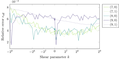
Figure 5: Shear parameter against relative error in the effective stiffness tensor. The corresponding matrices for the curve $(j,\alpha)$ at point $k$ is $\mathbf{M}_{j,k,\alpha}$ from (17). Circles mark the results for matrices $\mathbf{M}_{j,0,0}$ and crosses stand for matrices of the form $\tilde{\mathbf{M}}_{j}$.

In Figure 5 the effect of the shearing parameter $k$ on $e_{\mathrm{eff}}$ is depicted, neglecting curves that do not perform better than $\mathbf{M}_{7,k,\alpha}$ with $\mathbf{M}_{9,k,1}$ as an example for such a curve. For each value of $j$ we choose one color (brightness) and indicate $\alpha=0$ by a solid, $\alpha=1$ by a dotted line, and indicate $\tilde{\mathbf{M}}_{j}$, $j=7,8,9$, by crosses as well as the corresponding diagonal matrices $\mathbf{M}_{j,0,0}=\mathbf{M}_{j,0,1}$ by circles. The circles correspond to the classical rectangular “pixel sampling grid”.

The reference point for the analysis of the results is the unsheared matrix $\mathbf{M}_{7,0,0}$, i.e. the standard equidistant Cartesian grid, giving an error of $3.8\cdot 10^{-3}$. Shearing this matrix in either direction results in a larger errors, e.g.  with twice the error for $\mathbf{M}_{7,-512,0}$ and an error of $5\cdot 10^{-3}$ for $\mathbf{M}_{7,512,0}$.

In contrast $\mathbf{M}_{8,k,0}$ behaves similarly to $\mathbf{M}_{7,k,0}$ with the exception of $k_{-1}=-2^{8}+16$, $k_{0}=16$ and $k_{1}=2^{8}+16$, where the error is $2.4\cdot 10^{-3}$ for the first two and $2.2\cdot 10^{-3}$ for the third point. Note that the matrices possess the same pattern due to $\mathbf{M}_{8,k_{-1},0}\sim_{\operatorname{\mathcal{P}}}\mathbf{M}_{8,k_{0},0}\sim_{\operatorname{\mathcal{P}}}\mathbf{M}_{8,k_{1},0}$.

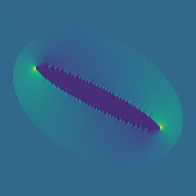
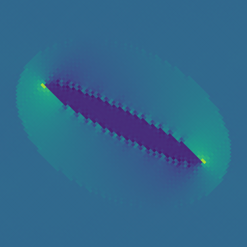
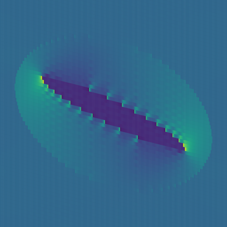
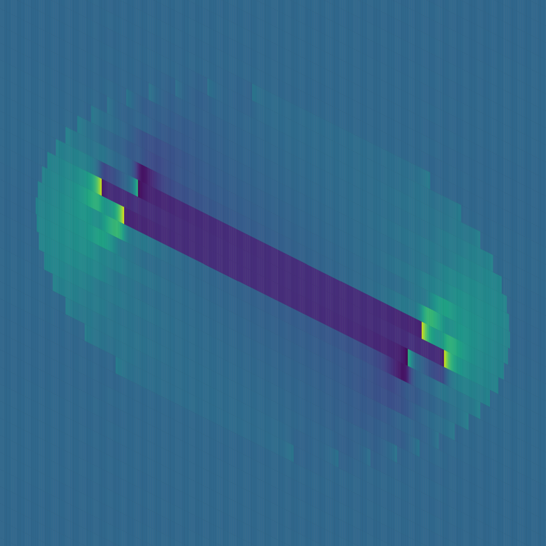
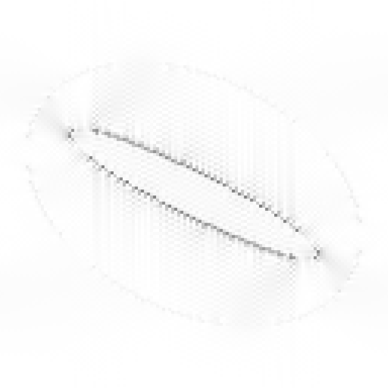
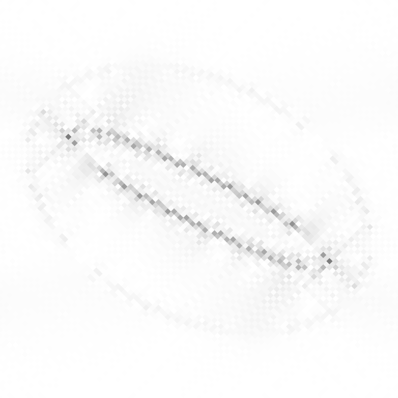
Figure 6: The strain field $\epsilon_{11}$ (first row) using the colormap above and its corresponding $e_{\log}$-error (second row) given by $e_{\log}=\log(1+\lvert\epsilon-\tilde{\epsilon}\rvert)$ using the colormap below. The matrices inducing the sampling pattern points are (left to right): $\mathbf{M}_{7,0,0}=\bigl{(}\begin{smallmatrix}2^{7}&0\\ 0&2^{7}\end{smallmatrix}\bigr{)}$, $\tilde{\mathbf{M}}_{7}=\bigl{(}\begin{smallmatrix}2^{6}&2^{6}\\ -2^{6}&2^{6}\end{smallmatrix}\bigr{)}$, $\mathbf{M}_{8,16,0}=\bigl{(}\begin{smallmatrix}2^{8}&0\\ 2^{4}&2^{6}\end{smallmatrix}\bigr{)}$, and $\mathbf{M}_{9,16,0}=\bigl{(}\begin{smallmatrix}2^{9}&0\\ 2^{4}&2^{5}\end{smallmatrix}\bigr{)}$.

This effect is even more dominant for $\mathbf{M}_{9,k,0}$ that gives an error of around $6\cdot 10^{-3}$ almost everywhere except for $k=-2^{9}+16$ and $k=16$ where it drops to $1.5\cdot 10^{-3}$. These matrices are also congruent with respect to pattern congruence $\sim_{\operatorname{\mathcal{P}}}$.

The strain field and the pointwise error for the $\epsilon_{11}$-component of $\mathbf{M}_{7,0,0}$ are depicted in Fig. 6, first column. As the ellipsoid is not aligned with the pattern, the interface along the long side of the ellipsoid is not resolved well. As the sine functions are not perpendicular to this interface the Gibbs phenomenon dominates the $\ell^{2}$-error. Likewise the strain peak at the tip of the ellipsoid is not captured correctly and worsens $e_{\mathrm{eff}}$ tremendously.

If we choose a matrix with a certain shear, e.g. $\mathbf{M}_{8,16,0}$, where the strain $\epsilon_{11}$ and the corresponding error are shown in Fig. 6 (third column) , we obtain a quite small error in the effective stiffness tensor and resolve the strain peaks correctly. As the pattern, however, is not aligned with the ellipsoid, the interfaces show large errors and inwards and outwards facing corners result in a very large $\ell^{2}$-error.

For the matrices $\mathbf{M}_{9,-2^{9}+16,0}$ and $\mathbf{M}_{9,16,0}$ the pattern is sheared in such a way that it is aligned with the ellipsoid, c.f. Fig. 6, last column, refined in along the longer semi-axis. The strain field $\epsilon_{11}$ is characterized by slowly changing values in the direction of the shorter semi-axis and especially rapidly changing and high strains at the tips of the inner ellipsoid. Therefore, to get small errors, we need only few points in the direction of the shorter semi-axis, in this case only $32$ points. The high strains at the tips of the ellipsoid, however, require a high resolution like $512$ sampling points in this case. This leads to a lower approximation of the edges orthogonal to the smaller semi-axis and hence the Gibbs phenomenon increases the $\ell^{2}$-norm, cf. Fig. 6, first column, for the log-error. This effect concentrates around the tips of the ellipsoid resulting in a core almost shaped like a rectangle. The averaging done to compute the effective stiffness tensor cancels these errors and does therefore not influence the error.

$\mathbf{M}$	$e_{\mathrm{eff}}(\mathbf{M})$	$e_{\ell^{2}}(\mathbf{M})$
$\mathbf{M}_{7,0,0}$	0.0038	0.043
$\tilde{\mathbf{M}}_{7}$	0.0034	0.047
$\mathbf{M}_{8,-2^{8}+16,0}$	0.0024	0.054
$\mathbf{M}_{8,16,0}$	0.0024	0.050
$\mathbf{M}_{8,2^{8}+16,0}$	0.0023	0.048
$\mathbf{M}_{9,-2^{9}+16,0}$	0.0015	0.054
$\mathbf{M}_{9,15,0}$	0.0019	0.052
$\mathbf{M}_{9,16,0}$	0.0015	0.054
$\mathbf{M}_{9,17,0}$	0.0024	0.054
$\mathbf{M}_{7,2^{8},1}$	0.0038	0.023
$\mathbf{M}_{7,2^{8}+16,1}$	0.0036	0.022

Table 1: Relative effective stiffness and $\ell^{2}$-errors for several shearing matrices. While matching the direction, $\mathbf{M}_{9,16,0}$ reduces the $e_{\text{eff}}$ error, the $e_{\ell^{2}}$-error is reduced tremendously by e.g. shearing the standard grid. This can be seen by looking at $\mathbf{M}_{7,2^{8}+16,1}$.

Table 1 shows both the $\ell^{2}$- and the $e_{\mathrm{eff}}$-errors for several matrices. The smallest value of $e_{\mathrm{eff}}$ is reached for $\mathbf{M}_{9,-2^{9}+16,0}$ and $\mathbf{M}_{9,16,0}$. The error for shear parameters around $\mathbf{M}_{9,16,0}$ get slightly worse by changing to $k=15$ or $k=17$, respectively. The smallest $\ell^{2}$-errors can be obtained by $\mathbf{M}_{7,2^{8},1}$ and $\mathbf{M}_{7,2^{8}+16,1}$, giving errors only half as large as in the standard case. The pattern $\mathbf{M}_{7,2^{8},1}$ involves taking a standard pixel grid for sampling and then shearing the unit cell in such a way that it is aligned with the ellipsoid. This gives a balance between resolving the interfaces and capturing the strain peak. The alignment of the sine ansatz functions with the ellipsoid reduces the Gibbs phenomenon and the comparatively large number of frequencies used in the direction of the strain peaks allows for small errors there. The matrix $\mathbf{M}_{7,2^{8}+16,1}$ further shears the pattern by a small amount and resolves the strain peak better while preserving the good resolution of the ellipsoid.

Subsampling of the complete rectangular grid of one $\mathbf{M}_{j,0,0}$ on the so-called quincunx pattern induced by the matrix $\tilde{\mathbf{M}}_{j}$ shown as circles for the former and crosses for the latter matrices in Fig. 5, gives slightly smaller values of $e_{\mathrm{eff}}$. The $\ell^{2}$-errors like for $\tilde{\mathbf{M}}_{7}$, cf. Figs. 6, second column, also decrease even especially when taking into account that only half the sampling values are used.

5.2 Subsampling

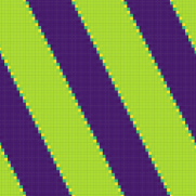
Figure 7: A comparison of 3 different sampling sets of the laminate material: a full $64\times 64$ (left, $e_{\ell^{2}}(\mathbf{M}_{a})=0.109$, 94 Iterations), an adapted rank-1-lattice having $64$ points (middle, $e_{\ell^{2}}(\mathbf{M}_{b})=0.0348$, 9 It.) and the comparison pixel grid also having $64$ points, i.e. $8\times 8$ pixel (right, $e_{\ell^{2}}(\mathbf{M}_{c})=0.2909$, 89 It.). The latter two are both subsamplings of the first.

We study possibilities to subsample given (large) data, when certain directional information is given, e.g. the laminate from Section 4.1 and a given normal vector of $\mathbf{n}=(1,\tfrac{1}{2})^{\mathrm{T}}$. We choose a matrix $\mathbf{N}$ being a factorization of a pixel grid and of the form

$$\mathbf{M}=\begin{pmatrix}a&0\\ 0&a\end{pmatrix}=\begin{pmatrix}1&-\frac{a}{2}\\ 0&a\end{pmatrix}\begin{pmatrix}a&\frac{a}{2}\\ 0&1\end{pmatrix}\eqqcolon\mathbf{J}\mathbf{N}$$

and hence $\operatorname{\mathcal{P}}(\mathbf{N})\subset\operatorname{\mathcal{P}}(\mathbf{M})$ if $\frac{a}{2}$ is an integer. Note that in the sub pattern the most dominant direction in the Fourier domain is the direction orthogonal to the edge direction. Setting $a=2^{6}$ the pixel sampling contains just $2^{12}=4096$ data items, a size where the dominant numerical effects like the Gibbs phenomenon can still be observed. We compare the following patterns: first we sample on the full grid, i.e. we choose $\mathbf{M}_{\text{a}}=\bigl{(}\begin{smallmatrix}64&0\\ 0&64\end{smallmatrix}\bigr{)}$. We consider a directional sub lattice given by $\mathbf{M}_{\text{b}}=\bigl{(}\begin{smallmatrix}64&32\\ 0&1\end{smallmatrix}\bigr{)}$ following the construction above and resulting in $64$ data points, only the square root of the number of points of the full grid. By construction we have $\operatorname{\mathcal{P}}(\mathbf{M}_{\text{b}})\subset\operatorname{\mathcal{P}}(\mathbf{M}_{\text{a}})$ and that the spanning vector $\mathbf{y}_{1}$ of this rank-$1$-lattice, is orthogonal to the edges present in the material. This can for example be done by examining the large(r) dataset with respect to its edge directions and subsampling accordingly. We study the effect of these in contrast to $\mathbf{M}_{\text{c}}=\bigl{(}\begin{smallmatrix}8&0\\ 0&8\end{smallmatrix}\bigr{)}$ having also $64$ points. Clearly this is also a sub lattice of $\mathbf{M}_{\text{a}}$. We employ Algorithm 1 and a Chauchy criterion for stopping, i.e. $\tfrac{\lVert\epsilon^{(n+1)}-\epsilon^{(n)}\rVert}{\lVert\epsilon^{(0)}\rVert}$ with a threshold of $10^{-9}$. The results are shown in Figure 7.

The full grid based approach of $\mathbf{M}_{\text{a}}$ shown in Fig. 7 (left) suffers from the well known Gibbs phenomenon. The subsampling on $\operatorname{\mathcal{P}}(\mathbf{M}_{\text{b}})$ in Fig 7 (middle) reduces the number of iterations tremendously from $94$ to only $9$ and the computational times from $41.2$ to only $4.5$ seconds. This is not the case for the pixel grid subsampling given by $\operatorname{\mathcal{P}}(\mathbf{M}_{\text{c}})$ shown in Fig 7 (right) which still requires $89$ iterations and $46.1$ seconds.

Looking at the $\ell^{2}$-error depicted in the captions of Fig. 7, reducing the number of points from $64^{2}$ in $\operatorname{\mathcal{P}}(\mathbf{M}_{a})$ to $64$ in $\operatorname{\mathcal{P}}(\mathbf{M}_{b})$ also reduces the error by a factor of roughly 3.1. The tensor pixel grid of $\mathbf{M}_{\text{c}}$ with $8\times 8=64$ is by a factor of $8$ worse than our new anisotropic approach given by $\mathbf{M}_{b}$.

Finally, we analyse the error of the effective stiffness $e_{\text{eff}}(\mathbf{M}_{x})$, $x\in\{a,b,c\}$. The values are $e_{\text{eff}}(\mathbf{M}_{a})=0.0042$, $e_{\text{eff}}(\mathbf{M}_{b})=0.0134$, and $e_{\text{eff}}(\mathbf{M}_{c})=0.0495$. Hence having only $64$ times the number of points as $\operatorname{\mathcal{P}}(\mathbf{M}_{\text{b}})$ the first example is only about a factor of $3.2$ times better. This pattern yields an error that is by a factor of roughly $3.6$ smaller than the tensor product grid $\operatorname{\mathcal{P}}(\mathbf{M}_{c})$ having the same number of points.

In total, such a construction is also possible for other integer values, though the factorization might not be that easy to find. Other normal vector directions can be approximated, e.g. applying the dyadic decomposition in frequency as in [3, Chapter 4]. Then, the direction to be approximated by the factorization of the matrix $\mathbf{M}$ has to be orthogonal to the direction, which should be sampled the most dense, i.e. for the laminate this direction of interest in the Fourier domain is along the laminate.

6 Summary and Conclusion

This article generalizes the discretization of the Lippmann-Schwinger equation and the resulting numerical algorithm to anisotropic sampling lattices. This allows to refine other directions than the coordinate axes, even supporting non-orthogonal refinement. This leads to smaller errors in the strain field and a better approximation of the effective stiffness tensor when taking the anisotropic properties of a material into account. Furthermore, the orientation of the sine functions for the real-valued discrete Fourier transform can be chosen. This allows for alignment of the ansatz functions with interfaces and increases their resolution while reducing the Gibbs phenomenon. Especially regions and directions of high strain can thus be resolved better. We show that these additional choices can not be reproduced by linear transformations of the problem, e.g. rotations of the geometry. Subsampling on suitable patterns makes these techniques also accessible for data given on standard Cartesian grids present in many applications.

The application of the corresponding fast Fourier transform on patterns does not increase the computational effort and might even be computationally advantageous in case of lattices of rank 1. In this case the Fast Fourier transform reduces to a one-dimensional transform, greatly reducing the computational complexity required of the FFT algorithm. Other modifications applied to the Basic scheme of Moulinec and Suquet can still be applied to the anisotropic lattice version introduced in this paper. These modifications include adaptions of the numerical algorithm to increase both robustness and speed. Furthermore, schemes stemming from finite difference or finite element methods can also be incorporated into the anisotropic setting.

An open problem that has to be studied in detail is an automatically performed choice of the pattern matrix $\mathbf{M}$. While the currently chosen matrices already stem from geometric interpretation of how to choose the directions of interest in the sampling lattice, the choice is up to now manually done. An analysis of the main directions of interfaces may provide a good selection of a pattern, but there may be additional restraints to take into account when selecting a sampling scheme.

Acknowledgment

The authors would like to thank Bernd Simeon and Gabriele Steidl for their idea to start this collaboration.

References

- Åhlander and Munthe-Kaas [2005] K. Åhlander, H. Munthe-Kaas, Applications of the generalized fourier transform in numerical linear algebra, BIT Num. Math. 45 (2005) 819–850. doi:10.1007/s10543-005-0030-3.
- Bergmann [2013a] R. Bergmann, The fast Fourier transform and fast wavelet transform for patterns on the torus, Appl. Comp. Harmon. Anal. 35 (2013a) 39–51. doi:10.1016/j.acha.2012.07.007.
- Bergmann [2013b] R. Bergmann, Translationsinvariante Räume multivariater anisotroper Funktionen auf dem Torus, Dissertation, Universität zu Lübeck, 2013b. URL: http://www.math.uni-luebeck.de/mitarbeiter/bergmann/publications/diss_bergmann.pdf.
- Bergmann [2014] R. Bergmann, The multivariate periodic anisotropic wavelet library, 2014. URL: http://library.wolfram.com/infocenter/MathSource/8761/.
- Bergmann and Prestin [2014a] R. Bergmann, J. Prestin, Multivariate anisotropic interpolation on the torus, in: Approximation Theory XIV: San Antonio 2013, Springer International Publishing, Cham, 2014a, pp. 27–44. doi:10.1007/978-3-319-06404-8_3.
- Bergmann and Prestin [2014b] R. Bergmann, J. Prestin, Multivariate periodic wavelets of de la Vallée Poussin type, J. Fourier. Anal. Appl. 21 (2014b) 342–369. doi:10.1007/978-3-319-06404-8_3.
- de Boor et al. [1993] C. de Boor, K. Höllig, S. Riemenschneider, Box Splines, Springer-Verlag, New York, 1993. doi:10.1007/978-1-4757-2244-4.
- Chui and Li [1994] C.K. Chui, C. Li, A general framework of multivariate wavelets with duals, Appl. Comp. Harmon. Anal. 1 (1994) 368–390. doi:10.1006/acha.1994.1023.