General formulation of coupled radiative and conductive heat transfer between compact bodies

Abstract

We present a general framework for studying strongly coupled radiative and conductive heat transfer between arbitrarily shaped bodies separated by sub-wavelength distances. Our formulation is based on a macroscopic approach that couples our recent fluctuating volume–current (FVC) method of near-field heat transfer to the more well known Fourier conduction transport equation. We apply our technique to consider heat exchange between aluminum-zinc oxide nanorods and show that the presence of bulk plasmon resonances can result in extremely large radiative heat transfer rates (roughly twenty times larger than observed in planar geometries), whose interplay with conductive transport leads to nonlinear temperature profiles along the nanorods.

Radiative heat transfer (RHT) between objects held at different temperatures can be many orders of magnitude larger in the near field (short separations $d\ll$ thermal wavelength $\lambda_{T}=\hbar c/k_{\mathrm{B}}T$) than for far-away objects Basu et al. (2009); Volokitin and Persson (2007); Ottens et al. (2011); Reid et al. (2013); Song et al. (2015a). Recently, we showed that that the interplay of near-field RHT and conduction in planar geometries can dramatically modify the temperature and thermal exchange rate at sub-micron separations Messina et al. (2016). Such strongly-coupled conduction–radiation (CR) phenomena are bound to play a larger role in situations involving structured materials, where RHT can be further enhanced Miller et al. (2015); Liu and Shen (2015); Phan et al. (2013); Yang and Wang (2016); Biehs et al. (2012); Dai et al. (2015) and modified Rodriguez et al. (2013, 2012); Edalatpour and Francoeur (2016); Rodriguez et al. (2011), and in on-going experiments exploring nanometer scale gaps, where the boundary between conductive (phonon- and electron-mediated) and radiative transport begins to blurr Cahill et al. (2014); Chiloyan et al. (2015).

We present a general CR framework that captures the interplay of near-field RHT and thermal conduction along with the existence of large temperature gradients in arbitrary geometries. We show that under certain conditions, i.e. materials and structures with separations and geometric lengthscales in the nanometer range, RHT can approach and even exceed conduction, significantly changing the stationary temperature distribution of heated objects. Our approach is based on a generalization of our recent fluctuating volume-current (FVC) formulation of electromagnetic (EM) fluctuations, which when coupled to the more standard Fourier heat equation describing conductive transport at macroscopic scales, allows studies of CR between arbitrary shapes, thereby generalizing our prior work with slabs Messina et al. (2016). As a proof of concept, we consider an example geometry involving aluminum-zinc oxide (AZO) nanorods separated by vacuum gaps, which exhibits more than an order of magnitude enhancement in RHT compared to planar slabs, and hence leads to even larger temperature gradients. We find that while RHT between thin slabs is primarily mediated by surface modes, resulting in linear temperature gradients, the presence of bulk nanorod resonances leads to highly distance-dependent nonlinear temperature profiles.

Coupled radiative and conductive diffusion processes in nanostructures are becoming increasingly important Joulain (2008); Chiloyan et al. (2015), with recent works primarily focusing on the interplay between thermal diffusion and external optical illumination such as laser-heating of plasmonic structures Baffou et al. (2010, 2014); Ma et al. (2014); Baldwin et al. (2014); Biswas and Povinelli (2015). On the other hand, while it is known that conduction has a strong influence on RHT experiments St-Gelais et al. (2016, 2014), the converse has thus far been largely unexplored because RHT is typically too small to result in appreciable temperature gradients Wong et al. (2011, 2014); Lau et al. (2016). However, our recent work Messina et al. (2016) suggests that such an interplay can be significant at tens of nanometer separations and in fact may already have been present (though overlooked) in recent experiments involving planar systems Shen et al. (2009); Kittel et al. (2005); Kim et al. (2015); Song et al. (2015b). Moreover, since planar structures are known to exhibit highly suboptimal RHT rates Miller et al. (2015), we expect even stronger interplays in more complex geometries, such as metasurfaces Liu and Zhang (2015), hyperbolic metamaterials Liu et al. (2014); Biehs et al. (2012), or lattices of metallic antennas Liu and Shen (2015); Miller et al. (2015).

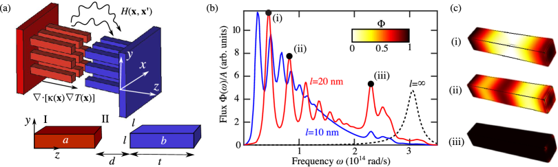
Figure 1: (a) Schematic illustration of two square lattices of nanorods (labelled $a$ and $b$) of thickess $t$, period $\Lambda$, cross-sectional area $l\times l$, and separation $d$, whose temperature distribution and energy exchange is mediated by both conductive $\nabla\cdot[\kappa(\mathbf{x})T(\mathbf{x})]$ and radiative $H(\mathbf{x},\mathbf{x}^{\prime})$ heat transfer. (b) Total radiative heat transfer spectrum $\Phi(\omega)$ between two AZO nanorods (solid lines) of thickness $t=500$ nm and cross-sectional area $A=l^{2}$, separated by $d=20$ nm and held at temperatures $T_{a(b)}=800(300)$ K. The spectrum is shown for different cross-sections $l=\{10,20\}$ nm (blue and red lines) and in the limit $l=\infty$, corresponding to two planar slabs. (c) Spatial radiative heat flux in nanorod $a$ for the case $l=20$ nm, corresponding to the (i) first, (ii) second, and (iii) SPP plasmon resonances, respectively, annotated in (b).

Formulation.— In what follows, we describe a general formulation of coupled CR applicable to arbitrary geometries. Consider a situation involving two bodies (the same framework can be extended to multiple bodies), labelled $a$ and $b$, subject to arbitrary temperature profiles and exchanging heat among one other, shown schematically in Fig. 1(a). Neglecting convection and considering bodies with lengthscales larger or of the order of their phonon mean-free path, in which case Fourier conduction is valid, the stationary temperature distribution satisfies:

$$\nabla\cdot[\kappa(\mathbf{x})\nabla T(\mathbf{x})]+\int\mathrm{d}^{3}\mathbf{x}^{\prime}\,H(\mathbf{x},\mathbf{x}^{\prime})=Q(\mathbf{x})$$ (1)

where $\kappa(\mathbf{x})$ and $Q(\mathbf{x})$ describe the bulk Fourier conductivity and presence of some external heat source at $\mathbf{x}$, respectively, and $H(\mathbf{x},\mathbf{x}^{\prime})$ denotes the radiative power per unit volume from $\mathbf{x}^{\prime}$ to $\mathbf{x}$.

Our ability to compute $H(\mathbf{x},\mathbf{x}^{\prime})$ in full generality hinges on an extension of a recently introduced FVC method that exploits powerful EM scattering techniques Polimeridis et al. (2015) to enable fast calculations of RHT under arbitrary geometries and temperature distributions. The starting point of this method is the volume-integral equation (VIE) formulation of EM, in which the scattering unknowns are 6-component polarization currents $\xi$ in the interior of the bodies coupled via the homogeneous $6\times 6$ Green’s function $\Gamma$ of the intervening medium Polimeridis et al. (2015). Given two objects described by a susceptibility tensor $\chi(\mathbf{x})$ and a Galerkin decomposition of the induced currents $\xi=\sum_{i}x_{i}b_{i}$, with $\{b_{i}\}$ denoting localized basis functions throughout the objects ($i$ is the global index for all bodies), the scattering of an incident field due to some fluctuating current-source $\sigma=\sum_{i}s_{i}b_{i}$ can be determined via solution of a VIE equation, $x+s=Ws$, in terms of the unknown and known expansion coefficients $\{x_{i}\}$ and $\{s_{i}\}$, respectively, where $W^{-1}_{i,j}=\langle b_{i},(I+i\omega\chi G)b_{j}\rangle$ and $G_{i,j}=\langle b_{i},\Gamma\star b_{j}\rangle$ are known as VIE and Green matrices Polimeridis et al. (2015). Previously, we exploited this formalism to propose an efficient method for computing the total heat transfer between any two compact bodies Polimeridis et al. (2015), based on a simple voxel basis expansion (uniform discretization). The solution of (1) requires an extension of the FVC method to include the spatially resolved heat transfer between any two voxels, which we describe below.

Consider a fluctuating current-source $\sigma_{\alpha}=s_{\alpha}b_{\alpha}$ at $\mathbf{x}_{a}=b_{\alpha}$ in a body $a$. Such a “dipole” source induces polarization–currents $\xi_{\beta}=x_{\beta}b_{\beta}$ and EM fields $\phi_{\beta}$ throughout space in body $b$ (and elsewhere), such that the heat flux at $\mathbf{x}_{b}=b_{\beta}$ is given (by Poynting’s theorem) by:

$$\Phi(\omega;\mathbf{x}_{a}\rightarrow\mathbf{x}_{b})=\frac{1}{2}\langle\operatorname{Re}\left(\xi_{\beta}^{*}\phi_{\beta}\right)\rangle$$ (2)

where “$\langle\ldots\rangle$” denotes a thermodynamic ensemble average. Expressing the polarization–currents and fields in the localized basis $\{b_{\alpha}\}$, and exploiting the volume equivalence principle to express the field as a convolution of the incident and induced currents with the vacuum Green’s function (GF), $\phi=\Gamma\star(\xi+\sigma)$, one finds that (2) can be expressed in a compact, algebraic form involving VIE matrices:

$$\Phi(\omega;\mathbf{x}_{a}\rightarrow\mathbf{x}_{b}) =\frac{1}{2}\langle\operatorname{Re}\left\{x_{\beta}^{*}[G(x+s^{\alpha})]_{\beta}\right\}\rangle$$

$$=\frac{1}{2}\langle\operatorname{Re}\left\{(x+s^{\alpha})_{\beta}^{*}[G(x+s^{\alpha})]_{\beta}\right\}\rangle$$

$$=\frac{1}{2}\langle\operatorname{Re}\left[(Ws^{\alpha})_{\beta}^{*}(GWs^{\alpha})_{\beta}\right]\rangle$$

$$=\frac{1}{2}\operatorname{Re}\left[D_{\alpha,\alpha}W^{\dagger}_{\alpha,\beta}(GW)_{\beta,\alpha}\right]$$ (3)

where $s^{\alpha}$ is a vector that is zero everywhere except at the $\alpha$th element, denoted by $s_{\alpha}$, and ${D}_{\alpha,\beta}=\langle s_{\alpha}^{*}s_{\beta}\rangle=\int\int d^{3}\mathbf{x}\,d^{3}\mathbf{y}\,b_{\alpha}^{\ast}(\mathbf{x})\langle\sigma(\mathbf{x})\sigma^{\ast}(\mathbf{y})\rangle b_{\beta}(\mathbf{y})$ is a real, diagonal matrix encoding the thermodynamic and dissipative properties of each object Polimeridis et al. (2015) and described by the well-known fluctuation–dissipation theorem, $\langle\sigma_{i}(\mathbf{x},\omega)\sigma_{j}^{\ast}(\mathbf{y},\omega)\rangle=\frac{4}{\pi}\omega\operatorname{Im}\epsilon(\mathbf{x},\omega)\Theta(T_{\mathbf{x}})\delta(\mathbf{x}-\mathbf{y})\delta_{ij}$, where $\Theta(T)=\hbar\omega/[\mathrm{exp}(\hbar\omega/k_{b}T)-1]$ is the Planck distribution. It follows then that the heat flux emitted or absorbed at a given position $\mathbf{x}_{a}$, the main quantity entering (1) through $\int\mathrm{d}^{3}\mathbf{x}^{\prime}\,H(\mathbf{x},\mathbf{x}^{\prime})=\int\mathrm{d}\omega\,\Phi(\omega;\mathbf{x})$, is given by:

$$\Phi(\omega;\mathbf{x}_{a}) =\int_{V_{b}}\mathrm{d}^{3}\mathbf{x}_{b}\left[\Phi(\omega;\mathbf{x}_{b}\rightarrow\mathbf{x}_{a})-\Phi(\omega;\mathbf{x}_{a}\rightarrow\mathbf{x}_{b})\right]$$

$$=\frac{1}{2}\text{Tr }_{\beta|b_{\beta}\in V_{b}}\operatorname{Re}\left[D_{\beta,\beta}W^{\dagger}_{\beta,\alpha}(GW)_{\alpha,\beta}-(\alpha\leftrightarrow\beta)\right]$$

$$=\frac{1}{2}\operatorname{Re}\left[\underbrace{GWD^{b}W^{\dagger}}_{\Phi_{\mathrm{a}}}-\underbrace{DW^{\dagger}P^{b}GW}_{\Phi_{\mathrm{e}}}\right]_{\alpha,\alpha}$$ (4)

Here, $P^{a(b)}$ denotes the projection operator that selects only basis functions in $a(b)$, such that $D^{b}=P^{b}DP^{b}$ is a diagonal matrix involving only fluctuations in object $b$. Furthermore, the first (second) term in (4) describe the absorbed (emitted) power in $\mathbf{x}_{a}$, henceforth denoted via the subscript “a(e)”.

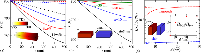
Figure 2: (a) Temperature profile along the $z$ coordinate of a nanorod (solid lines) when it is heated from one side to a temperature of 800 K, and is separated from an identical, constant- and uniform-temperature nanrod held at $T=300$ K on the other side, by a gap size $d=20$ nm. The nanorods have cross-sectional width $l=10$ nm and thicknesses $t=500$ nm, and are made up of AZO with results shown for multiple values of the doping concentration $\{2,6,11\}\mathrm{wt}\%$ (blue, red, and black lines). Also shown are the temperature profiles of slabs (dashed lines) of the same thickness (corresponding to the limit $l\to\infty$). (Inset:) Temperature distribution throughout the nanorod in the case of $11\mathrm{wt}\%$. (b) Temperature profiles of nanorods of width $l=20$ nm under various separations $d=\{5,10,20,30\}$ nm (black, blue, red, and green lines). (c.inset:) The ratio of total radiative heat flux for nanorods of width $l=20$ nm to that of the slabs as a function of $d$, in the presence (red dots) or absence (black dots) of temperature gradients induced by conduction and radiation interplay, with the flux value shown in (c), for nanorods (red) and slabs (blue), also in the presence (solid lines) or absence (dashed lines) of temperature gradients induced by the interplay of conduction and radiation.

Equation 4 is a generalization of our previous expression for the total heat transfer between two arbitrary inhomogeneous objects Polimeridis et al. (2015) in that it includes both the spatially resolved absorbed and emitted power throughout the entire geometry. In Polimeridis et al. (2015), we showed that the low-rank nature of the GF operator enables truncated, randomized SVD factorizations and therefore efficient evaluations of the corresponding matrix operations. We find, however, that in this case, the inclusion of the absorption term does not permit such a factorization, except in special circumstances. In particular, writing down the two terms separately by expanding into the subspace spanned by each object, we find:

$$\Phi_{\mathrm{a}}(\omega;\mathbf{x}_{a}) =\frac{1}{2}\operatorname{Re}\left[G^{ab}W^{bb}D^{bb}W^{ab\dagger}+G^{aa}W^{ab}D^{bb}W^{ab\dagger}\right]$$ (5)

$$\Phi_{\mathrm{e}}(\omega,\mathbf{x}_{a}) =-\frac{1}{2}\left[\operatorname{Re}(D^{aa}W^{ba\dagger}G^{ba}W^{aa})\right.$$

$$\hskip 50.58878pt\left.+D^{aa}W^{ba\dagger}\operatorname{sym}(G^{bb})W^{ba}\right]_{\alpha,\alpha}$$ (6)

with $X^{ij}=P^{i}XP^{j}$ denoting the sub-block of matrix $X$ connecting basis functions in object $i$ to object $j$, and $\operatorname{sym}X=\frac{1}{2}(X+X^{\dagger})$ denoting the symmetric part of $X$.

Equation 6, describing emission, can be evaluated efficiently because the matrices $G^{ba}$ and $\operatorname{sym}{G^{bb}}$ are both low rank ($\ell\ll N$) Polimeridis et al. (2015), in which case they can be SVD factorized to allow fast matrix multiplications. It follows that the total heat transfer, i.e. the trace of (6), can also be computed efficiently. Unfortunately, the second term of (5) involves both the symmetric and anti-symmetric parts of $G^{aa}$, the latter of which is full rank. More conveniently, detailed balance dictates that $\Phi(\omega;\mathbf{x}_{b}\rightarrow\mathbf{x}_{a})=\Phi(\omega;\mathbf{x}_{a}\rightarrow\mathbf{x}_{b})$ whenever $T(\mathbf{x}_{a})=T(\mathbf{x}_{b})$, which implies that $\operatorname{Re}\left[M_{\beta,\beta}W^{\dagger}_{\beta,\alpha}(GW)_{\alpha,\beta}\right]=\operatorname{Re}\left[M_{\alpha,\alpha}W^{\dagger}_{\alpha,\beta}(GW)_{\beta,\alpha}\right]$, where $M_{\alpha,\alpha}=\operatorname{Im}\varepsilon(\mathbf{x}_{\alpha},\omega)$ is a real, diagonal matrix encoding the dissipative properties of the bodies, leading to the following modified expression for the absorption rate:

$$\Phi_{\mathrm{a}}(\omega;\mathbf{x}_{a}) =\frac{1}{2}\left[\operatorname{Re}(M^{aa}W^{ba\dagger}K^{bb}G^{ba}W^{aa})\right.$$

$$\hskip 50.58878pt\left.+M^{aa}W^{ba\dagger}\operatorname{sym}(K^{bb}G^{bb})W^{ba}\right]_{\alpha,\alpha}$$ (7)

where the real and diagonal matrix $K_{\alpha,\alpha}=D_{\alpha,\alpha}/M_{\alpha,\alpha}$ is only relevant to the Plank function $\Theta(T(\mathbf{x}_{\alpha}),\omega)$. Noticeably, the symmetrized operator in the second term is full rank except whenever the temperature of object $b$ is close to uniform, in which case $\operatorname{sym}(K^{bb}G^{bb})\approx K^{bb}\operatorname{sym}G^{bb}$. While solution of (7) is feasible, it remains an open problem to find a formulation that allows fast evaluations of the spatially resolved absorbed power under arbitrary temperature distributions.

Given (4), one can solve the coupled CR equation in any number of ways Press (2007). Here, we exploit a fixed-point iteration procedure based on repeated and independent evaluations of (3) and (1), converging once both quantities approach a set of self-consistent steady-state values. Equation 1 is solved via a commercial, finite-element heat solver whereas (3) is solved through a free, in-house implementation of our FVC method Polimeridis et al. (2015). While the above formulation is general, below we explore the computationally convenient situation in which object $b$ is kept at a constant, uniform temperature by means of a carefully chosen thermal reservoir, such that the absorbed power in object $a$ can be computed efficiently via (7). Furthermore, absorption can be altogether ignored whenever one of the bodies is heated to a much larger temperature than the other (as is the case below). The power emitted by $a$ (the heated object), obtained via (6), turns out to be much more convenient to compute, since the time-consuming part of the scattering calculation can be precomputed independently from the temperature distribution and stored for repeated and subsequent evaluations of (1) under different temperature profiles.

Results.— As a proof of principle and to gain insights into coupled CR effects in non-planar objects, we now apply the above method to a simple geometry consisting of two metallic nanorods of cross-sectional widths $l$ and thickness $t$; in practice, both for easy of fabrication and to obtain even larger RHT St-Gelais et al. (2016), such a structure could be realized as a lattice or grating, shown schematically in Fig. 1(a). However, for computational convenience and conceptual simplicity, we restrict our analysis to the regime of large grating periods, in which case it suffices to consider only the transfer between nearby objects. The strongest CR effects generally will arise in materials that exhibit large RHT, e.g. supporting surface–plasmon polaritons (SPP) in the case of planar objects, and low thermal conductivities, including silica, sapphire, and AZO, whose typical thermal conductivities $\sim 1$ W/m$\cdot$K. In the following, we take AZO as an illustrative example Loureiro et al. (2014); Naik et al. (2011). To begin with, we show that even in the absence of CR interplay, the RHT spectrum and spatial RHT distribution inside the nanorods differ significantly from those of AZO slabs of the same thickness.

Figure 1(b) shows the RHT spectrum $\Phi(\omega)$ per unit area $A=l^{2}$ between two AZO nanorods (with doping concentration $11\mathrm{wt}\%$ Naik et al. (2011)) of length $t=500$ nm and varying widths $l=\{10,20,\infty\}$ nm (blue solid, red solid, and black dashed lines), held at temperatures $T_{a(b)}=800(300)$ K and vacuum gap $d=20$ nm. The limit $l\to\infty$ corresponds to the slab-slab geometry already explored Messina et al. (2016), in which case the $\Phi(\omega)$ exhibits a single peak occuring at the SPP frequency $\approx 3\times 10^{14}$ rad/s. The finite nature of the nanorods results in additional peaks at lower frequencies, corresponding to bulk/geometric plasmon resonances (red and blue solid lines) that provide additional channels of heat exchange, albeit at the expense of weaker SPP peaks, leading to a roughly $20$-fold enhancement in RHT compared to slabs. More importantly and well known, such structured antennas allow tuning and creation of bulk plasmon resonances in the near- and far-infrared spectra (much lower than many planar materials) that can more effectively transfer thermal radiation. The contour plots in Fig. 1(i–iii) reveal the spatial RHT distribution $\Phi(\omega,\mathbf{x})$ (in arbitrary units) at three separate frequencies $\omega=\{0.4,0.8,2.3\}\times 10^{14}$ rad/s, corresponding to the first, second, and SPP resonances, respectively. As expected, the highest-frequency resonance is primarily confined to the corners of the nanorod surface (becoming the well-known SPP resonance in the limit $l\to\infty$), with the fundamental and intermediate resonances have flux contributions stemming primarily form the bulk. As we now show, such an enhancement results not only results in larger temperature gradients but also changes the resulting qualitative temperature distribution.

Figure 2(a) shows the temperature profile along the $z$ direction for the nanorod geometry of Fig. 1(a), with width $l=10\leavevmode\nobreak\$nm and gap size $d=20$ nm, obtained via solution of (1). For the purpose of generality, we show results under various doping concentrations $\{2,6,11\}\mathrm{wt}\%$ (green, red, and black solid lines), corresponding to different SPP frequencies and bandwidths Naik et al. (2011). In particular, we consider a situation in which the boundary I of nanorod $a$ is kept at $T_{\text{I}}=800$ K while the entire nanorod $b$ is held at $T_{b}=300$ K (through contact with a room-temperature reservoir), and assume an AZO thermal conductivity of $\kappa=1$ W/m$\cdot$K Loureiro et al. (2014). The temperature along the $x$–$y$ cross section is nearly uniform (due to the faster heat diffusion rate along the smaller dimension) and therefore only shown in the case of $11\mathrm{wt}\%$ (inset). In all scenarios, the temperature gradient is significantly larger for nanorods (solid lines) than for slabs ($t\to\infty$, dashed lines), becoming an order of magnitude larger in the case of $6\mathrm{wt}\%$ due to its larger SPP frequency compared to the peak Planck wavelength near $800$ K. Furthermore, while slabs exhibit linear temperature profiles (RHT is dominated by surface emission Basu et al. (2009)), the bulky and de-localized nature of emission in the case of nanorods results in nonlinear temperature distributions.

Figure 2(b) shows the temperature profile at various separations $d=\{5,10,20,30\}$ nm (black, blue, red, and green lines) for nanorods of width $l=20$ nm and $11\mathrm{wt}\%$, illustrating the sensitive relationship between the degree of CR interplay and gap size. Notably, while the RHT and therefore temperature gradients increase as $d$ decreases, the profile becomes increasingly linear as the geometry approaches the slab–slab configuration. The transition from bulk- to surface-dominated RHT and the increasing impact of the latter on conduction and vice versa is also evident from Fig. 2(c). The figure shows the radiative flux rate $H\times d^{2}$ as a function of $d$ for slabs (black lines) of thickness $t=500$ nm and nanorods (red lines) of equal thickness and width $l=20$ nm, either including (solid lines) or excluding (dashed lines) CR interplay (with the latter involving uniform temperatures). While the RHT between bodies of uniform temperatures is shown to scales as $1/d^{2}$ (dashed lines), the temperature gradients induced by CR interplay in the case of nanorods begins to change the expected powerlaw behavior at $d\approx 15$ nm; the same occurs for slabs but at much shorter $d\lesssim 5$ nm. These differences are further quantified on the inset of the figure, which shows the ratio of the RHT rate between the two objects as a function of $d$. While the ratio remains almost a constant for uniform-temperature objects (black dots), it decreases visibly when considering CR interplay (red dots). As shown in Messina et al. (2016), in the limit $d\rightarrow 0$, RHT will asymptote to a constant (not shown) rather than a diverge.

Concluding remarks.— As experiments continue to push toward larger RHT by going to smaller vacuum gaps or through nanostructuring, accurate descriptions of CR interplay and associated effects will become increasingly important Chiloyan et al. (2015); Cahill et al. (2014). Future work along these directions could focus on extending our work to periodic structures, which could potentially exhibit much larger RHT and hence CR effects.

Acknowledgements.— This work was supported by the National Science Foundation under Grant no. DMR-1454836 and by the Princeton Center for Complex Materials, a MRSEC supported by NSF Grant DMR 1420541.

References

- Basu et al. (2009) S. Basu, Z. Zhang, and C. Fu, International Journal of Energy Research 33, 1203 (2009).
- Volokitin and Persson (2007) A. Volokitin and B. N. Persson, Reviews of Modern Physics 79, 1291 (2007).
- Ottens et al. (2011) R. Ottens, V. Quetschke, S. Wise, A. Alemi, R. Lundock, G. Mueller, D. H. Reitze, D. B. Tanner, and B. F. Whiting, Physical Review Letters 107, 014301 (2011).
- Reid et al. (2013) M. T. H. Reid, A. W. Rodriguez, and S. G. Johnson, Proc. IEEE 101, 531 (2013).
- Song et al. (2015a) B. Song, A. Fiorino, E. Meyhofer, and P. Reddy, AIP Advances 5, 053503 (2015a).
- Messina et al. (2016) R. Messina, W. Jin, and A. W. Rodriguez, arXiv preprint arXiv:1609.02823 (2016).
- Miller et al. (2015) O. D. Miller, S. G. Johnson, and A. W. Rodriguez, Physical Review Letters 115, 204302 (2015).
- Liu and Shen (2015) B. Liu and S. Shen, arXiv preprint arXiv:1509.00939 (2015).
- Phan et al. (2013) A. D. Phan, L. M. Woods, et al., Journal of Applied Physics 114, 214306 (2013).
- Yang and Wang (2016) Y. Yang and L. Wang, Physical Review Letters 117, 044301 (2016).
- Biehs et al. (2012) S.-A. Biehs, M. Tschikin, and P. Ben-Abdallah, Physical review letters 109, 104301 (2012).
- Dai et al. (2015) J. Dai, S. A. Dyakov, and M. Yan, Physical Review B 92, 035419 (2015).
- Rodriguez et al. (2013) A. W. Rodriguez, M. H. Reid, J. Varela, J. D. Joannopoulos, F. Capasso, and S. G. Johnson, Physical review letters 110, 014301 (2013).
- Rodriguez et al. (2012) A. W. Rodriguez, M. H. Reid, and S. G. Johnson, Physical Review B 86, 220302 (2012).
- Edalatpour and Francoeur (2016) S. Edalatpour and M. Francoeur, Phys. Rev. B 94, 045406 (2016).
- Rodriguez et al. (2011) A. W. Rodriguez, O. Ilic, P. Bermel, I. Celanovic, J. D. Joannopoulos, M. Soljačić, and S. G. Johnson, Physical review letters 107, 114302 (2011).
- Cahill et al. (2014) D. G. Cahill, P. V. Braun, G. Chen, D. R. Clarke, S. Fan, K. E. Goodson, P. Keblinski, W. P. King, G. D. Mahan, A. Majumdar, et al., Applied Physics Reviews 1, 011305 (2014).
- Chiloyan et al. (2015) V. Chiloyan, J. Garg, K. Esfarjani, and G. Chen, Nature Communications 6, 6775 (2015).
- Joulain (2008) K. Joulain, Journal of Quantitative Spectroscopy and Radiative Transfer 109, 294 (2008).
- Baffou et al. (2010) G. Baffou, C. Girard, and R. Quidant, Physical review letters 104, 136805 (2010).
- Baffou et al. (2014) G. Baffou, E. B. Ureña, P. Berto, S. Monneret, R. Quidant, and H. Rigneault, Nanoscale 6, 8984 (2014).
- Ma et al. (2014) H. Ma, P. Tian, J. Pello, P. M. Bendix, and L. B. Oddershede, Nano letters 14, 612 (2014).
- Baldwin et al. (2014) C. L. Baldwin, N. W. Bigelow, and D. J. Masiello, The journal of physical chemistry letters 5, 1347 (2014).
- Biswas and Povinelli (2015) R. Biswas and M. L. Povinelli, ACS Photonics 2, 1681 (2015).
- St-Gelais et al. (2016) R. St-Gelais, L. Zhu, S. Fan, and M. Lipson, Nature nanotechnology 11, 515 (2016).
- St-Gelais et al. (2014) R. St-Gelais, B. Guha, L. Zhu, S. Fan, and M. Lipson, Nano letters 14, 6971 (2014).
- Wong et al. (2011) B. T. Wong, M. Francoeur, and M. P. Mengüç, International Journal of Heat and Mass Transfer 54, 1825 (2011).
- Wong et al. (2014) B. T. Wong, M. Francoeur, V. N.-S. Bong, and M. P. Mengüç, Journal of Quantitative Spectroscopy and Radiative Transfer 143, 46 (2014).
- Lau et al. (2016) J. Z.-J. Lau, V. N.-S. Bong, and B. T. Wong, Journal of Quantitative Spectroscopy and Radiative Transfer 171, 39 (2016).
- Shen et al. (2009) S. Shen, A. Narayanaswamy, and G. Chen, Nano letters 9, 2909 (2009).
- Kittel et al. (2005) A. Kittel, W. Müller-Hirsch, J. Parisi, S.-A. Biehs, D. Reddig, and M. Holthaus, Physical review letters 95, 224301 (2005).
- Kim et al. (2015) K. Kim, B. Song, V. Fernández-Hurtado, W. Lee, W. Jeong, L. Cui, D. Thompson, J. Feist, M. H. Reid, F. J. García-Vidal, et al., Nature 528, 387 (2015).
- Song et al. (2015b) B. Song, Y. Ganjeh, S. Sadat, D. Thompson, A. Fiorino, V. Fernández-Hurtado, J. Feist, F. J. Garcia-Vidal, J. C. Cuevas, P. Reddy, et al., Nature nanotechnology 10, 253 (2015b).
- Liu and Zhang (2015) X. Liu and Z. Zhang, ACS Photonics 2, 1320 (2015).
- Liu et al. (2014) X. Liu, R. Zhang, and Z. Zhang, International Journal of Heat and Mass Transfer 73, 389 (2014).
- Polimeridis et al. (2015) A. G. Polimeridis, M. Reid, W. Jin, S. G. Johnson, J. K. White, and A. W. Rodriguez, Physical Review B 92, 134202 (2015).
- Press (2007) W. H. Press, Numerical recipes 3rd edition: The art of scientific computing (Cambridge university press, 2007).
- Loureiro et al. (2014) J. Loureiro, N. Neves, R. Barros, T. Mateus, R. Santos, S. Filonovich, S. Reparaz, C. M. Sotomayor-Torres, F. Wyczisk, L. Divay, et al., Journal of Materials Chemistry A 2, 6649 (2014).
- Naik et al. (2011) G. V. Naik, J. Kim, and A. Boltasseva, Optical Materials Express 1, 1090 (2011).