Method of calculating densities for isotropic Lévy walks

Abstract

We provide explicit formulas for asymptotic densities of $d$-dimensional isotropic Lévy walks, when $d>1$. The densities of multidimensional undershooting and overshooting Lévy walks are presented as well. Interestingly, when the number of dimensions is odd the densities of all these Lévy walks are given by elementary functions. When $d$ is even, we can express the densities as fractional derivatives of hypergeometric functions, which makes an efficient numerical evaluation possible.

1 Introduction

Lévy walks are one of the most important tools for modeling anomalous stochastic transport phenomena. The period of intensive research on this topic started with the pioneering papers [1] by Shlesinger et. al. and [2] by Klafter et al. Since then Lévy walks found many applications in different areas of physics and biology. The list of real-life phenomena and complex systems where Lévy walks are used includes (but is not limited to) migration of swarming bacteria [3], blinking nanocrystals [4], light transport in optical materials [5], fluid flow in a rotating annulus [6], foraging patterns of animals [7, 8, 9], human travel [10, 11] and epidemic spreading [12, 13]. For more background information about Lévy walks and their applications the interested reader is referred to the recent review [14].

Lévy walks exhibit two important features. The first one is a power-law jump distribution and the second one is a finiteness of all moments. This is obtained by introducing a dependence between waiting times and lengths of the jumps - we require that the length of the jump be equal to the preceding waiting time in the underlying continuous-time random walk (CTRW) scenario. The continuity of the trajectories is obtained by the linear interpolation of the corresponding CTRW. As a result the velocity $v$ of the particle performing Lévy walk is constant. The appearance of this two features together - the power-law jump distribution and the finiteness of all moments - stays in contrast with a different very popular model for anomalous transport, namely Lévy flights [15, 16, 17]. For Lévy flights the power-law jump distribution implies that the mean square displacement is infinite. For other correlated fractional diffusion models we refer the reader to [18, 19, 20, 21]

In spite of the long history and popularity of Lévy walks, their multidimensional probability density functions (PDFs) were not known. In this paper we fill this gap and derive explicit PDFs of $d$-dimensional Lévy walks, where $d>1$. When $d$ is an odd number $d=2n+3$ ($n\in\mathbb{N}$), the PDF is expressed by elementary functions. This fact is somehow unexpected since the limit process for Lévy walks is given as a composition of certain $\alpha$-stable processes, and it is a known fact that the stable densities are expressed by elementary functions only for special values of $\alpha$ [17]. Here the PDFs of Lévy walks will be expressed in terms of elementary functions for all $\alpha\in(0,1)$. In the case when the dimension is even $d=2n+2$ ($n\in\mathbb{N}$) the PDF can also be computed, but the formula involves hypergeometric functions and the Riemann-Liouville right-side fractional derivative, which can be efficiently evaluated numerically. We also provide explicit formulas for the densities of other coupled CTRWs - the so-called undershooting and overshooting Lévy walks (also known as wait-first and jump-first Lévy walks [14]). Similarly, these densities are given by elementary functions for odd dimensions $d$. Moreover these PDFs solve certain differential equations [22] with the fractional material derivative [23, 24].

The densities of 1-dimensional ballistic Lévy walks have been found by Froemberg et al. in [25], see also [26] for other approach to this problem. Recently, in [27] the PDFs of $2$ and $3$-dimensional ballistic Lévy walks were derived. Comparison of three different models of Lévy walks in two dimensions can be found in [28]. In this paper we calculate the densities of $d$-dimensional Lévy walks when $d>1$ is arbitrary. We also apply our method to the overshooting and undershooting Lévy walks. The main idea behind this method is to take advantage of the rotational invariance of the Lévy walks and connect the multi-dimensional PDF with a proper one-dimensional distribution using methods from [29], then apply the formula of Godrèche and Luck from [30] to invert the Fourier-Laplace transform.

2 Lévy walks and their limits

In this section we recall the definition of $d$-dimensional standard, undershooting and overshooting Lévy walks (see [14]). We also recall their limit processes.

2.1 Definition of Lévy walks

Let $T_{i}$ ($i\in\mathbb{N}$) be a sequence of waiting times. We assume that $T_{i}$ are independent, identically distributed (IID) positive random variables with power-law distribution $P(T_{i}>t)\propto t^{-1-\alpha}$, $\alpha\in(0,1)$. Denote by $N(t)=\max\{k\geq 0:\sum_{i=1}^{k}T_{i}\leq t\}$ the corresponding process counting the number of jumps up to time $t$. Next, let us define the sequence of consecutive jumps

$$\mathbf{X}_{i}=vT_{i}\mathbf{V}_{i},\;\;\;i=1,2,...\;.$$

Here, $\{\mathbf{V}_{i}\}$ is a sequence of IID random unit vectors distributed uniformly on the $d-1$ - dimensional hypersphere $\mathbb{S}^{d-1}$. Each vector $\mathbf{V}_{i}$ governs the direction of $i$-th jump. The constant $v$ is the velocity, for simplicity it is assumed that $v=1$. In the Introduction we mentioned that for Lévy walk the length of each jump should be equal to the corresponding waiting time. It is clear from the above equation that this condition is satisfied: $\left\|\mathbf{X}_{i}\right\|=T_{i}$, where $\left\|\right\|$ denotes the Euclidean norm in $\mathbb{R}^{d}$. Now, the undershooting Lévy walk (or wait-first Lévy walk) is defined as

$$\mathbf{L}_{ULW}(t)=\sum_{i=1}^{N_{t}}\mathbf{X}_{i}.$$ (1)

This is a CTRW, so the trajectories are piecewise constant and have jumps. The overshooting Lévy walk (or jump-first Lévy walk) has the following definition

$$\mathbf{L}_{OLW}(t)=\sum_{i=1}^{N_{t}+1}\mathbf{X}_{i}.$$ (2)

This is also a CTRW so the trajectories of this process are also not continuous. However, applying simple linear interpolation on the trajectories of $\mathbf{L}_{ULW}(t)$ and $\mathbf{L}_{OLW}(t)$, we arrive at the final definition of the standard Lévy walk $\mathbf{L}(t)$:

$$\begin{split}\mathbf{L}(t)&=\mathbf{L}_{ULW}+\left(t-\sum_{i=1}^{N(t)}T_{i}\right)(\mathbf{L}_{OLW}-\mathbf{L}_{ULW})\\ &=\sum_{i=1}^{N(t)}T_{i}\mathbf{V}_{i}+\left(t-\sum_{i=1}^{N(t)}T_{i}\right)\mathbf{V}_{N(t)+1},\end{split}$$ (3)

The trajectories of $\mathbf{L}(t)$ are continuous and piecewise linear, which means that the walker moves with constant velocity $v$. The spatio-temporal coupling ensures that all moments, in particular a mean square displacement, are finite. This follows from that fact that $\left\|\mathbf{L}(t)\right\|\leq t$. Similarly, all the moments of $\mathbf{L}_{ULW}(t)$ are also finite. However the overshooting Lévy walk does not have this property, that is $\mathbf{E}\left\|\mathbf{L}_{ULW}(t)\right\|=\infty$ for all $t>0$. Since the processes $\mathbf{L}_{ULW}(t)$, $\mathbf{L}_{OLW}(t)$ and $\mathbf{L}(t)$ are $d$-dimensional, in the following we will use the notation $\mathbf{L}_{ULW}(t)=(L_{ULW_{1}}(t),...,L_{ULW_{d}}(t))$, $\mathbf{L}_{OLW}(t)=(L_{OLW_{1}}(t),...,L_{OLW_{d}}(t))$ and $\mathbf{L}(t)=(L_{1}(t),...,L_{d}(t))$ for their coordinates.

2.2 Limit processes

Let $\mathbf{M}_{\alpha}(t)$ be the $d$-dimensional rotationally invarinat $\alpha$-stable process [17] with the Fourier transform

$$\mathbf{E}(\exp\{-ik\mathbf{M}_{\alpha}(t)\})=\exp\{-t\left\|k\right\|^{\alpha}\}.$$ (4)

Moreover, let $U_{\alpha}(t)$ be the $\alpha$-stable subordinator, i.e. one-dimensional strictly increasing $\alpha$-stable Lévy process. The inverse $\alpha$-stable subordinator is defined as the first passage time of $U_{\alpha}(t)$, that is $S_{\alpha}(t)=\inf\{\tau:U_{\alpha}(\tau)>t\}$. We assume that $\mathbf{M}_{\alpha}(t)$ and $U_{\alpha}(t)$ have jumps of equal length $\left\|\Delta M_{\alpha}(t)\right\|=\Delta U_{\alpha}(t)$ for all $t>0$ almost surely. This assumption can be formally expressed in terms of Lévy measure of the process $(\mathbf{M}_{\alpha}(t),U_{\alpha}(t))$ (see [31], [32]). Then we have the following convergence of Lévy walks $\mathbf{L}(t)$, $\mathbf{L}_{ULW}(t)$ and $\mathbf{L}_{OLW}$ in Skorokhod space (which also implies convergence of all finite-dimensional distriubtions).

I. Undershooting Lévy walk limit [31], [32]:

$$\frac{\mathbf{L}_{ULW}(nt)}{n}\xrightarrow{n\rightarrow\infty}\mathbf{Y}(t),$$ (5)

where $\mathbf{Y}(t)$ is a right continuous version of $\mathbf{M}_{\alpha}^{-}(S_{\alpha}^{-1}(t))$. Here $\mathbf{M}_{\alpha}^{-}(t)$ denotes the left limit process $\mathbf{M}_{\alpha}^{-}(t)=\lim_{s\rightarrow t^{-}}\mathbf{M}_{\alpha}(s)$.

II. Overshooting Lévy walk limit [31]:

$$\frac{\mathbf{L}_{OLW}(nt)}{n}\xrightarrow{n\rightarrow\infty}\mathbf{Z}(t),$$ (6)

where $\mathbf{Z}(t)=\mathbf{M}_{\alpha}^{-}(S_{\alpha}^{-1}(t))$

III. Standard Lévy walk limit [22]:

$$\frac{\mathbf{L}(nt)}{n}\xrightarrow{n\rightarrow\infty}\mathbf{X}(t)=\left\{\begin{array}[]{lr}\mathbf{Y}(t)&\mbox{if}\quad t\in\mathcal{R}(U_{\alpha})\\ \mathbf{Y}(t)+\frac{t-G(t)}{H(t)-G(t)}(\mathbf{Z}(t)-\mathbf{Y}(t)&\mbox{if}\quad t\notin\mathcal{R}(U_{\alpha}),\end{array}\right.$$ (7)

where

$$\mathcal{R}(U_{\alpha})=\{U_{\alpha}(t)\;:\;t\geq 0\}\subset[0,\infty).$$

Moreover

$$G(t)=U^{-}_{\alpha}(S_{\alpha}(t+))$$

is the moment of the previous jump of $\mathbf{Y}(t)$ before time $t$ and

$$H(t)=U_{\alpha}(S_{\alpha}(t+))$$

is the moment of the next jump of $\mathbf{Z}(t)$ after time $t$. Here $S_{\alpha}(t+)=\lim_{s\rightarrow t^{+}}S_{\alpha}(s)$.

The trajectories of the limit process $\mathbf{X}(t)$ are continuous whereas the trajectories of $\mathbf{Y}(t)$ and $\mathbf{Z}(t)$ are discontinuous.

The jump directions $\mathbf{V}_{i}$ are uniformly distributed on the $d-1$-hypersphere $\mathbb{S}^{d-1}$ which implies that the distributions of Lévy walks $\mathbf{L}_{ULW}(t)$, $\mathbf{L}_{OLW}(t)$ and $\mathbf{L}(t)$ are rotationally invariant - each direction of the motion is equally possible. Therefore to determine the PDF of $\mathbf{L}(t)$ it is enough to determine the PDF of the radius $\left\|\mathbf{L}(t)\right\|=\sqrt{L_{1}^{2}{(t)}+...+L_{d}^{2}{(t)}}$. Similarly to calculate the PDF of undershooting or overshooting Lévy walk it suffices to determine the PDF of their radiuses. The same is true for the limit processes of Lévy walks $\mathbf{X}(t)$, $\mathbf{Y}(t)$, $\mathbf{Z}(t)$ - they are also isotropic and hence it is enough to find the PDFs of their radiuses.

In the next sections we will find the PDFs of $\mathbf{X}(t)$, $\mathbf{Y}(t)$, $\mathbf{Z}(t)$. We will perform two steps. The first one is to determine the PDF of $X_{1}(t)$ - the projection of $\mathbf{X}(t)$ on the first axis. The second one is to relate the PDFs of $\left\|\mathbf{X}(t)\right\|$ and $X_{1}(t)$. The same ideas are used for undershooting and overshooting Lévy walk limits.

3 PDF of standard Lévy Walk

Let $H(\mathbf{x},t)$, $\mathbf{x}=(x_{1},x_{2},...,x_{d})\in\mathbb{R}^{d}$. be the PDF of $\mathbf{X}(t)=(X_{1}(t),X_{2}(t),...,X_{d}(t))$. From [22] we know that the Fourier-Laplace transform of $H(\mathbf{x},t)$ is given by

$$H(\mathbf{k},s)=\frac{1}{s}g\left(\frac{i\mathbf{k}}{s}\right)=\frac{1}{s}\frac{\int_{\mathbf{S}^{d-1}}\left(1-\left\langle\frac{i\mathbf{k}}{s},\mathbf{u}\right\rangle\right)^{\alpha-1}K(d\mathbf{u})}{\int_{\mathbf{S}^{d-1}}\left(1-\left\langle\frac{i\mathbf{k}}{s},\mathbf{u}\right\rangle\right)^{\alpha}K(d\mathbf{u})},$$

where $\mathbf{k}=(k_{1},k_{2},...,k_{d})\in\mathbb{R}^{d}$ is the Fourier space variable, $s$ is the Laplace space variable, $K(d\mathbf{u})$ is the uniform distribution on a hypersphere $\mathbf{S}^{d-1}$ and $\left\langle\;,\;\right\rangle$ denotes the standard inner product in $\mathbb{R}^{d}$. Now we can notice that the Fourier-Laplace transform of the PDF of $X_{1}(t)$ is equal to $H_{1}(k_{1},s)=H((k_{1},0,...,0),s)$. The marginal distribution of the uniform distribution on a hypersphere $K_{1}(d\mathbf{u})$ has the density

$$K(du_{1})=c_{d}\left(1-u_{1}^{2}\right)^{(d-3)/2}du_{1},$$ (8)

where $c_{d}=\frac{1}{\sqrt{\pi}}\frac{\Gamma(d/2)}{\Gamma((d-1)/2)}$. Hence $H_{1}(k_{1},s)=\frac{1}{s}g_{1}\left(\frac{ik_{1}}{s}\right),$ where

$$g_{1}(\xi)=\frac{\int_{-1}^{1}(1-\xi u)^{\alpha-1}\left(1-u^{2}\right)^{(d-3)/2}du}{\int_{-1}^{1}(1-\xi u)^{\alpha}\left(1-u^{2}\right)^{(d-3)/2}du}.$$ (9)

We also have the ballistic scaling

$$H_{1}(x,t)=\frac{1}{t}\Phi_{1}\left(\frac{x}{t}\right),$$ (10)

where $\Phi_{1}(x)=H_{1}(x,1)$ is the PDF of $X_{1}(1)$ and $x\in\mathbb{R}$.

3.1 Odd number of dimensions - $d=2n+3$

We start with the case $d=2n+3$. Now we are in position to apply the method of inverting the Fourier-Laplace transform used in [25, 30], which will allow us to get an explicit formula for $\Phi_{1}$. This technique is based on a special representation of the function $g_{1}(\xi)$ and the Sokhotsky-Weierstrass theorem. This technique works only for one dimensional ballistic processes. It was introduced by Godrc̀he and Luck in [30] for inverting double Laplace transform and then generalized by Froemberg et al. in [25] for the Fourier-Laplace transform. After its application we obtain (see Appendix A)

$$\Phi_{1}(x)=-\frac{1}{\pi}\lim_{\varepsilon\rightarrow 0}\operatorname{Im}\left[\frac{1}{x+i\varepsilon}g_{1}\left(-\frac{1}{x+i\varepsilon}\right)\right].$$ (11)

After calculating the integrals and taking the imaginary part we obtain

$$\begin{split}&\Phi_{1}(x)=\frac{\sin(\pi\alpha)}{\pi x}\mathcal{B}_{1}\cdot\bigg{\{}(-1)^{j_{1}+m_{2}}(1/x+1)^{m_{1}+j_{1}+\alpha}(1/x-1)^{m_{2}+j_{2}+\alpha}(1/x^{2}-1)^{2n-m_{1}-m_{2}}\\ &\times\left(\frac{1}{m_{1}+j_{1}+\alpha}\frac{1}{m_{2}+j_{2}+\alpha+1}(1/x-1)+\frac{1}{m_{2}+j_{2}+\alpha}\frac{1}{m_{1}+j_{1}+\alpha+1}(1/x+1)\right)\bigg{\}}\\ &/\mathcal{B}_{2}\cdot\bigg{\{}\left((-1)^{j_{1}+j_{2}}(1+1/x)^{m_{1}+m_{2}+j_{1}+j_{2}+2\alpha+2}+(-1)^{m_{1}+m_{2}}(1/x-1)^{m_{1}+m_{2}+j_{1}+j_{2}+2\alpha+2}\right.\\ &\left.+2\cos(\pi\alpha)(-1)^{j_{1}+m_{2}}(1/x+1)^{m_{1}+j_{1}+\alpha+1}(1/x-1)^{m_{2}+j_{2}+\alpha+1}\right)(1/x^{2}-1)^{2n-m_{1}-m_{2}}\bigg{\}},\end{split}$$ (12)

for $x\in(0,1)$, $\Phi_{1}(-x)=\Phi_{1}(x)$ for $x\in(-1,0)$ and $\Phi_{1}(x)=0$ otherwise. The symbols $\mathcal{B}_{1}$ and $\mathcal{B}_{2}$ are given by

$$\mathcal{B}_{1}=\sum_{m_{1},m_{2}=0}^{n}\sum_{j_{1}=0}^{m_{1}}\sum_{j_{2}=0}^{m_{2}}{n\choose m_{1}}{m_{1}\choose j_{1}}{n\choose m_{2}}{m_{2}\choose j_{2}}2^{m_{1}+m_{2}-j_{1}-j_{2}},$$ (13)

$$\mathcal{B}_{2}=\sum_{m_{1},m_{2}=0}^{n}\sum_{j_{1}=0}^{m_{1}}\sum_{j_{2}=0}^{m_{2}}{n\choose m_{1}}{m_{1}\choose j_{1}}{n\choose m_{2}}{m_{2}\choose j_{2}}2^{m_{1}+m_{2}-j_{1}-j_{2}}\frac{1}{(m_{1}+j_{1}+\alpha+1)(m_{2}+j_{2}+\alpha+1)}.$$ (14)

Alternatively, we can express the density $\Phi_{1}$ in terms of the hypergeometric functions ${}_{2}F_{1}(a,b;c;x)$ [33]. Then

$$\Phi_{1}(x)=-\frac{1}{\pi\left|x\right|}\operatorname{Im}\frac{{}_{2}F_{1}((1-\alpha)/2,1-\alpha/2;3/2+n;\frac{1}{x^{2}})}{{}_{2}F_{1}(-\alpha/2,(1-\alpha)/2;3/2+n;\frac{1}{x^{2}})}.$$ (15)

We will now find the relationship between the PDF $H_{R}(r,t)$ of the radius $\left\|\mathbf{X}(t)\right\|$ and the already calculated PDF of $X_{1}(t)$. As we already noted, the process $\mathbf{X}(t)$ is isotropic. Hence to find $H(\mathbf{x},t)$ we only have to determine $H_{R}(r,t)$. From the property $H(\mathbf{k},s)=\frac{1}{s}g\left(\frac{i\mathbf{k}}{s}\right)$ we get the scaling $H_{R}(r,t)=\frac{1}{t}\Phi_{R}\left(\frac{r}{t}\right)$, where $\Phi_{R}(r)$ is the PDF of $\left\|\mathbf{X(1)}\right\|$. The factorization of $\mathbf{X}(1)$ into radial and directional parts gives us

$$\mathbf{X}(1)\stackrel{{\scriptstyle d}}{{=}}\left\|\mathbf{X(1)}\right\|\mathbf{V},$$ (16)

where $\mathbf{V}$ is a random vector uniformly distributed on a $d-1$-hypersphere, independent of $\left\|\mathbf{X(1)}\right\|$ and ”$\stackrel{{\scriptstyle d}}{{=}}$” denotes the equality of distribution. We infer that

$$\mathbf{P}(|X_{1}(1)|\leq x)=2c_{n}\int_{0}^{1}\mathbf{P}\left(\left\|\mathbf{X}(1)\right\|\leq\frac{x}{u}\right)\left(1-u^{2}\right)^{n}du$$ (17)

where $c_{n}=\frac{1}{\sqrt{\pi}}\frac{\Gamma(n+3/2)}{\Gamma(n+1)}$ for $x\geq 0$. After differentiation

$$\Phi_{1}(x)=c_{n}\int_{0}^{1}(1-u^{2})^{n}\frac{1}{u}\Phi_{R}\left(\frac{x}{u}\right)du.$$ (18)

Hence

$$\Phi_{1}(\sqrt{x})=\frac{c_{n}\Gamma(n+1)}{2}I_{-}^{n+1}\{\Phi_{R}(\sqrt{u})u^{-n-1}\}(x),$$ (19)

where $I_{-}^{n+1}$ denotes the right-side Riemann-Liouville integral $I_{-}^{\beta}$ of the order $\beta=n+1$ [34]:

$$I_{-}^{\beta}\{f(x)\}(y)=\frac{1}{\Gamma(\beta)}\int_{x}^{\infty}\frac{f(t)dt}{(t-x)^{1-\beta}}.$$ (20)

We can now recover $\Phi_{R}$:

$$\Phi_{R}(\sqrt{r})=\frac{2\sqrt{\pi}}{\Gamma(n+3/2)}r^{n+1}(-1)^{n+1}\frac{d^{n+1}}{dr^{n+1}}\Phi_{1}(\sqrt{r}).$$ (21)

if $r\in(0,1)$ and $\Phi_{R}(r)=0$ otherwise. Since $\Phi_{1}$ is expressed via elementary functions, so is $\Phi_{R}$. The densities $\Phi_{R}$ obtained with this formula for different values of $n$ are plotted in Fig. 2. For example, in the case $d=3$ which corresponds to $n=0$ we recover the result for a radius from [27]:

$$\Phi_{R}(r)=\frac{8}{\pi}\frac{\alpha+1}{\alpha}\sin(\pi\alpha)r(1-r^{2})^{\alpha-1}\times$$

$$\frac{(1+r)^{2+2\alpha}(1+\alpha-r)-(1-r)^{2+2\alpha}(1+\alpha+r)-2r(1-r^{2})^{1+\alpha}\cos(\pi\alpha)}{\left((1+r)^{2+2\alpha}+(1-r)^{2+2\alpha}+2(1-r^{2})^{1+\alpha}\cos(\pi\alpha)\right)^{2}}.$$ (22)

In Cartesian coordinates $H(\mathbf{x},t)$ can be calculated as

$$H(\mathbf{x},t)=\frac{\Gamma(n+3/2)}{2\pi^{n+3/2}t\left\|\mathbf{x}\right\|^{2n+2}}\Phi_{R}\left(\frac{\left\|\mathbf{x}\right\|}{t}\right),$$ (23)

with $\left\|\mathbf{x}\right\|=\sqrt{x_{1}^{2}+x_{2}^{2}+...+x_{d}}$. We underline that the final result is given by elementary function for any $n$. However, due to the multiple differentiation $(n+1$ times) of the quotient, it is long and hence difficult to write it in one close equation. The density $H(\mathbf{x},t)$ of $3$-dimensional standard Lévy walk is plotted for $t=1$ in Fig. 1.

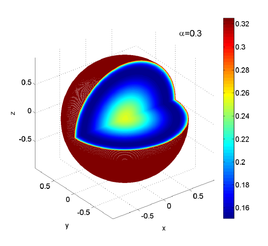
Figure 1: Density $H(\mathbf{x},t)$ of $3$-dimensional isotropic standard Lévy walk for $t=1$ and $\alpha=0.3$ obtained from Eqs. 3.1 and 23.

3.2 Even number of dimensions - $d=2n+2$

The calculations are getting more complicated when $d$ is even, however the idea remains the same. First we find the PDF $\Phi_{1}(x)$ of the first-coordinate process $X_{1}(1)$. The function $g_{1}(\xi)$ (Eq. (9)) now has the form

$$g_{1}(\xi)=\frac{\int_{-1}^{1}(1-\xi u)^{\alpha-1}\left(1-u^{2}\right)^{n-1/2}du}{\int_{-1}^{1}(1-\xi u)^{\alpha}\left(1-u^{2}\right)^{n-1/2}du}.$$ (24)

Using the hypergeometric functions the above equation can be rewritten:

$$g_{1}(\xi)=\frac{{}_{2}F_{1}((1-\alpha)/2,1-\alpha/2;1+n;\xi^{2})}{{}_{2}F_{1}(-\alpha/2,(1-\alpha)/2;1+n;\xi^{2})}.$$ (25)

Once again we apply the method of Godrèche and Luck to get

$$\Phi_{1}(x)=-\frac{1}{\pi\left|x\right|}\operatorname{Im}\frac{{}_{2}F_{1}((1-\alpha)/2,1-\alpha/2;1+n;\frac{1}{x^{2}})}{{}_{2}F_{1}(-\alpha/2,(1-\alpha)/2;1+n;\frac{1}{x^{2}})},\quad x\in(0,1).$$ (26)

The relation between $\Phi_{R}$ and $\Phi_{1}$ now has the form

$$\mathbf{P}(|X_{1}(1)|\leq x)=2c_{n}\int_{0}^{1}\mathbf{P}\left(\left\|\mathbf{X}(1)\right\|\leq\frac{x}{u}\right)\left(1-u^{2}\right)^{n-1/2}du,$$ (27)

where $c_{n}=\frac{1}{\sqrt{\pi}}\frac{\Gamma(n+1)}{\Gamma(n+1/2)}$ for $x\geq 0$. Following the reasoning we used for the odd number of dimensions we obtain

$$\Phi_{1}(\sqrt{x})=\frac{c_{n}\Gamma(n+1/2)}{2}I_{-}^{n+1/2}\{\Phi_{R}(\sqrt{u})u^{-n-1}\}(x)$$ (28)

and hence

$$\Phi_{R}(\sqrt{r})=\frac{2\sqrt{\pi}}{\Gamma(n+1)}r^{n+1/2}D_{-}^{n+1/2}\{\Phi_{1}(\sqrt{t})\}(r)$$ (29)

if $r\in(0,1)$ and $\Phi_{R}(r)=0$ otherwise. Here $D_{-}^{n+1/2}$ is the right-side Riemann-Liouville fractional derivative of order $n+1/2$ [34]:

$$D_{-}^{n+1/2}\{f(x)\}(y)=\left(-\frac{d}{dy}\right)^{n}\frac{1}{\pi^{1/2}}\int_{y}^{\infty}\frac{f(x)}{(x-y)^{1/2}}dx.$$ (30)

Fig. 2 presents the densities $\Phi_{R}$ for different number of dimensions $d$. For even $d$ it is necessary to numerically calculate the fractional derivative. This was done in Matlab using algorithm from [35]. In Cartesian coordinates $H(\mathbf{x},t)$ can be calculated as

$$H(\mathbf{x},t)=\frac{\Gamma(n+1)}{2\pi^{n+1}t\left\|\mathbf{x}\right\|^{2n+1}}\Phi_{R}\left(\frac{\left\|\mathbf{x}\right\|}{t}\right).$$ (31)

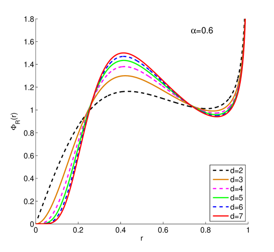
Figure 2: Densities $\Phi_{R}(r)$ of radii of $d$-dimensional isotropic standard Lévy walks for $\alpha=0.6$. Odd number of dimensions - Eq. 21 (elementary functions), even number - Eq. 29 and numerical scheme [35].

4 Undershooting and overshooting Lévy walks

The methods which we used to get the explicit densities of standard Lévy walks can be also applied for limits of under- and overshooting Lévy walks. Recall the notation $\mathbf{Y}(t)=(Y_{1}(t),Y_{2}(t),...,Y_{d}(t))$ for undershooting and $\mathbf{Z}(t)=(Z_{1}(t),Z_{2}(t),...,Z_{d}(t)$ for overshooting Lévy walk.

The relation between the PDF $\Phi_{1}^{Y}$ of $Y_{1}(1)$ and the PDF $\Phi_{R}^{Y}$ of $\left\|\mathbf{Y}(1)\right\|$ remains the same as for standard Lévy walks. Similarly for the PDF $\Phi_{1}^{Z}$ of $Z_{1}(1)$ and the PDF $\Phi_{R}^{Z}$ of $\left\|\mathbf{Z}(1)\right\|$. We only have to calculate $\Phi_{1}^{Y}$ and $\Phi_{1}^{Z}$.

4.1 Undershooting - odd number of dimensions $d=2n+3$

The PDF of $\mathbf{Y}(t)$ in Fourier-Laplace space is given by (see [31])

$$H(\mathbf{k},s)=\frac{1}{s}g\left(\frac{i\mathbf{k}}{s}\right)=\frac{1}{s}\frac{1}{\int_{\mathbf{S}^{d-1}}\left(1-\left\langle\frac{i\mathbf{k}}{s},\mathbf{u}\right\rangle\right)^{\alpha}K(d\mathbf{u})},$$

where $\mathbf{k}=(k_{1},k_{2},...,k_{d})\in\mathbb{R}^{d}$ is the Fourier space variable, $s$ is the Laplace space variable. The inversion formula yields

$$\begin{split}&\Phi^{Y}_{1}(x)=\frac{\sin(\pi\alpha)}{\sqrt{\pi}x^{2n+2}}\frac{\Gamma(n+1)}{\Gamma(n+3/2)}\mathcal{B}_{1}\cdot\bigg{\{}(-1)^{m}(1/x-1)^{m+j+\alpha+1}(1/x^{2}-1)^{n-m}\bigg{\}}\\ &/\mathcal{B}_{2}\cdot\bigg{\{}\left((-1)^{j_{1}+j_{2}}(1+1/x)^{m_{1}+m_{2}+j_{1}+j_{2}+2\alpha+2}+(-1)^{m_{1}+m_{2}}(1/x-1)^{m_{1}+m_{2}+j_{1}+j_{2}+2\alpha+2}\right.\\ &\left.+2\cos(\pi\alpha)(-1)^{j_{1}+m_{2}}(1/x+1)^{m_{1}+j_{1}+\alpha+1}(1/x-1)^{m_{2}+j_{2}+\alpha+1}\right)(1/x^{2}-1)^{2n-m_{1}-m_{2}}\bigg{\}},\end{split}$$ (32)

for $x\in(0,1)$, $\Phi^{Y}_{1}(-x)=\Phi^{Y}_{1}(x)$ for $x\in(-1,0)$ and $\Phi^{Y}_{1}(x)=0$ otherwise. The symbols $\mathcal{B}_{1}$ and $\mathcal{B}_{2}$ equal here

$$\mathcal{B}_{1}=\sum_{m}^{n}\sum_{j=0}^{m}{n\choose m}{m\choose j}2^{m-j}\frac{1}{m+j+\alpha+1},$$ (33)

$$\mathcal{B}_{2}=\sum_{m_{1},m_{2}=0}^{n}\sum_{j_{1}=0}^{m_{1}}\sum_{j_{2}=0}^{m_{2}}{n\choose m_{1}}{m_{1}\choose j_{1}}{n\choose m_{2}}{m_{2}\choose j_{2}}2^{m_{1}+m_{2}-j_{1}-j_{2}}\frac{1}{(m_{1}+j_{1}+\alpha+1)(m_{2}+j_{2}+\alpha+1)}.$$ (34)

One can also use special functions

$$\begin{split}\Phi^{Y}_{1}(x)=-\frac{1}{\pi\left|x\right|}\operatorname{Im}\frac{1}{{}_{2}F_{1}(-\alpha/2,(1-\alpha)/2;3+n/2;\frac{1}{x^{2}})}.\end{split}$$ (35)

The PDF $\Phi^{Y}_{R}$ is calculated from the equation

$$\Phi_{R}^{Y}(\sqrt{r})=\frac{2\sqrt{\pi}}{\Gamma(n+3/2)}r^{n+1}(-1)^{n+1}\frac{d^{n+1}}{dr^{n+1}}\Phi_{1}^{Y}(\sqrt{r})$$ (36)

if $r\in(0,1)$ and $\Phi^{Y}_{R}(r)=0$ otherwise. In the special case $d=3$ this gives us

$$\begin{split}&\Phi^{Y}_{R}(r)=\frac{4(\alpha+1)}{\pi}\sin(\pi\alpha)(1-r)^{\alpha}r^{-1+\alpha}\times\\ &\frac{(1-r)^{2+2\alpha}(1-\alpha-2r)+(1+r)^{1+2\alpha}(1-\alpha+3(1+\alpha)r-2r^{2})+2(1-\alpha+2r)(1-r^{2})^{2+\alpha}\cos(\alpha\pi)}{((1-r)^{2+2\alpha}+(1+r)^{2+2\alpha}+2(1-r^{2})^{1+\alpha}\cos(\alpha\pi))^{2}}\end{split}$$ (37)

for $r\in(0,1)$ and $\Phi^{Y}_{R}(r)=0$ for $r>1$. In Cartesian coordinates $H(\mathbf{x},t)$ can be calculated as

$$H(\mathbf{x},t)=\frac{\Gamma(n+3/2)}{2\pi^{n+3/2}t\left\|\mathbf{x}\right\|^{2n+2}}\Phi_{R}^{Y}\left(\frac{\left\|\mathbf{x}\right\|}{t}\right),$$ (38)

The density $H(\mathbf{x},t)$ is given by elementary functions for all $n$.

4.2 Overshooting - odd number of dimensions $d=2n+3$

For overshooting Lévy walk we get [31]

$$H(\mathbf{k},s)=\frac{1}{s}g\left(\frac{i\mathbf{k}}{s}\right)=\frac{1}{s}\left(1-\frac{c\left(\frac{i\mathbf{k}}{s}\right)^{\alpha}(\cos(\pi\alpha/2)-i\sin(\pi\alpha/2))}{\int_{\mathbf{S}^{d-1}}\left(1-\left\langle\frac{i\mathbf{k}}{s},\mathbf{u}\right\rangle\right)^{\alpha}K(d\mathbf{u})}\right),$$

where $c=\frac{\cos(\alpha\pi/2)\Gamma(2-\alpha)\Gamma((1+\alpha)/2)\Gamma(3/2+n)}{(1-\alpha)\sqrt{\pi}\Gamma(1-\alpha)\Gamma(3/2+\alpha/2+n)}$ The inversion formula implies

$$\begin{split}&\Phi^{Z}_{1}(x)=\frac{c\Gamma(n+1)}{\Gamma(n+3/2)\sqrt{\pi}x^{2n+2+\alpha}}\mathcal{B}_{1}\cdot\bigg{\{}(1/x^{2}-1)^{n-m}\big{[}-\cos(\pi\alpha/2)\sin(\pi\alpha)(-1)^{m}(1/x-1)^{m+j+\alpha+1}\\ &+\sin(\pi\alpha/2)\left((-1)^{j}(1/x+1)^{m+j+\alpha+1}+(-1)^{m}(1/x-1)^{m+j+\alpha+1}\sin(\pi\alpha/2)\cos(\pi\alpha)\right)\big{]}\bigg{\}}\\ &/\mathcal{B}_{2}\cdot\bigg{\{}\left((-1)^{j_{1}+j_{2}}(1+1/x)^{m_{1}+m_{2}+j_{1}+j_{2}+2\alpha+2}+(-1)^{m_{1}+m_{2}}(1/x-1)^{m_{1}+m_{2}+j_{1}+j_{2}+2\alpha+2}\right.\\ &\left.+2\cos(\pi\alpha)(-1)^{j_{1}+m_{2}}(1/x+1)^{m_{1}+j_{1}+\alpha+1}(1/x-1)^{m_{2}+j_{2}+\alpha+1}\right)(1/x^{2}-1)^{2n-m_{1}-m_{2}}\bigg{\}}\end{split}$$ (39)

for $x\in(0,1)$ and

$$\begin{split}&\Phi^{Z}_{1}(x)=\frac{c\Gamma(n+1)\sin(\pi\alpha/2)}{\Gamma(n+3/2)\sqrt{\pi}x^{2n+2+\alpha}}/\mathcal{B}_{1}\cdot\bigg{\{}(-1)^{j}\left((1+1/x)^{m+j+\alpha+1}-(1-1/x)^{m+j+\alpha+1}\right)(1/x^{2}-1)^{n-m}\}\end{split}$$ (40)

for $x\in[1,\infty)$. For negative values of $x$ we take advantage from the symmetry $\Phi^{Z}_{1}(-x)=\Phi^{Z}_{1}(x)$. The symbols $\mathcal{B}_{1}$ and $\mathcal{B}_{2}$ are given by

$$\mathcal{B}_{1}=\sum_{m}^{n}\sum_{j=0}^{m}{n\choose m}{m\choose j}2^{m-j}\frac{1}{m+j+\alpha+1},$$ (41)

$$\mathcal{B}_{2}=\sum_{m_{1},m_{2}=0}^{n}\sum_{j_{1}=0}^{m_{1}}\sum_{j_{2}=0}^{m_{2}}{n\choose m_{1}}{m_{1}\choose j_{1}}{n\choose m_{2}}{m_{2}\choose j_{2}}2^{m_{1}+m_{2}-j_{1}-j_{2}}\frac{1}{(m_{1}+j_{1}+\alpha+1)(m_{2}+j_{2}+\alpha+1)}.$$ (42)

Alternatively

$$\begin{split}\Phi^{Z}_{1}(x)=-\frac{c}{\pi\left|x\right|^{\alpha+1}}\operatorname{Im}\frac{\cos(\pi\alpha/2)+i\sin(\pi\alpha/2)}{{}_{2}F_{1}(-\alpha/2,(1-\alpha)/2;3/2+n;\frac{1}{x^{2}})}.\end{split}$$ (43)

The PDF $\Phi^{Z}_{R}$ is calculated from the equation

$$\Phi_{R}^{Z}(\sqrt{r})=\frac{2\sqrt{\pi}}{\Gamma(n+3/2)}r^{n+1}(-1)^{n+1}\frac{d^{n+1}}{dr^{n+1}}\Phi_{1}^{Z}(\sqrt{r})$$ (44)

if $r\in(0,\infty)$ and $\Phi^{Z}_{R}(r)=0$ otherwise. In a special case $d=3$ we obtain

$$\begin{split}\Phi^{Z}_{R}(r)=&\frac{2\sin(\pi\alpha)}{\pi r}\Bigg{(}(r+1)^{2\alpha+1}((\alpha+2)r^{2}-3(\alpha+1)r-1)(1-r)^{\alpha}\\ &\quad-2(1-r^{2})^{\alpha}(((\alpha+2)r+1)(1-r)^{\alpha+2}+(r+1)^{\alpha+2}((\alpha+2)r-1))\cos(\pi\alpha)\\ &\quad-(r+1)^{\alpha}(r(\alpha(r+3)+2r+3)-1)(1-r)^{2\alpha+1}\\ &\quad-(1-(\alpha+2)r)(1-r)^{3\alpha+2}-(r+1)^{3\alpha+2}((\alpha+2)r+1))\Bigg{)}/\\ &\quad\quad\quad\Bigg{(}(2(1-r^{2})^{\alpha+1}\cos(\pi\alpha)+(1-r)^{2\alpha+2)}+(r+1)^{2\alpha+2})^{2}\Bigg{)}\end{split}$$ (45)

for $r\in(0,1)$ and

$$\Phi^{Z}_{R}(r)=\frac{2\sin(\alpha\pi)}{\pi}\frac{(1+r)^{\alpha}(1+(2+\alpha)r)-(-1+r)^{\alpha}(-1+(2+\alpha)r)}{r((-1+r)^{1+\alpha}-(1+r)^{1+\alpha})^{2}}$$ (46)

for $r\in(1,\infty)$. In Cartesian coordinates this gives us

$$H(\mathbf{x},t)=\frac{\Gamma(n+3/2)}{2\pi^{n+3/2}t\left\|\mathbf{x}\right\|^{2n+2}}\Phi_{R}^{Z}\left(\frac{\left\|\mathbf{x}\right\|}{t}\right),$$ (47)

The density $H(\mathbf{x},t)$ is given by elementary functions for all $n$.

4.3 Undershooting - even number of dimensions $d=2n+2$

In this case

$$\begin{split}\Phi^{Y}_{1}(x)&=-\frac{1}{\pi\left|x\right|}\operatorname{Im}\frac{1}{{}_{2}F_{1}(-\alpha/2,(1-\alpha)/2;1+n;\frac{1}{x^{2}})}\end{split}$$ (48)

on the interval $(0,1)$. Moreover

$$\Phi_{R}^{Y}(\sqrt{r})=\frac{2\sqrt{\pi}}{\Gamma(n+1)}r^{n+1/2}D_{-}^{n+1/2}\{\Phi_{1}^{Y}(\sqrt{t})\}(r).$$ (49)

if $r\in(0,1)$ and $\Phi^{Y}_{R}(r)=0$ otherwise. Going back to Cartesian coordinates

$$H(\mathbf{x},t)=\frac{\Gamma(n+1)}{2\pi^{n+1}t\left\|\mathbf{x}\right\|^{2n+1}}\Phi_{R}^{Y}\left(\frac{\left\|\mathbf{x}\right\|}{t}\right).$$ (50)

4.4 Overshooting - even number of dimensions $d=2n+2$

Now we have

$$\begin{split}\Phi^{Z}_{1}(x)&=-\frac{c}{\pi\left|x\right|^{\alpha+1}}\operatorname{Im}\frac{\cos(\frac{1}{2}\pi\alpha)+i\sin(\frac{1}{2}\pi\alpha)}{{}_{2}F_{1}(-\alpha/2,(1-\alpha)/2;1+n;\frac{1}{x^{2}})}.\end{split}$$ (51)

In the above equation the constant $c$ is defined as $c=\frac{\cos(\alpha\pi/2)\Gamma(2-\alpha)\Gamma((1+\alpha)/2)\Gamma(1+n)}{(1-\alpha)\sqrt{\pi}\Gamma(1-\alpha)\Gamma(1+\alpha/2+n)}$. The density of the radius:

$$\Phi_{R}^{Z}(\sqrt{r})=\frac{2\sqrt{\pi}}{\Gamma(n+1)}r^{n+1/2}D_{-}^{n+1/2}\{\Phi_{1}^{Z}(\sqrt{t})\}(r).$$ (52)

if $r\in(0,\infty)$ and $\Phi^{Z}_{R}(r)=0$ otherwise. In Cartesian coordinates

$$H(\mathbf{x},t)=\frac{\Gamma(n+1)}{2\pi^{n+1}t\left\|\mathbf{x}\right\|^{2n+1}}\Phi_{R}^{Z}\left(\frac{\left\|\mathbf{x}\right\|}{t}\right).$$ (53)

Appendix A Inversion of F-L transform for 1D ballistic processes

In this appendix we present the method of inverting the Fourier-Laplace transform for 1D ballistic Lévy walks from [25] and [30]. The Fourier-Laplace transform of $H_{1}(x,t)$ is given by

$$H_{1}(k,s) =\int_{-\infty}^{\infty}\int_{0}^{\infty}e^{-ikx-st}H_{1}(x,t)dtdx$$ (55)

$$=\int_{-\infty}^{\infty}\int_{0}^{\infty}e^{-ikx-st}\frac{1}{t}\Phi_{1}\left(\frac{x}{t}\right)dtdx.$$

We substitute $y=\frac{x}{t}$ to get

$$H_{1}(k,s) =\int_{-\infty}^{\infty}\int_{0}^{\infty}e^{-(iky+s)t}\Phi_{1}\left(y\right)dtdy$$ (58)

$$=\int_{-\infty}^{\infty}\frac{1}{iky+s}\Phi_{1}\left(y\right)dy=\frac{1}{s}\int_{-\infty}^{\infty}\frac{1}{\frac{ik}{s}y+1}\Phi_{1}\left(y\right)dy$$

$$=\frac{1}{s}\mathbf{E}\frac{1}{\frac{ik}{s}X_{1}(1)+1}.$$

Hence

$$g_{1}(\xi)=\mathbf{E}\frac{1}{1+\xi X_{1}(1)}.$$ (59)

Now, the density $\Phi_{1}(x)$ can be written as

$$\Phi_{1}(x)=\mathbf{E}\delta(x-X_{1}(1)).$$ (60)

The Sokhotsky-Weierstrass theorem implies

$$\lim_{\varepsilon\rightarrow 0}\frac{1}{x\pm i\varepsilon}=\frac{1}{x}\mp i\pi\delta(x).$$ (61)

We infer that

$$\delta(x)=-\operatorname{Im}\lim_{\varepsilon\rightarrow 0}\frac{1}{x+i\varepsilon}.$$ (62)

Combining Eqs. (60) and (62) gives us

$$\Phi_{1}(x) =-\operatorname{Im}\lim_{\varepsilon\rightarrow 0}\mathbf{E}\frac{1}{x-X_{1}(1)+i\varepsilon}$$ (64)

$$=-\lim_{\varepsilon\rightarrow 0}\operatorname{Im}\frac{1}{x+i\varepsilon}\mathbf{E}\frac{1}{1-\frac{X_{1}(1)}{x+i\varepsilon}}$$

which yields

$$\Phi_{1}(x)=-\frac{1}{\pi}\lim_{\varepsilon\rightarrow 0}\operatorname{Im}\left[\frac{1}{x+i\varepsilon}\mathbf{E}\frac{1}{1-\frac{X_{1}(1)}{x+i\varepsilon}}\right].$$ (65)

Now we combine Eqs. (59) and (65) and get the formula for $\Phi_{1}$ (Eq. (11)). Notice that to formally get Eq. (11) we have to choose the Fourier space variable $k$ and Laplace space variable $s$ such that $\frac{ik}{s}=\frac{-1}{x+i\varepsilon}$. This is obtained by taking $s=s_{1}+is_{2}$ where $s_{1}=\varepsilon>0$, $s_{2}=-x$ and $k=1$. Since $s_{1}>0$ and $k\in\mathbb{R}$ the Fourier-Laplace transform is well defined and $H_{1}(k,s)=\frac{1}{s}g_{1}\left(\frac{ik}{s}\right)$ even for complex values of $s$ (providing that $s_{1}>0$).

References

- [1] M.F. Shlesinger, J. Klafter, and Y.M Wong, J. Stat. Phys. 27, 499 (1982).
- [2] J. Klafter, A. Blumen, and M.F. Shlesinger, Phys. Rev. A 35, 3081 (1987).
- [3] G. Ariel, A. Rabani, S. Benisty, J.D. Partridge, R.M. Harshey, and A. Be’er, Nature Communications 6, 8396 (2015).
- [4] G. Margolin and E. Barkai, Phys. Rev. Lett. 94, 080601 (2005).
- [5] P. Barthelemy, P.J. Bertolotti, and D.S. Wiersma, Nature 453, 495 (2008).
- [6] T.H. Solomon, E.R. Weeks, and H.L. Swinney, Phys. Rev. Lett. 71, 3975 (1993).
- [7] W.J. Bell, Searching Behaviour: The Behavioural Ecology of Finding Resources (Chapman and Hall, London, 1991).
- [8] H.C. Berg, Random Walks in Biology, Princeton University Press, Princeton, 1993.
- [9] M. Buchanan, Nature 453, 714 (2008).
- [10] D. Brockmann, L. Hufnagel, and T. Geisel, Nature 439, 462 (2006).
- [11] M.C. Gonzales, C.A. Hidalgo, A.L. Barabasi, Nature 453, 779 (2008).
- [12] D. Brockmann, V. David, and A.M. Gallardo, Rev. Nonlinear Dyn. Complex. 2, 1 (2009).
- [13] B. Dybiec, Phys. A 387, 4863 (2008).
- [14] V. Zaburdaev, S. Denisov, and J. Klafter, Lévy walks, Rev. Mod. Phys. 87, 483 (2015).
- [15] R. Metzler, and J. Klafter, Phys. Rep. 339, 1 (2000).
- [16] J. Klafter and I.M. Sokolov, First Steps in Random Walks. From Tools to Applications (Oxford University Press, Oxford, 2011).
- [17] A. Janicki and A. Weron, Simulation and Chaotic Behavior of -Stable Stochastic Processes (Dekker, New York, 1994).
- [18] A. Hanyga, Proc. R. Soc. Lond. A 457, 2993 (2001).
- [19] J. Li and M. Ostoja-Starzewski, Proc. R. Soc. A 465, 2521 (2009).
- [20] M.M Meerschaert and A. Sikorskii, Stochastic models for fractional calculus (De Gruyter, Berlin, 2012)
- [21] M. Magdziarz, W. Szczotka, P. Zebrowski, Proc. R. Soc. A 469, 20130419 (2013).
- [22] M. Magdziarz, H.P. Scheffler, P. Straka, and P. Zebrowski, Stoch. Proc. Appl. 125, 4021 (2015).
- [23] I.M. Sokolov and R. Metzler, Phys. Rev. E 67, 1 (2003).
- [24] V.V. Uchaikin and R.T. Sibatov, J. Phys. A: Math. Theor. 44, 145501 (2011).
- [25] D. Froemberg, M. Schmiedeberg, E. Barkai, and V. Zaburdaev, Phys. Rev. E 91, 022131 (2015).
- [26] M. Magdziarz, T. Zorawik, arXiv:1504.05835 (2015).
- [27] M. Magdziarz, T. Zorawik, arXiv:1510.05614 (2015).
- [28] V. Zaburdaev, I. Fouxon, S. Denisov, E. Barkai, arXiv:1605.02908 (2016).
- [29] V. V. Uchaikin and V. M. Zolotarev, Chance and Stability: Stable Distributions and their Applications (De Gruyter 1999).
- [30] C. Godrèche, J. M. Luck, J. Stat. Phys., 104, 3 (2001).
- [31] M. Magdziarz , M. Teuerle, Commun. Nonlinear Sci. Numer. Simul. 20, 489 (2015).
- [32] M. Teuerle, P. Zebrowski, M. Magdziarz, J. Phys. A: Math. Theor. 45 (2012).
- [33] M. Abramowitz and I.A. Stegun, Hypergeometric Functions. Ch. 15 in Handbook of Mathematical Functions with Formulas, Graphs, and Mathematical Tables (Dover, New York, 1972).
- [34] A.A. Kilbas, H.M. Srivastava, and J.J. Trujillo, Theory and Applications of Fractional Differential Equations (North - Holland Mathematics Studies, Amsterdam, 2006).
- [35] I. Podlubny, http://www.mathworks.com/matlabcentral/ fileexchange/22071