Expected values of parameters associated with the minimum rank of a graph

Abstract

We investigate the expected value of various graph parameters associated with the minimum rank of a graph, including minimum rank/maximum nullity and related Colin de Verdière-type parameters. Let $G(v,p)$ denote the usual Erdős-Rényi random graph on $v$ vertices with edge probability $p$. We obtain bounds for the expected value of the random variables $\operatorname{mr}(G(v,p))$, $\operatorname{M}(G(v,p))$, $\nu(G(v,p))$ and $\xi(G(v,p))$, which yield bounds on the average values of these parameters over all labeled graphs of order $v$.

AMS subject classifications: 05C50; 05C80; 15A03

Keywords: minimum rank; maximum nullity; average minimum rank; average maximum nullity; expected value; Colin de Verdière type parameter; positive semidefinite minimum rank; delta conjecture; rank; matrix; random graph; graph

1 Introduction

The set of $v\times v$ real symmetric matrices will be denoted by $\mathbb{R}^{(v)}$. For $A\in\mathbb{R}^{(v)}$, the graph of $A$, denoted $\mathcal{G}(A)$, is the graph with vertices $\{1,\dots,v\}$ and edges $\{\{i,j\}:~{}a_{ij}\neq 0,1\leq i<j\leq v\}$. Note that the diagonal of $A$ is ignored in determining $\mathcal{G}(A)$. The minimum rank of a graph $G$ on $v$ vertices is

$$\operatorname{mr}(G)=\min\{\operatorname{rank}A:A\in\mathbb{R}^{(v)},\mathcal{G}(A)=G\}.$$

The maximum nullity or maximum corank of a graph $G$ is

$$\operatorname{M}(G)=\max\{\operatorname{null}A:A\in\mathbb{R}^{(v)},\mathcal{G}(A)=G\}.$$

Note that

$$\operatorname{mr}(G)+\operatorname{M}(G)=v.$$

Here a graph is a pair $G=(V(G),E(G))$, where $V$ is the (finite, nonempty) set of vertices and $E$ is the set of edges (an edge is a two-element subset of vertices); what we call a graph is sometimes called a simple undirected graph. We use the notation $v(G)=|V(G)|$ and $e(G)=|E(G)|$.

The minimum rank problem (of a graph, over the real numbers) is to determine $\operatorname{mr}(G)$ for any graph $G$. See [12] for a survey of known results and discussion of the motivation for the minimum rank problem; an extensive bibliography is also provided there. The minimum rank problem was a focus of the 2006 workshop “Spectra of families of matrices described by graphs, digraphs, and sign patterns” held at the American Institute of Mathematics [2]. One of the questions raised during the workshop was:

Question 1.1.

What is the average minimum rank of a graph on $v$ vertices?

Formally, we define the average minimum rank of graphs of order $v$ to be the sum over all labeled graphs of order $v$ of the minimum ranks of the graphs, divided by the number of (labeled) graphs of order $v$. That is,

$$\operatorname{amr}(v)=\frac{\sum_{v(G)=v}\operatorname{mr}(G)}{2^{v\choose 2}}.$$

Let $G(v,p)$ denote the Erdős-Rényi random graph on $v$ vertices with edge probability $p$. That is, every pair of vertices is adjacent, independently, with probability $p$. Note that for $G(v,1/2)$, every labeled $v$-vertex graph is equally likely (each labeled graph is chosen with probability $2^{-\binom{v}{2}}$), so

$$\operatorname{amr}(v)=E\left[\operatorname{mr}(G(v,1/2))\right].$$

Our goal in this paper is to determine statistics about the random variable $\operatorname{mr}(G(v,p))$ and other related parameters. We highlight the two main results of this paper by focusing on the $p=1/2$ case:

Theorem 1.2.

Given $\operatorname{amr}(v)=E\left[\operatorname{mr}(G(v,1/2))\right]$, then for $v$ sufficiently large,

1. $\displaystyle\left|\operatorname{mr}(G(v,1/2))-\operatorname{amr}(v)\right|<\sqrt{v\ln\ln v}$ with probability approaching 1 as $v\rightarrow\infty$, and

2. $0.146907v<\operatorname{amr}(v)<0.5v+\sqrt{7v\ln v}$.

In general, we show that the random variable $\operatorname{mr}(G(v,p))$ is tightly concentrated around its mean (Section 2), and establish lower and upper bounds for its expected value in Sections 4 and 5. We also establish an upper bound on the Colin de Verdière type parameter $\xi(G)$, which is related to $\operatorname{M}(G)$, in Section 6 (the definition of $\xi$ is given in that section). This bound is used in Section 7 to establish bounds on the expected value of the random variable $\xi(G(v,p))$. The upper bound on $\xi(G(v,p))$ may lead to a better upper bound on the expected value of $\operatorname{M}(G(v,p))$ and hence a better lower bound on the expected value of $\operatorname{mr}(G(v,p))$.

2 Tight concentration of expected minimum rank

Although we are unable to determine precisely the mean of $\operatorname{mr}(G(v,p))$, in this section we show that this random variable is tightly concentrated around its mean, and thus $\operatorname{mr}(G(v,1/2))$ is tightly concentrated around the average minimum rank.

A martingale is a sequence of random variables $X_{0},\dots,X_{v-1}$ such that

$${\bf E}[X_{i+1}|X_{i},X_{i-1},\dots,X_{1}]=X_{i}.$$

The martingale we use is the vertex exposure martingale (as described on pages 94-95 of [1]) for the graph parameter $f(G)=\frac{1}{2}\operatorname{mr}(G)$ (the factor $\frac{1}{2}$ is needed because deletion of a vertex may change the minimum rank by $2$; see Corollary 2.3 below). $G(v,p)$ is sampled to obtain a specific graph $H$, and $X_{i}$ is the expected value of the graph parameter $f(G)=\frac{1}{2}\operatorname{mr}(G)$ when the neighbors of vertices $v_{1},\dots,v_{i}$ are known. Since nothing is known for $X_{0}$, $X_{0}={\bf E}[f(G(v,p))]=\frac{1}{2}{\bf E}[\operatorname{mr}(G(v,p))]$. Since the entire graph $H$ is revealed at stage $v-1$, $X_{v-1}=\frac{1}{2}\operatorname{mr}(H)$.

The method for showing tight concentration uses Azuma’s inequality for martingales (see Section 7.2 of [1]) and was pioneered by Shamir and Spencer [19]. The following corollary of Azuma’s inequality is used.

Theorem 2.1.

[1, Corollary 7.2.2] Let $b=X_{0},\dots,X_{v}$ be a martingale with

$$|X_{i+1}-X_{i}|\leq 1$$

for all $0\leq i\leq v$. Then

$$\Pr[|X_{v}-b|>\beta\sqrt{v}]<2e^{-\beta^{2}/2}.$$

The proof that derives the tight concentration of the chromatic number of the random graph [1, Theorem 7.2.4] from [1, Corollary 7.2.2] via the vertex exposure martingale remains valid for any graph parameter $f(G)$ such that when $G$ and $H$ differ only in the exposure of a single vertex, then $|f(G)-f(H)|\leq 1$.

Theorem 2.2.

Let $p\in(0,1)$. Let $f$ be a graph invariant such that for any graphs $G$ and $H$, if $x\in V(G)=V(H)$ and $G-x=H-x$, then $|f(G)-f(H)|\leq 1$. Let $\mu={\bf E}\left[f(G(v,p))\right]$. Then, for any $\beta>0$,

$$\Pr\left[\left|f(G(v,p))-\mu\right|>\beta\sqrt{v-1}\right]<2e^{-\beta^{2}/2}.$$

Corollary 2.3.

Let $p\in(0,1)$ be fixed and let $\mu={\bf E}\left[\operatorname{mr}(G(v,p))\right]$. For any $\beta>0$,

$$\Pr\left[\left|\operatorname{mr}(G(v,p))-\mu\right|>2\beta\sqrt{v-1}\right]<2e^{-\beta^{2}/2}.$$

In particular,

$$\left|\operatorname{mr}(G(v,p))-\mu\right|<\sqrt{v\ln\ln v}$$

with probability approaching $1$ as $v\rightarrow\infty$.

Proof.

It is well-known that for any graph $G$ and any vertex $x\in V(G)$, $0\leq\operatorname{mr}(G)-\operatorname{mr}(G-x)\leq 2.$ Thus if $V(H)=V(G)$ and $G-x=H-x$, then $|\operatorname{mr}(G)-\operatorname{mr}(H)|\leq 2$. For the first statement, apply Theorem 2.2 with $f(G)=\frac{1}{2}\operatorname{mr}(G)$. For the second statement, let $\beta=\frac{1}{2}\sqrt{\ln\ln v}$ and conclude

$$\Pr\left[\left|\operatorname{mr}(G(v,p))-\mu\right|>\sqrt{v\ln\ln v}\right]<2\left(\frac{1}{{\ln v}}\right)^{1/8}.$$

∎

Note that Corollary 2.3 gives the result in Theorem 1.2(1).

3 Observations on parameters of random graphs

Large deviation bounds easily show that the degree sequence of the random graph is tightly concentrated. In this section, we provide some well-known results that will be used later. The version of the Chernoff-Hoeffding bound that we use is given in [1].

Theorem 3.1.

[1, Theorem A.1.16] Let $X_{i}$, $1\leq i\leq n$, be mutually independent random variables with all ${\bf E}[X_{i}]=0$ and all $|X_{i}|\leq 1$. Set $S=X_{1}+\cdots+X_{n}$. Then for any $a>0$,

$$\Pr[S>a]<\exp\{-a^{2}/(2n)\}.$$

It is well-known that Theorem 3.1 can be applied to the number of edges in a random graph:

Theorem 3.2.

Let $p$ be fixed and let $G$ be distributed according to $G(v,p)$. Then,

$$e(G)\leq p\binom{v}{2}+v\sqrt{2\ln v},$$

with probability at least $1-v^{-2}$. In addition, $e(G)\geq p\binom{v}{2}-v\sqrt{2\ln v}$ with probability at least $1-v^{-2}$.

Proof.

Let $G$ be distributed according to the random variable $G(v,p)$. We may regard
$\left\{\{x,y\}\in E(G):x\neq y\right\}$ to be $\binom{v}{2}$ mutually independent indicator random variables. Subtract $p$ from each and they become random variables with mean $0$ and magnitude at most 1. Using Theorem 3.1, we see that $\Pr\left[e(G)-p\binom{v}{2}>a\right]<\exp\left\{-a^{2}/\left(2\binom{v}{2}\right)\right\}$.

Choose $a=v\sqrt{2\ln v}$; we see that

$$e(G)-p\binom{v}{2}\leq v\sqrt{2\ln v},$$

with probability at least $1-v^{-2}$. By multiplying the random variables above by $-1$, we obtain

$$e(G)-p\binom{v}{2}\geq-v\sqrt{2\ln v},$$

with probability at least $1-v^{-2}$. ∎

Let $\delta(G)$ (respectively, $\Delta(G)$) denote the minimum (maximum) degree of a vertex of $G$. Theorem 3.1 can also be applied to the neighborhood of each vertex to give bounds on $\delta(G)$ and $\Delta(G)$.

Theorem 3.3.

Let $p$ be fixed and let $G$ be distributed according to $G(v,p)$. Then,

$$pv-\sqrt{6v\ln v}\leq\delta(G)\leq\Delta(G)\leq pv+\sqrt{6v\ln v}$$

with probability at least $1-2v^{-2}$.

Proof.

Let $G$ be distributed according to the random variable $G(v,p)$. For each $x\in V(G)$, we may regard $\left\{\{x,y\}\in E(G):y\neq x\right\}$ to be $v-1$ mutually independent indicator random variables. Using Theorem 3.1, we see that $\Pr\left[\left|\deg(x)-p(v-1)\right|>a\right]<2\exp\{-a^{2}/(2(v-1))\}$.

Thus, the probability that there exists a vertex with degree that deviates by more than $a$ from $p(v-1)$ is at most

$$v\times 2\exp\{-a^{2}/(2(v-1))\}.$$

Choose $a=\sqrt{6v\ln v}$ and we see that, simultaneously for all $x\in V(G)$,

$$\left|\deg(x)-pv\right|\leq\sqrt{6v\ln v},$$

with probability at least $1-2v^{-2}$. ∎

4 A lower bound for expected minimum rank

In this section we show that if $v$ is sufficiently large, then the expected value of $\operatorname{mr}(G(v,p))$ is at least $c(p)v+o(v)$, where $c(p)$ is the solution to equation (1) below. In the case $p=1/2$, $c(p)\approx 0.1469077$, so the average minimum rank is greater than $0.146907v$ for $v$ sufficiently large.

The zero-pattern $\zeta({\bf x})$ of the real vector ${\bf x}=(x_{1},\ldots,x_{\ell})$ is the $(0,*)$-vector obtained from ${\bf x}$ by replacing its nonzero entries by $*$. The support of the zero pattern ${\bf z}=(z_{1},\dots,z_{\ell})$ is the set $S({\bf z})=\{i:z_{i}\neq 0\}$. We modify the proof of Theorem 4.1 from [18] to obtain the following result.

Theorem 4.1.

If ${\bf f}({\bf x})=(f_{1}({\bf x}),f_{2}({\bf x}),\ldots,f_{m}({\bf x}))$ is an $m$-tuple of polynomials in $n$ variables over a field $F$ with $m\geq n$, each $f_{i}$ of degree at most $d$, then the number of zero-patterns ${\bf z}=\zeta({\bf f}({\bf x}))$ with $|S({\bf z})|\leq s$ is at most

$${n+sd\choose n}.$$

Proof.

We follow the proof in [18]. Assume that the $m$-tuple ${\bf f}=(f_{1},\ldots,f_{m})$ of polynomials over field $F$ has the $M$ zero-patterns ${\bf z}_{1},\dots,{\bf z}_{M}$. Choose ${\bf u}_{1},\ldots,{\bf u}_{M}\in F^{n}$ such that $\zeta({\bf f}({\bf u}_{i}))={\bf z}_{i}$.

Set

$$g_{i}=\prod_{k\in S({\bf z}_{i})}f_{k}.$$

Note that

$$g_{i}({\bf u}_{j})\neq 0\qquad\mbox{if and only if}\qquad S({\bf z}_{i})\subseteq S({\bf z}_{j}).$$

We show that polynomials $g_{1},\ldots,g_{M}$ are linearly independent. Assume on the contrary that there is a nontrivial linear combination $\sum_{i=1}^{M}\beta_{i}g_{i}=0$, where each $\beta_{i}\in F$. Let $j$ be a subscript such that $|S({\bf z}_{j})|$ is minimal among the $S({\bf z}_{i})$ with $\beta_{i}\neq 0$, so for every $i$ such that $i\neq j$ and $\beta_{i}\neq 0$, $S({\bf z}_{i})\not\subseteq S({\bf z}_{j})$. So substituting ${\bf u}_{j}$ into the linear combination gives $\beta_{j}g_{j}({\bf u}_{j})=0$, a contradiction.

Thus, $g_{1},\ldots,g_{M}$ are linearly independent over $F$. Each $g_{i}$ has degree at most $sd$ and the dimension of the space of polynomials of degree $\leq D$ is exactly $\binom{n+D}{n}$. ∎

By Sylvester’s Law of Inertia, every real symmetric $v\times v$ matrix of rank at most $r$ can be expressed in the form $X^{T}D_{i}X$ for some $i$ such that $0\leq i\leq r$, where $D_{i}={\rm diag}(1,\dots,1,-1,\dots,-1)$ is an $r\times r$ diagonal matrix with $i$ diagonal entries equal to $1$ and $r-i$ equal to $-1$ and $X$ is an $r\times v$ real matrix. There are $r+1$ diagonal matrices $D_{i}$. Let each entry of $X$ be a variable; the total number of variables is $rv$ and each entry of the matrix $X^{T}D_{i}X$ is a polynomial of degree at most $2$.

Let $c(p)$ be the solution to

$$\frac{(c+p)^{2c+2p}}{(c)^{2c}(p)^{2p}}p^{p}(1-p)^{(1-p)}=1$$ (1)

for a fixed value of $p(0<p<1)$. This equation has a unique solution, because it is equivalent to $\frac{(c+p)^{2c+2p}}{c^{2c}}=\frac{p^{p}}{(1-p)^{(1-p)}}$, and for a fixed $p$ and $c\geq 0$, $\frac{(c+p)^{2c+2p}}{c^{2c}}$ is a strictly increasing function of $c$ and $p^{2p}<\frac{p^{p}}{(1-p)^{(1-p)}}$. The values of $c(p),0<p<1$ are graphed in Figure 1.

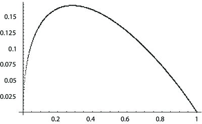
Figure 1: The graph of $c(p)$

Theorem 4.2.

Let $G$ be distributed according to $G(v,p)$ for a fixed $p$, $0<p<1$. For any $c<c(p)$, the expectation ${\bf E}\left[\operatorname{mr}(G)\right]$ satisfies

$${\bf E}\left[\operatorname{mr}(G)\right]>cv$$

for $v$ sufficiently large.

Furthermore, for any such $c$, $\Pr\left[\operatorname{mr}(G(v,p))\leq cv\right]\to 0$ as $v\to\infty$.

Proof.

Let $G$ be distributed according to $G(v,p)$. Let $\mathcal{E}$ be the event that $\left|e(G)-p\binom{v}{2}\right|\leq v\sqrt{2\ln v}$. By the law of total expectation,

$${\bf E}[\operatorname{mr}(G)] = {\bf E}[\operatorname{mr}(G)\mid{\mathcal{E}}]\Pr[{\mathcal{E}}]+{\bf E}[\operatorname{mr}(G)\mid{\mathcal{E}}^{c}]\Pr[{\mathcal{E}}^{c}]$$

$$\geq {\bf E}[\operatorname{mr}(G)\mid{\mathcal{E}}]\Pr\left[{\mathcal{E}}\right]$$

$$\geq (r+1)\Pr[\operatorname{mr}(G)>r\mid{\mathcal{E}}]\Pr[{\mathcal{E}}]$$

$$= (r+1)\left(1-\Pr[\operatorname{mr}(G)\leq r\mid{\mathcal{E}}]\right)\left(1-\Pr[{\mathcal{E}^{c}}]\right)$$

$$\geq (r+1)-(r+1)\Pr[\operatorname{mr}(G)\leq r\mid{\mathcal{E}}]-(r+1)\Pr[{\mathcal{E}}^{c}]$$

$$\geq (r+1)-v\Pr[\operatorname{mr}(G)\leq r\mid{\mathcal{E}}]-v\Pr[{\mathcal{E}}^{c}]$$

Theorem 3.2 shows that $v\Pr[{\mathcal{E}}^{c}]\leq v^{-1}$. It remains to bound $\Pr[\operatorname{mr}(G)\leq r\mid{\mathcal{E}}]$.

$$\Pr\left[\operatorname{mr}(G)\leq r\mid{\mathcal{E}}\right] = \sum_{\scriptsize\begin{array}[]{l}G:v(G)=v,\operatorname{mr}(G)\leq r\\ \left|e(G)-p\binom{v}{2}\right|\leq v\sqrt{2\ln v}\end{array}}\Pr[G\in G(v,p)]$$

$$= \sum_{\scriptsize\begin{array}[]{l}G:v(G)=v,\operatorname{mr}(G)\leq r\\ \left|e(G)-p\binom{v}{2}\right|\leq v\sqrt{2\ln v}\end{array}}p^{e(G)}(1-p)^{\binom{v}{2}-e(G)}$$

$$= \sum_{\scriptsize\begin{array}[]{l}G:v(G)=v,\operatorname{mr}(G)\leq r\\ \left|e(G)-p\binom{v}{2}\right|\leq v\sqrt{2\ln v}\end{array}}\left(\frac{p}{1-p}\right)^{e(G)}(1-p)^{\binom{v}{2}}$$

If $p<1/2$, then we use a lower bound for $e(G)$, given $\mathcal{E}$; if $p>1/2$, an upper bound. So, we can bound the term inside the summation as

$$\left(\frac{p}{1-p}\right)^{e(G)}(1-p)^{\binom{v}{2}}\leq\left(\frac{\max\{p,1-p\}}{\min\{p,1-p\}}\right)^{v\sqrt{2\ln v}}\left(p^{p}(1-p)^{(1-p)}\right)^{\binom{v}{2}}.$$

Hence,

$$\Pr\left[\operatorname{mr}(G)\leq r\mid{\mathcal{E}}\right]$$

$$\leq \left(\frac{\max\{p,1-p\}}{\min\{p,1-p\}}\right)^{v\sqrt{2\ln v}}\left(p^{p}(1-p)^{(1-p)}\right)^{\binom{v}{2}}\left|\left\{G:v(G)=v,\left|e(G)-p\binom{v}{2}\right|\leq v\sqrt{2\ln v},\operatorname{mr}(G)\leq r\right\}\right|.$$

The number of $v$ vertex graphs with between $p\binom{v}{2}-v\sqrt{2\ln v}$ and $p\binom{v}{2}+v\sqrt{2\ln v}$ edges and minimum rank at most $r$ is at most the number of $v\times v$ symmetric pattern matrices obtained as $X^{T}D_{i}X,i=0,\dots,r$ with $X$ an $r\times v$ matrix for which the cardinality of the support of the superdiagonal entries is at most $p\binom{v}{2}+v\sqrt{2\ln v}$. We can apply Theorem 4.1 with $n=rv$, $d=2$ and $s\leq p\binom{v}{2}+v\sqrt{2\ln v}$. Therefore, because there are $r+1$ diagonal matrices,

$$\Pr\left[\operatorname{mr}(G)\leq r\mid{\mathcal{E}}\right]$$

$$\leq \left(\frac{\max\{p,1-p\}}{\min\{p,1-p\}}\right)^{v\sqrt{2\ln v}}\left(p^{p}(1-p)^{(1-p)}\right)^{\binom{v}{2}}(r+1)\binom{rv+2p\binom{v}{2}+2v\sqrt{2\ln v}}{rv}.$$

By Corollary A.2 in Appendix A, for fixed $c$ and $p$ with $r=cv$,

$$\binom{rv+2p\binom{v}{2}+2v\sqrt{2\ln v}}{rv}\leq\left((1+o(1))\left(\frac{(c+p)^{c+p}}{c^{c}p^{p}}\right)\right)^{v^{2}}.$$

Thus

$$\Pr[\operatorname{mr}(G)\leq cv\mid{\mathcal{E}}]\leq\left((1+o(1))\frac{(c+p)^{2c+2p}}{(c)^{2c}(p)^{2p}}p^{p}(1-p)^{(1-p)}\right)^{v^{2}/2}.$$

As long $c<c(p)$ and $v$ is sufficiently large, the quantity $v\Pr\left[\operatorname{mr}(G)\leq r\mid{\mathcal{E}}\right]$ is less than 1, giving

$${\bf E}[\operatorname{mr}(G)]\geq(r+1)-v\Pr[\operatorname{mr}(G)\leq r\mid{\mathcal{E}}]-v\Pr[{\mathcal{E}}^{c}]>r+1-o(1)\geq r.$$

Furthermore, as long as $c<c(p)$, $\Pr\left[\operatorname{mr}(G)\leq cv\mid{\mathcal{E}}\right]\to 0$ as $v\to\infty$, and by Theorem 4.1, $\Pr[{\mathcal{E}}^{c}]\to 0$ as $v\to\infty$. Since

$$\Pr[\operatorname{mr}(G)\leq cv]\leq\Pr[\operatorname{mr}(G)\leq cv\mid{\mathcal{E}}]+\Pr[{\mathcal{E}}^{c}],$$

$\Pr[\operatorname{mr}(G)\leq cv]\to 0$ as $v\to\infty$. ∎

Corollary 4.3.

For $v$ sufficiently large, the average minimum rank over all labeled graphs of order $v$ satisfies

$$\operatorname{amr}(v)>0.146907v.$$

Furthermore, if $G$ is chosen at random from all labeled graphs of order $v$, $\Pr[\operatorname{mr}(G)\leq 0.146907v]\to 0$ as $v\to\infty$.

Proof.

For $p=1/2$, ${\bf E}[\operatorname{mr}(G)]=\operatorname{amr}(v)$ and $0.146907<c(p)$. ∎

Note that Corollary 2.3 gives the lower bound in Theorem 1.2(2). We note further the lack of symmetry with respect to $p$. The value $c(p)$ approaches zero as $p$ approaches zero, which is not the case with the upper bound that we describe in the next section.

5 An upper bound for expected minimum rank

In this section we show that if $v$ is sufficiently large, then the expected value of $\operatorname{mr}(G(v,p))$ is at most $(1-p)v+\sqrt{7v\ln v}$. Thus the average minimum rank for graphs of order $v$ is at most $0.5v+\sqrt{7v\ln v}$.

Let $\kappa(G)$ denote the vertex connectivity of $G$. That is, if $G$ is not complete, it is the smallest number $k$ such that there is a set of vertices $S$, with $|S|=k$, for which $G-S$ is disconnected. By convention, $\kappa(K_{v})=v-1$.

Following the terminology of [15], for a graph $G$ an orthogonal representation of $G$ of dimension $d$ is a set of vectors in $\mathbb{R}^{d}$, one corresponding to each vertex, such that if two vertices are nonadjacent, then their corresponding vectors are orthogonal. Every graph has an orthogonal representation in any dimension by associating the zero vector with every vertex. A faithful orthogonal representation of $G$ of dimension $d$ is a set of vectors in $\mathbb{R}^{d}$, one corresponding to each vertex, such that two (distinct) vertices are nonadjacent if and only if their corresponding vectors are orthogonal. Note that in the minimum rank literature, the term “orthogonal representation” is customarily used for what is here called a faithful orthogonal representation.

The following result of Lovász, Saks and Schrijver [15] (see also the note on errata, [16] Theorem 1.1) is the basis for an upper bound for minimum rank.

Theorem 5.1.

[15, Corollary 1.4] Every graph $G$ on $v$ vertices has a faithful orthogonal representation of dimension $v-\kappa(G)$.

Let $\operatorname{mr}_{+}(G)$ denote the minimum rank among all symmetric positive semidefinite matrices $A$ such that $\mathcal{G}(A)=G$, and let $\operatorname{M}_{+}(G)$ denote the maximum nullity among all such matrices. It is well known (and easy to see) that every faithful orthogonal representation of dimension $d$ gives rise to a positive semidefinite matrix of rank $d$ and vice versa.

Corollary 5.2.

For any graph $G$ on $v$ vertices,

$$\operatorname{mr}(G)\leq\operatorname{mr}_{+}(G)\leq v-\kappa(G),$$ (5)

or equivalently,

$$\kappa(G)\leq\operatorname{M}_{+}(G)\leq\operatorname{M}(G).$$ (6)

Our proof of the upper bound on the expected value of $\operatorname{mr}(G(v,p))$ uses the bound (5) and the relationship (on average) between the connectivity $\kappa(G)$ and the minimum degree $\delta(G)$. At the AIM workshop [2] it was conjectured that for any graph $G$, $\delta(G)\leq M(G)$, or equivalently $\operatorname{mr}(G)\leq v(G)-\delta(G)$ [9]. The conjecture was proved for bipartite graphs in [4] but remains open in general. In [15] it is reported that in 1987, Maehara made a conjecture equivalent to $\operatorname{mr}_{+}(G)\leq v(G)-\delta(G)$, which would imply $\operatorname{mr}(G)\leq v(G)-\delta(G)$.

Theorem 5.3.

Let $G$ be distributed according to $G(v,p)$. For $v$ sufficiently large, the expected value of minimum rank satisfies ${\bf E}[\operatorname{mr}(G)]\leq(1-p)v+\sqrt{7v\ln v}$.

For $v$ sufficiently large, the average minimum rank over all labeled graphs of order $v$ satisfies

$$\operatorname{amr}(v)\leq 0.5v+\sqrt{7v\ln v}.$$

Proof.

In [8] (see also section 7.2 of [7]), Bollobás and Thomason prove that if $G$ is distributed according to $G(v,p)$, then $\Pr[\kappa(G)=\delta(G)]\rightarrow 1$ as $v\rightarrow\infty$, without any restriction on $p$. Lemma B.1 in Appendix B shows that for $p$ fixed and $v$ large enough, $\Pr[\kappa(G)<\delta(G)]\leq 3v^{-2}$. Let $\mathcal{E}$ be the event that $\kappa(G)=\delta(G)$ and $\delta(G)\geq pv-\sqrt{6v\ln v}$. For $G$ distributed according to $G(v,p)$, the law of total expectation gives

$${\bf E}[\kappa(G)] = {\bf E}[\kappa(G)\mid{\mathcal{E}}]\Pr[{\mathcal{E}}]+{\bf E}[\kappa(G)\mid{\mathcal{E}}^{c}]\Pr[{\mathcal{E}}^{c}]$$

$$\geq \left(pv-\sqrt{6v\ln v}\right)\left(1-\Pr[{\mathcal{E}}^{c}]\right)$$

$$\geq pv-\sqrt{6v\ln v}-v\left(\Pr[\delta(G)<pv-\sqrt{6v\ln v}]+\Pr[\kappa(G)<\delta(G)]\right).$$

We use Theorem 3.3 and the result that $v\Pr[\kappa(G)<\delta(G)]\leq 3v^{-1}$ to see that

$${\bf E}\left[\kappa(G)\right]\geq pv-\sqrt{6v\ln v}-2v^{-1}-3v^{-1}\geq pv-\sqrt{7v\ln v},$$

for $v$ sufficiently large. By (5), ${\bf E}[\operatorname{mr}(G)]\leq(1-p)v+\sqrt{7v\ln v}$. ∎

Theorem 5.3 gives the upper bound in Theorem 1.2(2). Note that Theorem 5.3 actually establishes ${\bf E}[\operatorname{mr}_{+}(G)]\leq(1-p)v+\sqrt{7v\ln v}$. Since $\operatorname{mr}(G)\leq\operatorname{mr}_{+}(G)$ for any graph $G$, the lower bound in Theorem 4.2 in Section 4 certainly bounds ${\bf E}[\operatorname{mr}_{+}(G)]$ from below.

6 Bounds for $\nu(G)$ and $\xi(G)$

In this section we discuss the the Colin de Verdière type parameters $\nu(G)$ and $\xi(G)$, and establish an upper bound on $\xi(G)$ in terms of the number of edges of the graph. This upper bound, and a known lower bound for $\nu(G)$, have implications for the average value of $\nu$ and $\xi$ (see Section 7).

In 1990 Colin de Verdière ([10] in English) introduced the graph parameter $\mu$ that is equal to the maximum multiplicity of eigenvalue 0 among all matrices satisfying several conditions including the Strong Arnold Hypothesis (defined below). The parameter $\mu$, which is used to characterize planarity, is the first of several parameters that require the Strong Arnold Hypothesis and bound the maximum nullity from below (called Colin de Verdière type parameters). All the Colin de Verdière type parameters we discuss have been shown to be minor monotone.

A contraction of $G$ is obtained by identifying two adjacent vertices of $G$, deleting any loops that arise in this process, and replacing any multiple edges by a single edge. A minor of $G$ arises by performing a sequence of deletions of edges, deletions of isolated vertices, and/or contractions of edges. A graph parameter $\beta$ is minor monotone if for any minor $G^{\prime}$ of $G$, $\beta(G^{\prime})\leq\beta(G)$.

A symmetric real matrix $M$ is said to satisfy the Strong Arnold Hypothesis (SAH) provided there does not exist a nonzero real symmetric matrix $X$ satisfying $AX=0$, $A\circ X=0$, and $I\circ X=0$, where $\circ$ denotes the Hadamard (entrywise) product and $I$ is the identity matrix.

The SAH is equivalent to the requirement that certain manifolds intersect transversally. Specifically, for $A=[a_{ij}]\in\mathbb{R}^{(v)}$ let

$$\mathcal{R}_{A}=\{B\in\mathbb{R}^{(v)}:\operatorname{rank}B=\operatorname{rank}A\},$$

and

$$\mathcal{S}_{A}=\{B\in\mathbb{R}^{(v)}:\mathcal{G}(B)=\mathcal{G}(A)\}.$$

Then $\mathcal{R}_{A}$ and $\mathcal{S}_{A}$ intersect transversally at $A$ if and only if $A$ satisfies the SAH (see [14]).

Another minor monotone parameter, introduced by Colin de Verdière in [11], is denoted by $\nu(G)$ and defined to be the maximum nullity among matrices $A$ that satisfy:

1. $\mathcal{G}(A)=G$;

2. $A$ is positive semidefinite;

3. $A$ satisfies the Strong Arnold Hypothesis.

Clearly $\nu(G)\leq\operatorname{M}_{+}(G)$.

The parameter $\xi(G)$ was introduced in [3] as a Colin de Verdière type parameter intended for use in computing maximum nullity and minimum rank, by removing any unnecessary restrictions while preserving minor monotonicity. Define $\xi(G)$ to be the maximum multiplicity of 0 as an eigenvalue among matrices $A\in\mathbb{R}^{(v)}$ that satisfy:

• $\mathcal{G}(A)=G$.

• $A$ satisfies the Strong Arnold Hypothesis.

Clearly, $\nu(G)\leq\xi(G)\leq\operatorname{M}(G)$. The following lower bound on $\nu(G)$ has been established by van der Holst using the results of Lovász, Saks and Schrijver.

Theorem 6.1.

[13, Theorem 4] For every graph $G$,

$$\kappa(G)\leq\nu(G)\leq\xi(G).$$

The following bound on the Colin de Verdière number $\mu$ in terms of the number of edges $e(G)$ is given in [17] for any connected graph $G\neq K_{3,3}:$

$$e(G)\geq\frac{\mu(G)(\mu(G)+1)}{2}.$$

We will show that for any connected graph $G$,

$$e(G)+b\geq\frac{\xi(G)(\xi(G)+1)}{2}$$

where $b=1$ if $G$ is bipartite and $b=0$ otherwise.

For a manifold $\mathcal{M}$ and matrix $A\in\mathcal{M}$, let $\mathcal{T}_{\mathcal{M}_{A}}$ be the tangent space in $\mathbb{R}^{(v)}$ to $\mathcal{M}$ at $A$ and let $\mathcal{N}_{\mathcal{M}_{A}}$ be the normal (orthogonal complement) to $\mathcal{T}_{\mathcal{M}_{A}}$.

Observation 6.2.

[14, p. 9]

1. $\mathcal{T}_{\mathcal{S}_{A}}=\{B:\forall i\neq j,a_{ij}=0\Rightarrow b_{ij}=0\}$.

2. $\mathcal{N}_{\mathcal{S}_{A}}=\{X:\forall i,x_{ii}=0\mbox{ and }\forall i\neq j,a_{ij}\neq 0\Rightarrow x_{ij}=0\}$.

3. $\mathcal{T}_{\mathcal{R}_{A}}=\{WA+AW^{T}:W\in\mathbb{R}^{n\times n}\}=\{B\in\mathbb{R}^{(v)}:{\bf v}^{T}B{\bf v}=0~{}\forall{\bf v}\in\ker A\}$.

4. $\mathcal{N}_{\mathcal{R}_{A}}=\operatorname{span}(\{{\bf v}{\bf v}^{T}:{\bf v}\in\ker A\})=\{X\in\mathbb{R}^{(v)}:AX=0\}$.

Clearly $\dim\mathcal{T}_{\mathcal{S}_{A}}=e(G)+v$. These observations can also be used to provide the exact dimension of $\mathcal{N}_{\mathcal{R}_{A}}$ and thus of $\mathcal{T}_{\mathcal{R}_{A}}$.

Proposition 6.3.

Let $A\in\mathbb{R}^{(v)}$ and let ${\bf u}_{1},\dots,{\bf u}_{q}$ be an orthonormal basis for $\ker A$. Then $U=\{{\bf u}_{i}{\bf u}_{i}^{T}:1\leq i\leq q\}\cup\{{\bf u}_{i}{\bf u}_{j}^{T}+{\bf u}_{j}{\bf u}_{i}^{T}:1\leq i<j\leq q\}$ is a basis for $\operatorname{span}(\{{\bf v}{\bf v}^{T}:{\bf v}\in\ker A\}).$ Thus $\dim\mathcal{N}_{\mathcal{R}_{A}}=\frac{q(q+1)}{2}$.

Proof.

Let $\mathcal{N}=\operatorname{span}(\{{\bf v}{\bf v}^{T}:{\bf v}\in\ker A\})$. Since ${\bf u}_{i}{\bf u}_{j}^{T}+{\bf u}_{j}{\bf u}_{i}^{T}=({\bf u}_{i}+{\bf u}_{j})({\bf u}_{i}+{\bf u}_{j})^{T}-{\bf u}_{i}{\bf u}_{i}^{T}-{\bf u}_{j}{\bf u}_{j}^{T}$, $U\subset\mathcal{N}.$

Show $U$ spans $\mathcal{N}$:

$$\left(\sum_{i=1}^{q}s_{i}{\bf u}_{i}\right)\left(\sum_{j=1}^{q}s_{j}{\bf u}_{i}\right)^{T}=\sum_{i=1}^{q}\sum_{j=1}^{q}s_{i}s_{j}{\bf u}_{i}{\bf u}_{j}^{T}=\sum_{i=1}^{q}s_{i}^{2}{\bf u}_{i}{\bf u}_{i}^{T}+\sum_{1\leq i<j\leq q}s_{i}s_{j}({\bf u}_{i}{\bf u}_{j}^{T}+{\bf u}_{j}{\bf u}_{i}^{T})$$

Show $U$ is linearly independent: Let $Y=\sum_{i=1}^{q}s_{i}{\bf u}_{i}{\bf u}_{i}^{T}+\sum_{1\leq i<j\leq q}s_{ij}({\bf u}_{i}{\bf u}_{j}^{T}+{\bf u}_{j}{\bf u}_{i}^{T})$ and suppose $Y=0.$ For any $k$, $0={\bf u}_{k}^{T}Y{\bf u}_{k}=s_{k}$ and for $\ell<k$, $0={\bf u}_{\ell}Y{\bf u}_{k}=s_{\ell k}$, and $U$ is linearly independent. ∎

Corollary 6.4.

$\dim\mathcal{T}_{\mathcal{R}_{A}}=v\operatorname{rank}A-\frac{\operatorname{rank}A(\operatorname{rank}A-1)}{2}$.

Proof.

Let $\operatorname{rank}A=r$. By Observation 6.2 and Proposition 6.3,

$$\dim\mathcal{T}_{\mathcal{R}_{A}}=\dim\mathbb{R}^{(v)}-\dim\mathcal{N}_{\mathcal{R}_{A}}=\frac{v(v+1)}{2}-\frac{(v-r)(v-r+1)}{2}.\qed$$

An optimal matrix for $\xi(G)$ is a matrix $A$ such that $\mathcal{G}(A)=G,\operatorname{null}A=\xi(A)$, and $A$ has the Strong Arnold Hypothesis.

Theorem 6.5.

Let $G$ be a connected graph.

$$e(G)+b\geq\frac{\xi(G)(\xi(G)+1)}{2}$$ (7)

where $b=1$ if $G$ is bipartite and every optimal matrix for $\xi(G)$ has zero diagonal, and $b=0$ otherwise.

Proof.

Let $A$ be an optimal matrix for $\xi(G)$, chosen to have at least one nonzero diagonal entry if there is such an optimal matrix. Let $\operatorname{rank}A=r$.

The Strong Arnold Hypothesis for $A$ is $\mathcal{N}_{\mathcal{R}_{A}}\cap\mathcal{N}_{\mathcal{S}_{A}}=\{0\}$, which is equivalent by taking orthogonal complements to

$$\mathcal{T}_{\mathcal{R}_{A}}+\mathcal{T}_{\mathcal{S}_{A}}=\mathbb{R}^{(v)}$$

Therefore

$$\dim\mathcal{T}_{\mathcal{R}_{A}}+\dim\mathcal{T}_{\mathcal{S}_{A}}-\dim(\mathcal{T}_{\mathcal{R}_{A}}\cap\mathcal{T}_{\mathcal{S}_{A}}) = \dim\mathbb{R}^{(v)}$$

$$vr-\frac{r(r-1)}{2}+e(G)+v-\dim(\mathcal{T}_{\mathcal{R}_{A}}\cap\mathcal{T}_{\mathcal{S}_{A}}) = \frac{v(v+1)}{2}$$

$$e(G) = \frac{v(v+1)}{2}-vr+\frac{r(r-1)}{2}-v+\dim(\mathcal{T}_{\mathcal{R}_{A}}\cap\mathcal{T}_{\mathcal{S}_{A}})$$

$$= \frac{1}{2}((v-r)^{2}+(v-r))-v+\dim(\mathcal{T}_{\mathcal{R}_{A}}\cap\mathcal{T}_{\mathcal{S}_{A}})$$

$$= \frac{\xi(G)(\xi(G)+1)}{2}-v+\dim(\mathcal{T}_{\mathcal{R}_{A}}\cap\mathcal{T}_{\mathcal{S}_{A}})$$

Thus

$$\frac{\xi(G)(\xi(G)+1)}{2}=e(G)+v-\dim(\mathcal{T}_{\mathcal{R}_{A}}\cap\mathcal{T}_{\mathcal{S}_{A}}).$$

Let $D={\rm diag}(d_{1},\dots,d_{n})$ be a diagonal matrix. Then by Observation 6.2.3, $DA+AD\in\mathcal{T}_{\mathcal{R}_{A}}$. Clearly, $DA+AD\in\mathcal{T}_{\mathcal{S}_{A}}$, so $DA+AD\in\mathcal{T}_{\mathcal{R}_{A}}\cap\mathcal{T}_{\mathcal{S}_{A}}$. Let ${\bf e}_{k}$ be the $k$th standard basis vector of $\mathbb{R}^{v}$. Define $D_{k}={\rm diag}({\bf e}_{k})$ and $B_{k}=D_{k}A+AD_{k}$. Note that $(B_{k})_{ij}=(\delta_{ki}+\delta_{kj})a_{ij}$, where $\delta_{ii}=1$ and $\delta_{ij}=0$ for $i\neq j$.

We show first that if $\displaystyle\sum_{k=1}^{v}c_{k}B_{k}=0\mbox{ and }c_{t}=0\mbox{ for some }t\mbox{ such that }1\leq t\leq v,$ then $c_{k}=0$ for all $1\leq k\leq v$. For every neighbor $y$ of $t$,

$$0=\left(\sum_{k=1}^{v}c_{k}B_{k}\right)_{ty}=\sum_{k=1}^{v}c_{k}(\delta_{kt}+\delta_{ky})a_{ty}=c_{y}a_{ty}.$$

Since $\{t,y\}$ is an edge of $G$, $a_{ty}\neq 0$, and so $c_{y}=0$. Since $G$ is connected, every vertex can be reached by a path from $t$, and so $c_{1}=\dots=c_{v}=0$.

Since

$$\sum_{k=1}^{v-1}c_{k}B_{k}=\sum_{k=1}^{v}c_{k}B_{k}\mbox{ with }c_{v}=0,$$

it follows that for every graph $G$ and $\xi(G)$-optimal matrix $A$ (without any assumption about the diagonal), the matrices $B_{k},k=1,\dots,v-1,$ are linearly independent, and thus

$$\dim(\mathcal{T}_{\mathcal{R}_{A}}\cap\mathcal{T}_{\mathcal{S}_{A}})\geq v-1\qquad\mbox{ and }\qquad\frac{\xi(G)(\xi(G)+1)}{2}\leq e(G)+1,$$

Now suppose that $A$ has a nonzero diagonal entry or $G$ is not bipartite. We show that the matrices $B_{k},k=1,\dots,v$ are linearly independent, so

$$\dim(\mathcal{T}_{\mathcal{R}_{A}}\cap\mathcal{T}_{\mathcal{S}_{A}})\geq v\qquad\mbox{ and }\qquad\frac{\xi(G)(\xi(G)+1)}{2}\leq e(G)$$

Let

$$\sum_{k=1}^{v}c_{k}B_{k}=0.$$

If $A$ has a nonzero diagonal entry $a_{tt}$, then $0=\left(\sum_{k=1}^{v}c_{k}B_{k}\right)_{tt}=2c_{t}a_{tt}$, and so $c_{t}=0$. If $G$ is not bipartite, there is an odd cycle; without loss of generality let this odd cycle be $(1,\dots,t)$. Then for $i=1,\dots,t-1$,

$$0=\left(\sum_{k=1}^{v}c_{k}B_{k}\right)_{i,i+1}=(c_{i}+c_{i+1})a_{i,i+1};$$

similarly $0=(c_{t}+c_{1})a_{t,1}$. Since $\{t,1\}$ and $\{i,i+1\},i=1,\dots,t-1$ are edges of $G$,

$$c_{i}+c_{i+1}=0,i=1,\dots,t-1,\mbox{ and }c_{t}+c_{1}=0.$$

By adding equations $(-1)^{i}(c_{i}+c_{i+1}=0),i=1,\dots,t-1$ to $c_{t}+c_{1}=0$, we obtain $2c_{t}=0.$ ∎

If $G$ is the disjoint union of its connected components $G_{1},\dots,G_{h}$, then $\xi(G)=\max_{i=1,\dots,h}\{\xi(G_{i})\}$ [3].

Corollary 6.6.

For every graph $G$,

$$\frac{\xi(G)(\xi(G)+1)}{2}\leq e(G)+1.$$

Example 6.7.

The complete bipartite graph $K_{3,3}$ demonstrates that $b=1$ is sometimes necessary in the bound (7), because $\xi(K_{3,3})=4$, so $\frac{\xi(G)(\xi(G)+1)}{2}=10$, and $e(K_{3,3})=9$.

7 Bounds for the expected value of $\xi$

In this section we show that if $v$ is sufficiently large, then the expected value of $\xi(G(v,p))$ is asymptotically at most $\sqrt{p}v$. It follows that the average value of $\xi$ for graphs of order $v$ is asymptotically at most $\frac{1}{\sqrt{2}}v$.

We will make the notion of asymptotic expected value more precise, both for minimum rank and for $\xi$.

Define

$$\overline{\operatorname{mr}}(p)=\limsup_{v\to\infty}\frac{{\bf E}\left[\operatorname{mr}(G(v,p))\right]}{v}.$$

(This is a careful definition, as the lim sup is almost certainly a limit.) In previous sections we have shown that for $0<p<1$,

$$c(p)\leq\overline{\operatorname{mr}}(p)\leq 1-p.$$

Now define

$$\bar{\xi}(p)=\liminf_{v\to\infty}\frac{{\bf E}\left[\xi(G(v,p))\right]}{v}.$$

The quantity $\bar{\xi}(p)$ should be compared to $1-\overline{\operatorname{mr}}(p)$ rather than $\overline{\operatorname{mr}}(p)$, since $\xi(G)$ measures a nullity rather than a rank.

Our starting point is an immediate consequence of Corollary 6.6.

Corollary 7.1.

For every graph $G$,

$$\xi(G) \leq \frac{1}{2}(-1+\sqrt{9+8e(G)}).$$ (8)

Corollary 7.2.

For $0<p<1$,

$$p\leq\bar{\xi}(p)\leq\sqrt{p}.$$

Proof.

The proof that $p\leq\bar{\xi}(p)$ follows from Theorem 6.1 by exactly the same reasoning that showed that $\overline{\operatorname{mr}}(p)\leq 1-p$.

From inequality (8), if $e(G)\geq 2$,

$$\xi(G)\leq\sqrt{2e(G)}.$$

For a fixed $\epsilon>0$, as $v\to\infty$, almost all graphs sampled from $G(v,p)$ satisfy

$$e(G)\leq(1+\epsilon)\frac{p}{2}v(v-1),$$

so almost all graphs satisfy

$$\xi(G)\leq\sqrt{2e(G)}\leq\sqrt{2(1+\epsilon)\frac{p}{2}v(v-1)}\leq\sqrt{1+\epsilon}\sqrt{p}v.$$

This completes the proof of the second inequality $\bar{\xi}(p)\leq\sqrt{p}.$ ∎

Since for every graph $G$, $\xi(G)\leq\operatorname{M}(G)$ and for every $v>1$ there exists a graph $H$ such that $\xi(H)<\operatorname{M}(H)$, ${\bf E}\left[\xi(G(v,p))\right]$ is strictly less than ${\bf E}\left[\operatorname{M}(G(v,p))\right]$ for $v>1$ and $0<p<1$. However it is quite possible that taking the limit gives $\bar{\xi}(p)+\overline{\operatorname{mr}}(p)=1$, in which case Corollary 7.2 would provide a better asymptotic lower bound for expected minimum rank than that given in Corollary 4.3. The graphs of these bounds are shown in Figure 2.

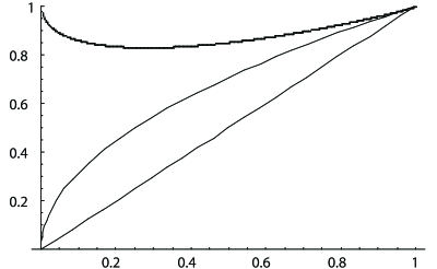
Figure 2: The graphs of $1-c(p)>\sqrt{p}>p$ for $0<p<1$

Appendix A Appendix: Estimation of the binomial coefficient

Lemma A.1.

Let $N$ be a positive integer and $\alpha,\beta,\gamma$ be real numbers with $\alpha,\beta\in(0,1)$ and $\gamma\in[0,1]$. Then,

$$\binom{(\alpha+\beta+\gamma)N}{\alpha N}\leq E(\alpha,\beta,\gamma,N)\left(\frac{(\alpha+\beta)^{\alpha+\beta}}{\alpha^{\alpha}\beta^{\beta}}\right)^{N},$$

where

$$E(\alpha,\beta,\gamma,N)=\sqrt{\frac{\alpha+\beta}{2\pi\alpha\beta N}}\exp\left\{\frac{1}{12(\alpha+\beta)N}+\gamma\left(1+\frac{\alpha}{\beta}\right)N\right\}.$$

Proof.

We use Stirling’s formula as given in [6, page 216]:

$$\sqrt{2\pi n}\left(\frac{n}{e}\right)^{n}\leq n!\leq e^{1/(12n)}\sqrt{2\pi n}\left(\frac{n}{e}\right)^{n}.$$

From this formula,

$$\binom{(\alpha+\beta+\gamma)N}{\alpha N}$$

$$\leq e^{1/(12(\alpha+\beta+\gamma)N)}\frac{\sqrt{2\pi(\alpha+\beta+\gamma)N}}{\sqrt{2\pi\alpha N}\sqrt{2\pi(\beta+\gamma)N}}\left(\frac{(\alpha+\beta+\gamma)N}{e}\right)^{(\alpha+\beta+\gamma)N}\left(\frac{e}{\alpha N}\right)^{\alpha N}\left(\frac{e}{(\beta+\gamma)N}\right)^{(\beta+\gamma)N}$$

$$\leq e^{1/(12(\alpha+\beta)N)}\sqrt{\frac{\alpha+\beta+\gamma}{2\pi\alpha(\beta+\gamma)N}}\frac{\left(\alpha+\beta+\gamma\right)^{(\alpha+\beta+\gamma)N}}{\alpha^{\alpha N}\left(\beta+\gamma\right)^{(\beta+\gamma)N}}$$

Since $\frac{\alpha+\beta+\gamma}{\alpha(\beta+\gamma)}\leq\frac{\alpha+\beta}{\alpha\beta}$,

$$\binom{(\alpha+\beta+\gamma)N}{\alpha N}$$

$$\leq e^{1/(12(\alpha+\beta)N)}\sqrt{\frac{\alpha+\beta}{2\pi\alpha\beta N}}\left(\frac{\left(\alpha+\beta+\gamma\right)^{(\alpha+\beta+\gamma)}}{\alpha^{\alpha}\left(\beta+\gamma\right)^{(\beta+\gamma)}}\right)^{N}$$

$$\leq e^{1/(12(\alpha+\beta)N)}\sqrt{\frac{\alpha+\beta}{2\pi\alpha\beta N}}\left(\frac{\left(\alpha+\beta\right)^{\alpha+\beta}}{\alpha^{\alpha}\beta^{\beta}}\right)^{N}\left(\left(\frac{\alpha+\beta+\gamma}{\alpha+\beta}\right)^{\alpha+\beta}\left(\frac{\beta}{\beta+\gamma}\right)^{\beta}\left(\frac{\alpha+\beta+\gamma}{\beta+\gamma}\right)^{\gamma}\right)^{N}$$

$$\leq \left(\frac{\left(\alpha+\beta\right)^{\alpha+\beta}}{\alpha^{\alpha}\beta^{\beta}}\right)^{N}\sqrt{\frac{\alpha+\beta}{2\pi\alpha\beta N}}e^{1/(12(\alpha+\beta)N)}\left(\left(1+\frac{\gamma}{\alpha+\beta}\right)^{\alpha+\beta}\left(1+\frac{\alpha}{\beta}\right)^{\gamma}\right)^{N}$$

Because $1+x\leq e^{x}$,

$$\binom{(\alpha+\beta+\gamma)N}{\alpha N}\leq\left(\frac{\left(\alpha+\beta\right)^{\alpha+\beta}}{\alpha^{\alpha}\beta^{\beta}}\right)^{N}\sqrt{\frac{\alpha+\beta}{2\pi\alpha\beta N}}e^{1/(12(\alpha+\beta)N)}\exp\left\{\gamma N+\gamma\frac{\alpha}{\beta}N\right\}\qed$$

Corollary A.2.

Let $p,c$ be fixed and let $r=cv$, with $v\to\infty$.

$$\binom{rv+2p\binom{v}{2}+2v\sqrt{2\ln v}}{rv}\leq\left((1+o(1))\left(\frac{(c+p)^{c+p}}{c^{c}p^{p}}\right)\right)^{v^{2}}.$$

Proof.

$$\binom{rv+2p\binom{v}{2}+2v\sqrt{2\ln v}}{rv}=\binom{cv^{2}+pv^{2}-pv+2v\sqrt{2\ln v}}{cv^{2}}.$$

Let $N=v^{2}$, $\alpha=c$, $\beta=p$, and $\gamma=\frac{1}{v^{2}}(-pv+2v\sqrt{2\ln v})$. With $p$ and $c$ fixed, by Lemma A.1 we see that

$$\binom{rv+2p\binom{v}{2}+2v\sqrt{2\ln v}}{rv}\leq\left((1+o(1))\left(\frac{(c+p)^{c+p}}{c^{c}p^{p}}\right)\right)^{v^{2}}.\qed$$

Appendix B Appendix: Connectivity is minimum degree

Bollobás and Thomason [8] proved that for $G\sim G(v,p)$, regardless of $p$, then $\Pr[\kappa(G)<\delta(G)]\rightarrow 0$ as $v\rightarrow\infty$. Bollobás [5] proved the result for $p$ in a restricted interval, but the statement of his theorem is much more general. For our result, we need to bound the probability that $\kappa(G)=\delta(G)$ where $G\sim G(v,p)$, but need the result only for a fixed $p$.

Lemma B.1.

Let $p\in(0,1)$ be fixed and $G$ be distributed according to $G(v,p)$. If $v$ is sufficiently large, then

$$\Pr[\kappa(G)<\delta(G)]\leq 3v^{-2}.$$

Proof.

Let $\delta=\delta(G)$. By Theorem 3.2 we see that, with probability at least $1-v^{-2}$,

$$\delta\leq\frac{2e(G)}{v}\leq\frac{2\left(p\binom{v}{2}+v\sqrt{2\ln v}\right)}{v}=p(v-1)+2\sqrt{2\ln v}\leq pv+2\sqrt{2\ln v}.$$ (9)

For the remainder of the proof we assume $\delta\leq pv+2\sqrt{2\ln v}.$

If $\kappa(G)<\delta$, then there exists a partition $V(G)=V_{1}\cup S\cup V_{2}$ such that $|S|<\delta$, $2\leq|V_{1}|\leq|V_{2}|$ and there is no edge between $V_{1}$ and $V_{2}$. Let the closed neighborhood of vertex $x$ be denoted $N[x]$ and be equal to $\{x\}\cup N(x)$.

We will show first that there is an integer $t$ such that the probability that $2\leq|V_{1}|\leq t$ is at most $v^{-2}$ (we will determine the value of $t$ later). By a different calculation, we will then show that the probability that $t<|V_{1}|\leq(v+\delta)/2$ is also at most $v^{-2}$. Note that we don’t attempt to optimize the probability or to give a range of $p$ over which these conditions hold. A total probability of $2v^{-2}$ is sufficient for our purposes and results in an easier proof.

The event $\{2\leq|V_{1}|\leq t\}$ can occur only if there are two distinct vertices, $x_{1}$ and $x_{2}$, such that the cardinality of the union of their closed neighborhoods is less than $t+\delta$. For vertices $y_{i}\in V(G)\backslash\{x_{1},x_{2}\}$, let $Y_{i}$ be independent indicator variables for $y_{i}\in N[x_{1}]\cup N[x_{2}]$. Since the probability $y_{i}\notin N[x_{1}]\cup N[x_{2}]$ is $(1-p)^{2}$,

$${\bf E}[|N[x_{1}]\cup N[x_{2}]|]={\bf E}[2+Y_{1}+\dots+Y_{v-2}]]=2+(v-2)(2p-p^{2}).$$

Hence, assuming $(t+\delta)-\left(2+(2p-p^{2})(v-2)\right)<0$, by the negative version of Theorem 3.1,

$$\Pr\left[2\leq|V_{1}|\leq t\right] \leq \binom{v}{2}\hbox to0.0pt{$\displaystyle\Pr\left[\left|N[x_{1}]\cup N[x_{2}]\right|<t+\delta\right]$\hss}$$

$$= \binom{v}{2}\Pr\left[\left|N[x_{1}]\cup N[x_{2}]\right|-\left(2+(2p-p^{2})(v-2)\right)<(t+\delta)-\left(2+(2p-p^{2})(v-2)\right)\right]$$

$$\leq \exp\left\{2\ln v-\frac{1}{2(v-2)}\left((t+\delta)-2-(2p-p^{2})(v-2)\right)^{2}\right\}.$$

Thus if $t+\delta\leq(2p-p^{2})(v-2)+2-3\sqrt{v\ln v}$, then $\Pr\left[2\leq|V_{1}|\leq t\right]<v^{-2}$.

Since $v\geq 2$ and we have assumed $\delta\leq pv+2\sqrt{2\ln v}$, we may set

$$t=(2p-p^{2})v-3\sqrt{v\ln v}-\delta\geq(2p-p^{2})v-3\sqrt{v\ln v}-pv-2\sqrt{2\ln v}\geq p(1-p)v-5\sqrt{v\ln v}.$$

We will use the bound $\binom{v}{i}\leq\left(\frac{ev}{i}\right)^{i}$ which is true for all $1\leq i\leq v$ [6, page 216], and the trivial bound $\binom{v-i}{\delta}\leq v^{\delta}$, which is true for all $v-i,\delta\geq 0$. The event $\{t<|V_{1}|\leq(v+\delta)/2\}$ has a probability which is bounded as follows:

$$\Pr\left[t<|V_{1}|\leq(v+\delta)/2\right] \leq \sum_{i=\lfloor t+1\rfloor}^{\lfloor(v+\delta)/2\rfloor}\binom{v}{i}\binom{v-i}{\delta}(1-p)^{i(v-i-\delta)}$$

$$\leq \sum_{i=\lfloor t+1\rfloor}^{\lfloor(v+\delta)/2\rfloor}\left(\frac{ev}{i}\right)^{i}v^{\delta}(1-p)^{i(v-\delta)/2}$$

$$\leq v^{\delta}\sum_{i=\lfloor t+1\rfloor}^{\lfloor(v+\delta)/2\rfloor}\left[ev(1-p)^{(v-\delta)/2}\right]^{i}$$

If $v$ is large enough, then $ev(1-p)^{(v-\delta)/2}<ev(1-p)^{(v-pv-2\sqrt{2\ln v})/2}<1$. Using this in our calculation, along with the bound $1-p\leq e^{-p}$,

$$\Pr\left[t<|V_{1}|\leq(v+\delta)/2\right] \leq v^{\delta}\sum_{i=\lfloor t+1\rfloor}^{\lfloor(v+\delta)/2\rfloor}\left[ev(1-p)^{(v-\delta)/2}\right]^{i}$$ (10)

$$\leq v^{\delta+1}\left[ev(1-p)^{(v-pv-2\sqrt{2\ln v})/2}\right]^{t}$$

$$\leq v^{\delta+1+t}e^{t}\exp\left\{-\frac{pvt}{2}+\frac{p^{2}vt}{2}+pt\sqrt{2\ln v}\right\}$$

$$\leq v^{v}e^{v}\exp\left\{-\frac{p(1-p)vt}{2}+pv\sqrt{2\ln v}\right\}$$

$$= \exp\left\{v\ln v+v+pv\sqrt{2\ln v}-\frac{p(1-p)}{2}vt\right\}$$

Since $t\geq p(1-p)v-5\sqrt{v\ln v}$, the expression in (10) is easily bounded above by $\exp\{-2\ln v\}$ for $v$ large enough.

Summarizing, if $v$ is large enough, then with probability at least $1-3v^{-2}$, there is no set $S$ of size less than $\delta$ such that $V(G)-S$ is disconnected. ∎

References

- [1] N. Alon and J.H. Spencer, The Probabilistic Method, second ed., John Wiley & Sons, New York, 2000.
- [2] American Institute of Mathematics workshop “Spectra of Families of Matrices described by Graphs, Digraphs, and Sign Patterns,” held October 23-27, 2006 in Palo Alto, CA. Workshop webpage: http://aimath.org/pastworkshops/matrixspectrum.html.
- [3] F. Barioli, S.M. Fallat, and L. Hogben, A variant on the graph parameters of Colin de Verdière: Implications to the minimum rank of graphs. Electron. J. Linear Algebra, 13 (2005), 387–404.
- [4] A. Berman, S. Friedland, L. Hogben, U.G. Rothblum and B. Shader, An upper bound for minimum rank of a graph, Linear Algebra Appl. 429 (2008), no. 7, 1629-1638.
- [5] B. Bollobás, Degree sequences of random graphs, Discrete Math. 33 (1981), no. 1, 1–19.
- [6] B. Bollobás, Modern Graph Theory. Graduate Texts in Mathematics, 184. Springer-Verlag, New York, 1998.
- [7] B. Bollobás, Random Graphs, second ed., Cambridge Studies in Advanced Mathematics, 73, Cambridge University Press, Cambridge, 2001.
- [8] B. Bollobás and A. Thomason, Random graphs of small order, in: Random Graphs ’83 (Poznań, 1983), North-Holland Math. Stud., 118, North-Holland, Amsterdam, 1985, pp. 47–97.
- [9] R. Brualdi, L. Hogben and B. Shader, AIM Workshop Spectra of Families of Matrices described by Graphs, Digraphs, and Sign Patterns, Final Report: Mathematical Results (revised, March 30, 2007). http://aimath.org/pastworkshops/matrixspectrumrep.pdf.
- [10] Y. Colin de Verdière, On a new graph invariant and a criterion for planarity, in: Graph Structure Theory, Contemporary Mathematics, vol. 147, American Mathematical Society, Providence, 1993, pp. 137–147.
- [11] Y. Colin de Verdière, Multplicities of eigenvalues and tree-width graphs, J. Combin. Theory Ser. B 74 (1998), no. 2, 121–146.
- [12] S. Fallat and L. Hogben, The minimum rank of symmetric matrices described by a graph: A survey, Linear Algebra Appl. 426 (2007) 558–582.
- [13] Hein van der Holst. Three-connected graphs whose maximum nullity is at most three. Linear Algebra and Its Applications 429 (2007), 625–632.
- [14] H. van der Holst, L. Lovász, and A. Schrijver, The Colin de Verdière graph parameter, in: Graph Theory and Computational Biology (Balatonlelle, 1996), Bolyai Soc. Math. Stud., 7, János Bolyai Math. Soc., Budapest, 1999, pp. 29–85.
- [15] L. Lovász, M. Saks and A. Schrijver, Orthogonal representations and connectivity of graphs, Linear Algebra Appl. 114/115 (1989), 439–454.
- [16] L. Lovász, M. Saks and A. Schrijver, A correction: “Orthogonal representations and connectivity of graphs,” Linear Algebra Appl. 313 (2000), no. 1-3, 101–105.
- [17] R. Pendavingh, On the relation between two minor-monotone graph parameters, Combinatorica, 18 (1998), no. 2, 281-292.
- [18] L. Rónyai, L. Babai and M.K. Ganapathy, On the number of zero-patterns of a sequence of polynomials, J. Amer. Math. Soc. 14 (2001), no. 3, 717–735 (electronic).
- [19] E. Shamir and J.H. Spencer, Sharp concentration of the chromatic number in random graphs , Combinatorica 7 (1987), no. 1, 121–129.