${\rm{Marcin\;Daszkiewicz}}$

Abstract

In this article, we investigate the impact of twisted space-time on the photoelectric effect, i.e., we derive the $\theta$-deformed threshold frequency. In such a way we indicate that the space-time noncommutativity strongly enhances the photoelectric process.

The suggestion to use noncommutative coordinates goes back to Heisenberg and was firstly formalized by Snyder in [1]. Recently, there were also found formal arguments based mainly on Quantum Gravity [2], [3] and String Theory models [4], [5], indicating that space-time at the Planck scale should be noncommutative, i.e., it should have a quantum nature. Consequently, there appeared a lot of papers dealing with noncommutative classical and quantum mechanics (see e.g. [6], [7]) as well as with field theoretical models (see e.g. [8], [9]), in which the quantum space-time is employed.

In accordance with the Hopf-algebraic classification of all deformations of relativistic [10] and nonrelativistic [11] symmetries, one can distinguish three basic types of space-time noncommutativity (see also [12] for details):

1) Canonical ($\theta^{\mu\nu}$-deformed) type of quantum space [13]-[15]

$$[\;{x}_{\mu},{x}_{\nu}\;]=i\theta_{\mu\nu}\;,$$ (1)

2) Lie-algebraic modification of classical space-time [15]-[18]

$$[\;{x}_{\mu},{x}_{\nu}\;]=i\theta_{\mu\nu}^{\rho}{x}_{\rho}\;,$$ (2)

and

3) Quadratic deformation of Minkowski and Galilei spaces [15], [18]-[20]

$$[\;{x}_{\mu},{x}_{\nu}\;]=i\theta_{\mu\nu}^{\rho\tau}{x}_{\rho}{x}_{\tau}\;,$$ (3)

with coefficients $\theta_{\mu\nu}$, $\theta_{\mu\nu}^{\rho}$ and $\theta_{\mu\nu}^{\rho\tau}$ being constants.

Moreover, it has been demonstrated in [12], that in the case of the so-called N-enlarged Newton-Hooke Hopf algebras $\,{\mathcal{U}}^{(N)}_{0}({NH}_{\pm})$ the twist deformation provides the new space-time noncommutativity of the form,

$${\bf 4)}\;\;\;\;\;\;\;\;\;[\;t,{x}_{i}\;]=0\;\;\;,\;\;\;[\;{x}_{i},{x}_{j}\;]=if_{\pm}\left(\frac{t}{\tau}\right)\theta_{ij}(x)\;,$$ (4)

with time-dependent functions

$$f_{+}\left(\frac{t}{\tau}\right)=f\left(\sinh\left(\frac{t}{\tau}\right),\cosh\left(\frac{t}{\tau}\right)\right)\;\;\;,\;\;\;f_{-}\left(\frac{t}{\tau}\right)=f\left(\sin\left(\frac{t}{\tau}\right),\cos\left(\frac{t}{\tau}\right)\right)\;,$$

$\theta_{ij}(x)\sim\theta_{ij}={\rm const}$ or $\theta_{ij}(x)\sim\theta_{ij}^{k}x_{k}$ and $\tau$ denoting the time scale parameter - the cosmological constant. Besides, it should be noted, that the above mentioned quantum spaces 1), 2) and 3) can be obtained by the proper contraction limit of the commutation relations 4).

In this article we investigate the impact of quantum space-times (4) on the photoelectric process described by the following equation [21]

$$K=\hbar\omega-W\;,$$ (5)

where $K$, $\hbar\omega$ and $W$ denote the kinematic energy of electron, energy quanta of light and work function, respectively. To this end, we assume that photons emitted by transplanckian (noncommutative) source are described by the nonrelativistic oscillator model [22] defined on the following twist-deformed N-enlarged Newton-Hooke phase space

$$[\;\hat{x}_{1},\hat{x}_{2}\;]=2if_{\kappa}({t})\;\;\;,\;\;\;[\;\hat{p}_{1},\hat{p}_{2}\;]=2ig_{\kappa}({t})\;,$$ (6)

$$[\;\hat{x}_{i},\hat{p}_{j}\;]=i\hbar\delta_{ij}\left[1+f_{\kappa}({t})g_{\kappa}({t})/\hbar^{2}\right]\;,$$ (7)

with an arbitrary function $g_{\kappa}({t})$. Then the corresponding Hamiltonian operator is given by

$$\hat{H}=\frac{1}{2m}\left({\hat{{p}}_{1}^{2}}+{\hat{{p}}_{2}^{2}}\right)+\frac{1}{2}m\omega^{2}\left({\hat{{x}}_{1}^{2}}+{\hat{{x}}_{2}^{2}}\right)\;.$$ (8)

with $m$ and $\omega$ denoting the mass and frequency of a particle, respectively. In terms of commutative variables $({x}_{i},{p}_{i})$, which correspond to the low-energy observer, it takes the form

$$\hat{H}=\hat{H}(t)=\frac{1}{2M(t)}\left({{{p}}_{1}^{2}}+{{{p}}_{2}^{2}}\right)+\frac{1}{2}M(t)\Omega^{2}(t)\left({{{x}}_{1}^{2}}+{{{x}}_{2}^{2}}\right)-S(t)L\;,$$ (9)

where

$$L=x_{1}p_{2}-x_{2}p_{1}\;,$$ (10)

$$1/M(t)=1/m+m\omega^{2}f_{\kappa}^{2}(t)/\hbar^{2}\;,$$ (11)

$$\Omega(t)=\Omega_{f}(\omega)=\sqrt{\left(1/m+m\omega^{2}f_{\kappa}^{2}(t)/\hbar^{2}\right)\left(m\omega^{2}+g_{\kappa}^{2}(t)/(\hbar^{2}m)\right)}\;,$$ (12)

and

$$S(t)=m\omega^{2}f_{\kappa}(t)/\hbar+g_{\kappa}(t)/(\hbar m)\;.$$ (13)

The corresponding energy spectrum can be find with the use of time-dependent creation/anni-hilation operator procedure and it looks as follows

$$E_{n_{+},n_{-}}(t)=\hbar\Omega_{+}(t)\left[n_{+}+\frac{1}{2}\right]+\hbar\Omega_{-}(t)\left[n_{-}+\frac{1}{2}\right]\;\;;\;\;n_{\pm}=0,1,2,\ldots\;,$$ (14)

with frequencies

$$\Omega_{\pm}(t) = \Omega(t)\mp S(t)\;.$$ (15)

Besides, one can observe that for functions $f_{\kappa}({t})$ and $g_{\kappa}({t})$ such that

$$f_{\kappa}(t)=-{g_{\kappa}(t)}/({\omega^{2}m^{2}})\;,$$ (16)

we have

$$E_{n_{+},n_{-}}(t)=\hbar\Omega(t)\left[n_{+}+\frac{1}{2}\right]+\hbar\Omega(t)\left[n_{-}+\frac{1}{2}\right]\;.$$ (17)

It means that the spectrum (14) becomes isotropic and the corresponding energy quanta takes the form

$$E_{quanta}=E_{n+1}-E_{n}=\hbar\Omega_{f}(\omega)\;.$$ (18)

Particularly, for the canonical deformation $f_{\kappa}(t)=\kappa=\theta={\rm const}$ we get

$$E_{n_{+},n_{-},\theta}=\hbar\Omega_{\theta}\left[n_{+}+\frac{1}{2}\right]+\hbar\Omega_{\theta}\left[n_{-}+\frac{1}{2}\right]\;,$$ (19)

with a constant frequency

$$\Omega_{\theta}=\Omega_{\theta}(\omega)=m\omega\left({1}/{m}+{m\omega^{2}}\theta^{2}/{\hbar^{2}}\right)\;,$$ (20)

for which $\lim_{\theta\to 0}\Omega_{\theta}=\omega$.

As mentioned above, in the hamiltonian function (8), the frequency $\omega$ corresponds to the frequency of emitted light described in terms of noncommutative variables $(\hat{x}_{i},\hat{p}_{i})$ associated with the Planck scale. However, the formula (18) gives the corresponding energy quanta (obviously different than $\hbar\omega$) in terms of commutative variables $({x}_{i},{p}_{i})$, i.e., it describes the deformed energy of a single photon which is detected by low-energy observer. It is simply the energy quanta which should be detected on a surface of metal in a typical laboratory room. In other words the formula (18) gives the energy of photons emitted for example by transplanckian (noncommutative) astrophysical sources which arrive to (commutative) Earth.

Consequently, in our further analysis, we exchange in (5) the quanta $\hbar\omega$ by the deformed ones $\hbar\Omega_{f}(\omega)$ such that

$$K=\hbar\Omega_{f}(\omega)-W=\hbar m\omega\left({1}/{m}+{m\omega^{2}}f^{2}_{\kappa}(t)/{\hbar^{2}}\right)-W\;.$$ (21)

One can see that the main difference between (5) and (21) concerns the shape of the function $K(\omega)$. In the first (undeformed) case it remains linear in the frequency $\omega$ while for the second process it forms the third degree polynomial. Next one can ask for so-called threshold quanta, i.e., for such an energy portion for which the frequency $\omega_{tr}$ satisfies

$$\hbar\omega_{tr}-W=0\;,$$ (22)

and

$$\hbar\Omega_{f}(\omega_{tr})-W=0\;,$$ (23)

respectively. The solution of (22) with respect to the frequency $\omega_{tr}$ seems to be trivial

$$\omega_{tr}=\frac{W}{\hbar}\;.$$ (24)

In the case of equation (23) the situation is more complicated. However, one can find its three roots - two of them are complex while the third one remains real; it looks as follows

$$\omega_{tr}(f_{\kappa}(t)) = \frac{\left(\sqrt{3}\sqrt{4\hbar^{6}m^{6}f_{\kappa}^{6}(t)+27\hbar^{2}m^{8}f_{\kappa}^{8}(t)W^{2}}+9\hbar m^{4}f_{\kappa}^{4}(t)W\right)^{1/3}}{(2^{1/3}3^{2/3}m^{2}f_{\kappa}^{2}(t))}+$$ (25)

$$- \frac{\left(\left(\frac{2}{3}\right)^{1/3}\hbar^{2}\right)}{\left(\sqrt{3}\sqrt{4\hbar^{6}m^{6}f^{6}_{\kappa}(t)+27\hbar^{2}m^{8}f_{\kappa}^{8}(t)W^{2}}+9\hbar m^{4}f_{\kappa}^{4}(t)W\right)^{1/3}}\;.$$

The solutions (24) and (25) define the threshold frequencies for processes (5) and (21), respectively.

Let us now turn to the simplest (canonical) deformation of the phase space (6), (7) such (as already mentioned) that

$$f_{\kappa}(t)=\theta={\rm const}\;.$$ (26)

Then, in accordance with the relation (16) we have

$$g_{\kappa}(t)=-\theta\omega^{2}m^{2}\;.$$ (27)

Consequently, in such a case, due to the formula (20), equation (21) takes the form

$$K=\hbar\Omega_{\theta}(\omega)-W=\hbar m\omega\left({1}/{m}+{m\omega^{2}}\theta^{2}/{\hbar^{2}}\right)-W\;,$$ (28)

while the corresponding threshold frequency $\omega_{tr}$ is equal to

$$\omega_{tr}(\theta) = \frac{\left(\sqrt{3}\sqrt{4\hbar^{6}m^{6}\theta^{6}+27\hbar^{4}m^{8}\theta^{8}W^{2}}+9\hbar^{2}m^{4}\theta^{4}W\right)^{1/3}}{(2^{1/3}3^{2/3}m^{2}\theta^{2})}+$$ (29)

$$- \frac{\left(\left(\frac{2}{3}\right)^{1/3}\hbar^{2}\right)}{\left(\sqrt{3}\sqrt{4\hbar^{6}m^{6}\theta^{6}+27\hbar^{4}m^{8}\theta^{8}W^{2}}+9\hbar^{2}m^{4}\theta^{4}W\right)^{1/3}}\;.$$

Obviously, for the deformation parameter $\theta$ approaching zero we should reproduce from (29) the standard relation (24). Besides we have (see Figure 1 and 2)

$$\lim_{\theta\to\infty}\omega_{tr}(\theta)=0\;,$$ (30)

which means that in our treatment the canonical noncommutativity strongly enhances the photoelectric effect.

                  

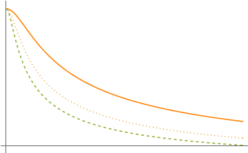
Figure 1: The shape of the threshold frequency $\omega_{tr}(\theta)$ for the three different values of the parameter $m$: $m=1$ (continuous line), $m=2$ (dotted line) and $m=3$ (dashed line). In all three cases we fix the work function $W=1$.

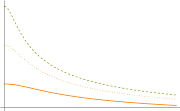
Figure 2: The shape of the threshold frequency $\omega_{tr}(\theta)$ for the three different values of the work function: $W=1$ (continuous line), $W=2$ (dotted line) and $W=3$ (dashed line). In all three cases we fix the parameter $m=1$.

References

• [1] H.S. Snyder, Phys. Rev. 72, 68 (1947)
• [2] S. Doplicher, K. Fredenhagen, J.E. Roberts, Phys. Lett. B 331, 39 (1994); Comm. Math. Phys. 172, 187 (1995); hep-th/0303037
• [3] A. Kempf and G. Mangano, Phys. Rev. D 55, 7909 (1997); hep-th/9612084
• [4] A. Connes, M.R. Douglas, A. Schwarz, JHEP 9802, 003 (1998); hep-th/9711162
• [5] N. Seiberg and E. Witten, JHEP 9909, 032 (1999); hep-th/9908142
• [6] A. Deriglazov, JHEP 0303, 021 (2003); hep-th/0211105
• [7] M. Chaichian, M.M. Sheikh-Jabbari, A. Tureanu, Phys. Rev. Lett. 86, 2716 (2001); hep-th/0010175
• [8] P. Kosinski, J. Lukierski, P. Maslanka, Phys. Rev. D 62, 025004 (2000); hep-th/9902037
• [9] M. Chaichian, P. Prešnajder and A. Tureanu, Phys. Rev. Lett. 94, 151602 (2005); hep-th/0409096
• [10] S. Zakrzewski, ”Poisson Structures on the Poincare group”; q-alg/9602001
• [11] Y. Brihaye, E. Kowalczyk, P. Maslanka, ”Poisson-Lie structure on Galilei group”; math/0006167
• [12] M. Daszkiewicz, Mod. Phys. Lett. A27 (2012) 1250083; arXiv: 1205.0319 [hep-th]
• [13] R. Oeckl, J. Math. Phys. 40, 3588 (1999)
• [14] M. Chaichian, P.P. Kulish, K. Nashijima, A. Tureanu, Phys. Lett. B 604, 98 (2004); hep-th/0408069
• [15] M. Daszkiewicz, Mod. Phys. Lett. A 23, 505 (2008); arXiv: 0801.1206 [hep-th]
• [16] J. Lukierski, A. Nowicki, H. Ruegg and V.N. Tolstoy, Phys. Lett. B 264, 331 (1991)
• [17] S. Giller, P. Kosinski, M. Majewski, P. Maslanka and J. Kunz, Phys. Lett. B 286, 57 (1992)
• [18] J. Lukierski and M. Woronowicz, Phys. Lett. B 633, 116 (2006); hep-th/0508083
• [19] O. Ogievetsky, W.B. Schmidke, J. Wess, B. Zumino, Comm. Math. Phys. 150, 495 (1992)
• [20] P. Aschieri, L. Castellani, A.M. Scarfone, Eur. Phys. J. C 7, 159 (1999); q-alg/9709032
• [21] A. Einstein, Annalen der Physik 17, 132 (1905)
• [22] M. Daszkiewicz, Chin. J. Phys. 53 (2015) 120002; arXiv: 1512.08859 [hep-th]
Refer to caption