Forecasts for the WFIRST High Latitude Survey using the BlueTides Simulation

Abstract

We use the BlueTides simulation to predict the properties of the high-$z$ galaxy and active galactic nuclei (AGN) populations for the planned 2200deg² Wide-Field Infrared Survey Telescope’s (WFIRST)-AFTA High Latitude Survey (HLS). BlueTides is a cosmological hydrodynamic simulation, which incorporates a variety of baryon physics in a $(400h^{-1}\mathrm{Mpc})^{3}$ volume evolved to $z=8$ with 0.7 trillion particles. The galaxy luminosity functions in the simulation show good agreement with all the current observational constraints (up to $z=11$) and predicts an enhanced number of UV bright galaxies. At the proposed depth of the HLS ($m<26.75$), BlueTides predicts $10^{6}$ galaxies at $z=8$ with a few up to $z\sim 15$ due to the enhanced bright end of the galaxy luminosity function. At $z=8$, galaxies in the mock HLS have specific star formation rates of $\sim 10{\rm Gyr}^{-1}$ and ages of $\sim 80{\rm Myr}$ (both evolving linearly with redshift) and a non-evolving mass-metallicity relation. BlueTides also predicts $\sim 10^{4}$ AGN in WFIRST HLS from $z=8$ out to $z\sim 14$. These AGN host black holes of $M\sim 10^{6}-10^{8}M_{\odot}$ accreting close to their Eddington luminosity. Galaxies and AGN have host halo masses of $M_{halo}\sim 10^{11-12}M_{\odot}$ and a linear bias $b\approx 13-20$. Given the expected galaxy space densities, their high bias and large volume probed we speculate that it may be feasible for WFIRST HLS detect the Baryon Acoustic Oscillation peak in the galaxy power spectrum out to $z=8-9$.

Parameter	Value	Description
$\Omega_{\Lambda}$	0.7186	Vacuum energy density
$\Omega_{m}$	0.2814	Matter density
$\Omega_{b}$	0.0464	Baryon density
$h$	0.697	Dimensionless Hubble parameter
$n_{s}$	0.971	Spectral index
$\sigma_{8}$	0.82	Linear mass dispersion at $8h^{-1}$ Mpc
L	$400h^{-1}$ Mpc	Length of one edge of the simulation box
N	$2\times 7040^{3}$	Initial number of gas and dark matter particles
$M_{DM}$	$1.2\times 10^{7}h^{-1}$ Mpc	Mass of one dark matter particle
$M_{Gas}$	$2.36\times 10^{6}h^{-1}$ Mpc	Mass of one gas particle
$M_{BH}$	$5\times 10^{5}h^{-1}$ Mpc	Seed mass of black hole particles

Table 1: Important parameters for the BlueTides simulation. BlueTides uses the cosmology from the Wilkinson Microwave Anisotropy Probe nine-year data release (Hinshaw et al., 2013).

1 Introduction

At the current high redshift observational frontier ($z\sim 6-10$) there is, excitingly, evidence for a substantial population of galaxies (see the compilation by Bouwens et al. (2015) (hereafter B15) and references therein), with glimpses of intriguing properties seen (Oesch et al., 2014a; Holwerda et al., 2013). These observations provide initial measurements of the galaxy luminosity function (LF) (B15; Oesch et al., 2014a; McLeod et al., 2015) relying on around $\sim 100$ galaxies at redshift $z=8$ but fewer beyond redshift $z=9$. However, the 2 arcmin wide IR field of view of HST WFC3 has meant that cosmic variance is a dominant component of many observational studies, making clustering measures and searches for rare objects extremely difficult. The James Webb Space Telescope (JWST) will increase the depth to which we observe in deep fields of view, but cosmic variance will likely still persist. However, the Wide-Field Infrared Survey Telescope (WFIRST-AFTA) will transform the field, resolving these issues by providing depth comparable to that of HST Ultra Deep Fields with a field of view comparable to that of a ground based survey.

Spergel et al. (2013) (hereafter S13) reports an expected $10\sigma$ and $5\sigma$ limiting magnitude of $26$ and $26.75$ respectively, which is comparable to that of the HST. The WFIRST High Latitude Survey (HLS) is planned to have a 2200 deg² field of view, which will dramatically increase the number of galaxies available at redshifts $z=8$ and above. The WFIRST HLS will map this large portion of the sky in four NIR passbands (Y, J, H, and F184) and will include a slitless spectroscopic survey component that will obtain $R=\lambda/\Delta\lambda=600$ spectra allowing redshift measurements for these deep field objects. The observation of these high redshift galaxies are critical for our understanding of the first galaxies as well as their role in the epoch of reionization.

Numerical simulations, required to make theoretical predictions for these early times, are lacking however, particularly those with the dynamic range to cover both the formation of individual objects and make large scale statistical studies of them. Over the last few years, several large volume cosmological simulations of galaxy formation have been performed to study structure growth in the universe, galaxy formation, and reionization. MassiveBlack I ran a $533h^{-1}\rm Mpc$ side-length box to a redshift $z=4.75$ (Di Matteo et al., 2012). MassiveBlack II reduced the boxsize to $100h^{-1}\rm Mpc$ but had an improved resolution and ran all the way to redshift $z=0$ (Khandai et al., 2015). Illustris (Nelson et al., 2015) and the EAGLE simulation (Schaye et al., 2015) are both similar in size to Massive Black II but with different subgrid physics processes and feedback mechanisms.

With our newest simulation, BlueTides (Feng et al. 2016, hereafter F16, and Feng et al. 2015) (and the recent radical updates to the code efficiency, smoothed particle hydrodynamics formulation and star formation modeling) we have reached an unprecedented combination of volume and resolution. This enables us to cover the evolution of most of the galaxy mass function for the first billion years of cosmic history. We now are able to meet the challenge of simulating the next generation space telescope fields.

Cosmological simulations such as BlueTides are especially relevant to the high redshift observational frontier. This can be seen if we consider the recent discovery of the highest redshift galaxy to date. Oesch et al. (2016) observed a remarkably bright ($M_{\rm UV}=-22.1$) $z=11$ galaxy, GN- $z11$, in the CANDLES/GOODS-N imaging data. Extrapolations from lower redshift observations suggest that these UV bright galaxies should be exceedingly rare (0.06 per HST field of view in the best case) by $z=11$. BlueTides, however, predicts a significant probability of observing a galaxy like GN-$z11$ in the HST field of view ($\sim 13$ per cent). The BlueTides galaxies with $M_{\rm UV}\approx-22$ also match the inferred properties of GN-$z11$ such as the age, mass, and star formation rate (Waters et al., 2016).

In this work, we use BlueTides to predict the properties of the galaxy and active galactic nuclei (AGN) populations that will be discovered by the WFIRST HLS and their clustering at $8<z<15$. In Section 2 we discuss the spectral synthesis models we use to process the star formation, metallicity and stellar ages from from BlueTides to determine galaxy luminosities. We present a simple, self-consistent model for dust extinction, and also find AGN luminosities. We present the BlueTides forecasts of the photometric properties of galaxies detectable by the WFIRST HLS at $z>8$ in Section 3. In Section 4 we present the BlueTides predictions for the galaxy and AGN properties in the WFIRST HLS. We discuss the clustering properties and bias of these galaxies in Section 5 and conclude in Section 6.

2 The BlueTides Simulation

With BlueTides (and the BlueWaters supercomputer at the National Center for Supercomputing Applications) a qualitative advance has been possible: we have been able to run the first complete simulation (at least in terms of the hydrodynamics and gravitational physics) of the creation of the first galaxies and large-scale structures in the universe. The application required essentially the full BlueWaters system: we used 20,250 nodes (648,000 core equivalents). In order to effectively use the resources, a number of improvements had to be applied to the cosmological code P-Gadget3 (Springel, 2005) to make P(eta)-Gadget, now MP-Gadget, which is now fully instrumented to run on Peta-scale resources (F16). The major updates to the parallel infrastructure allowed operation at BlueWaters scale. The simulation code uses the pressure-entropy formulation of smoothed particle hydrodynamics (Hopkins, 2013) to solve the Euler equations. The $(400h^{-1}\text{Mpc})^{3}$ cubic simulation volume resulted in more than 200,000 star forming galaxies at redshift $z=8$. Halos were identified using a Friends-of-Friends algorithm with a linking length of 0.2 times the mean particle separation (Davis et al., 1985). Table 1 shows some of the basic cosmological and computational values for BlueTides.

A variety of sub-grid physical processes were implemented to study their effects on galaxy formation:

• star formation based on a multi-phase star formation model (Springel & Hernquist, 2003) with several effects following Vogelsberger et al. (2013)

• gas cooling through radiative transfer (Katz et al., 1996) and metal cooling (Vogelsberger et al., 2014)

• formation of molecular hydrogen and its effects on star formation (Krumholz & Gnedin, 2011)

• type II supernovae wind feedback (same model used in Illustris (Nelson et al., 2015))

• AGN feedback using the same model used in MassiveBlack I and II (Di Matteo et al., 2005)

• a "patchy" model of reionization (Battaglia et al., 2013) with a fiducial model of mean reionization redshift $z\approx 10$ (Hinshaw et al., 2013) with a UV background estimated by Faucher-Giguère et al. (2009)

These sub-grid baryon-physics processes are important for determining the photometric properties of high redshift galaxies and were shown to produce results consistent with observations in F16. In this section, we present the methods used to perform the post-processing of BlueTides in order to forecast the photometric and clustering properties of the galaxies detectable by WFIRST.

2.1 Galaxy Luminosities and Dust Attenuation

Our methodology of producing synthetic galaxy photometry is detailed in Wilkins et al. (2016). In brief: galaxy spectral energy distributions (SEDs) are calculated first by assigning a pure-stellar SED to each star particle according to its age and metallicity. We make use of the PEGASE v2 (Fioc & Rocca-Volmerange, 1997) stellar population synthesis (SPS) model assuming a Chabrier (2003) initial mass function (IMF). We note however that the choice of SPS model can affect predicted UV luminosities by up to 0.1 dex (Wilkins et al., 2016). Assuming a Salpeter IMF, instead of a Chabrier (2003) IMF, results in luminosities approximately 0.2 dex lower.

To model dust attenuation we utilize a scheme inspired by Jonsson (2006), where the metal density is integrated along parallel lines of sight. The dust attenuation is assumed to be proportional to the surface density of metal along the line of sight,

$$\tau_{V}(x,y,z)=\kappa\Sigma(x,y,z)=\int_{0}^{z}dz^{\prime}\kappa\rho_{\mathrm{metal}}(x,y,z^{\prime})$$ (1)

where $\tau_{V}(x,y,z)$ is the dust optical depth, $\rho_{\mathrm{metal}}(x,y,z^{\prime})$ is the metal density, $\kappa$ is a normalization factor, and we have chosen the $z$ direction as the the line of sight direction. The dust attenuation is then applied at subsequent redshifts (for more details see Wilkins et al. in-prep).

This simple model is calibrated so that we reproduce the bright end of the $z\sim 8$ UV LF from B15 (we naturally reproduce the faint end where we predict very little attenuation). It is however important to note that simply linking the metal density to the dust optical depth may not fully capture the redshift and luminosity/mass dependence of dust attenuation. This is because the production of dust is not expected to fully trace the production of metals (e.g. Mancini et al., 2015) with the expectation of lower dust-to-metal ratios at earlier times, and thus lower attenuation at high redshift. This is supported by the recent discovery of GN$-z11$ (Oesch et al., 2016; Waters et al., 2016). In the rest of this work, we present the predictions for both the dust corrected and intrinsic LF of galaxies in BlueTides for all redshifts.

2.2 Active Galactic Nuclei

Supermassive black holes were seeded in BlueTides with an initial mass of $5\times 10^{5}h^{-1}M_{\odot}$ once a halo reached a mass greater than $5\times 10^{10}h^{-1}M_{\odot}$. BlueTides tracks the rate at which mass is accreted from the halo onto the super-massive blackhole and from that a bolometric luminosity can be found. The blackhole bolometric luminosity is computed by assuming a mass-to-light conversion efficiency $\eta=0.1$:

$$L=\eta c^{2}\frac{dM_{\rm BH}}{dt}$$ (2)

where $L$ is the bolometric luminosity and $M_{\rm BH}$ is the mass of the black hole. Black holes in the BlueTides simulation were limited to having a mass accretion rate of three times that of their Eddington limit, given by $\dot{M}_{\mathrm{edd}}=4\pi GcM_{\rm BH}m_{p}/\sigma_{T}$ where $G$, $c$, $m_{p}$, and $\sigma_{T}$ are Newton’s constant, the speed of light, the mass of the proton, and the Thomson scattering cross section, respectively. The UV magnitude of the AGN is determined by (Fontanot et al., 2012):

$$M_{\rm UV}=-2.5\log_{10}\frac{L}{f_{\rm bol}\nu_{\rm B}}+34.1+\Delta_{\rm B,UV}$$ (3)

where $f_{\rm bol}=10.2$ is the bolometric correction (Elvis et al., 1994), $\nu_{\rm B}=6.74\times 10^{14}{\rm Hz}$, and $\Delta_{\rm B,UV}=-0.48$.

2.3 Clustering

Utilizing the spatial positions of galaxies in the BlueTides simulation, we compute the two-point spatial correlation function $\xi_{\mathrm{gg}}(r)$. For a particular redshift, we use all galaxies brighter than the WFIRST magnitude limit in the periodic volume of the box and use direct pair counts to measure $\xi_{\mathrm{gg}}(r)$. We also compute the dark matter correlation function, $\xi_{\mathrm{dm}}(r)$ using a Fast Fourier Transform based algorithm .

For each redshift we compute the linear bias defined by

$$b=\sqrt{\frac{\xi_{\mathrm{gg}}(r)}{\xi_{\mathrm{dm}}(r)}}$$ (4)

We compute $b$ by averaging equation 4 between the distances $r=10h^{-1}\mathrm{Mpc}$ and $r=75h^{-1}\mathrm{Mpc}$ to stay in the linear regime.

3 The WFIRST HLS Galaxy Population

3.1 Predicted Luminosity Functions

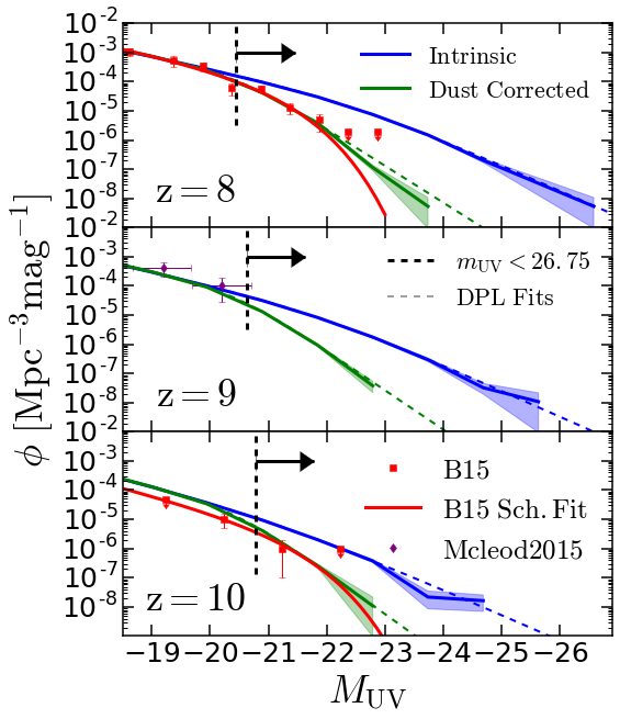
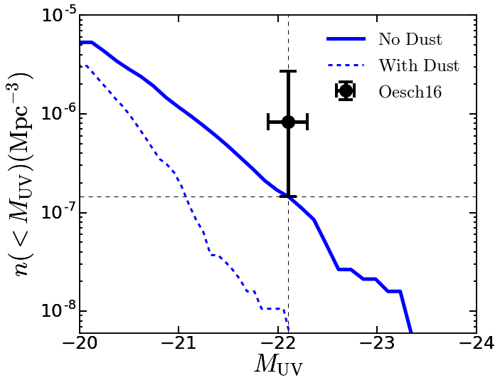
Figure 1: Top Panel: Comparison of the intrinsic (solid blue lines) and dust corrected (solid green lines) BlueTides LFs to available observational data from B15 (red data points) and McLeod et al. (2015) (purple data points). Shaded regions show the $1\sigma$ Poisson errors. Also shown are the best DPL fits (dashed blue and green lines) to the BlueTides LFs and the Schechter fits to observation data from B15 (red lines). The galaxies to the right of the dashed black lines are those that are UV bright enough to be detected by WFIRST. Bottom Panel: BlueTides prediction for the number density of objects like GN-$z11$. The error bar on the Oesch et al. (2016) point is a simple Poisson error.

The intrinsic and dust corrected LFs from the galaxies in BlueTides are shown in Figure 1 for $z=8$, 9 and 10, with Poisson errors given by the shaded regions. The dashed blue and green lines show a double power law (DPL) fit to the BlueTides intrinsic and dust corrected LFs, respectively. We note that a standard Schechter function does not represent a good description of the UV LF in BlueTides as it consistently under predicts the bright end (with and without accounting for dust). Here we use a DPL (B15; Bowler et al., 2014) defined by:

$$\phi(M)=\frac{\phi^{*}}{10^{0.4(\alpha+1)(M-M^{*})}+10^{0.4(\beta+1)(M-M^{*})}}$$ (5)

where $\phi^{*},M^{*},\alpha,{\rm and\ }\beta$ are the normalization, characteristic magnitude, faint end slope, and bright end slope, respectively. Results and the parameters of the DPL fits are presented in the Appendix.

The data points in Figure 1 show the observations compiled by B15 and McLeod et al. (2015). The red line is the best fit Schechter function as provided by B15. The arrows in the left-hand-side of the plot in Figure 1 indicate the planned $5\sigma$ detection limit of WFIRST HLS. We note that the current observational data shows no deviation from a Schechter-like LF at these high redshifts (see also discussion in B15). However, the bright end ($M_{\rm UV}<-21$) of the UV LF at $z>8$ is largely unconstrained observationally. BlueTides predicts a deviation from a Schechter LF in the WFIRST galaxy population. In particular, the number of objects predicted for the bright end of the LF is significantly enhanced compared to those expected from the extrapolation of the Schechter fit to current observational data.

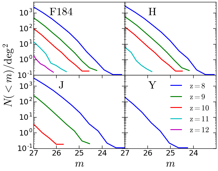
Figure 2: Surface density photometry for the WFIRST HLS band passes. Luminosities bey ond the Lyman break limit have been set to zero for the appropriate redshift in each band.

The BlueTides prediction of an enhanced number of bright sources is supported by the recent discovery by Oesch et al. (2016) of the $M_{\rm UV}=-22.1$ galaxy at $z=11$ (see Waters et al., 2016). In the bottom panel of Fig 1 we show the number density inferred by Oesch et al. (2016) at $z=11$ compared to the BlueTides prediction (with and without dust). The BlueTides predictions using the intrinsic LFs is consistent with the observation of this incredibly massive $z=11$ galaxy (Waters et al., 2016). Note also that our dust correction model reduces the number density of objects like GN-z11 by an order of magnitude, making it largely incompatible with the observation of Oesch et al. (2016) and likely implying an increasingly negligible amount of dust at these redshifts (see also Section 2.1).

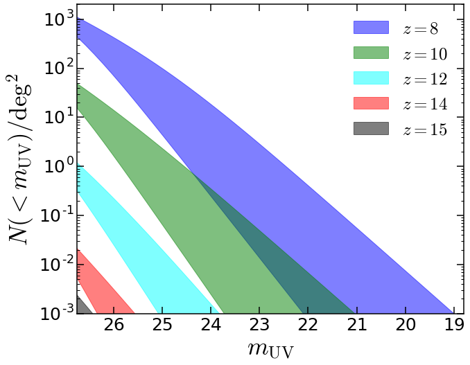
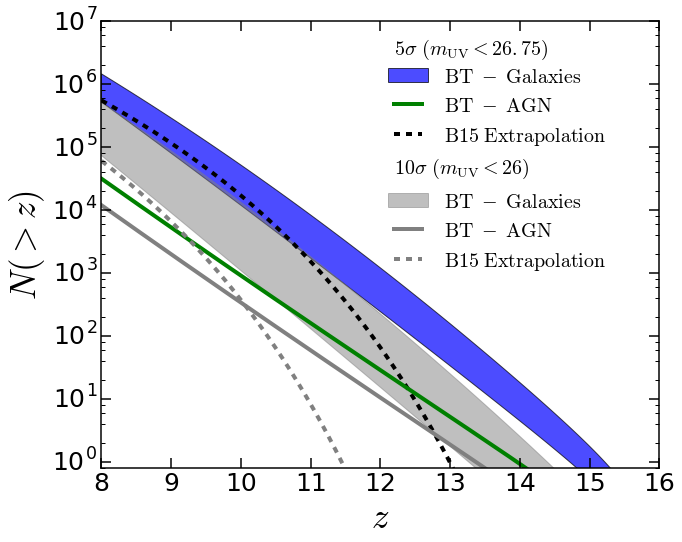
Figure 3: Top Panel: Surface density for $z=8$ and beyond. The results for $z=9,11,$ and $13$ are left out for clarity. The WFIRST field of view is $\sim 2200{\rm deg}^{2}$, so will be able to detect galaxies out to $z=15$ according to the BlueTides LF results. Our dust model is too extreme by $z=10$, so the lower limit at these redshifts are very conservative estimates. Bottom Panel: Predicted number of galaxies in the WFIRST HLS at or above a given redshift. The predictions shown are for the BlueTides galaxies (blue region) and AGN (green line) for the $5\sigma$ limit. Extrapolation of the B15 $z=8$ Schecther function is also shown (black dashed line). The grey lines show the same quantities but for the $10\sigma$ limit.

3.2 Expected Number of Galaxies in the HLS

Given the calculted SEDs for each galaxy in BlueTides  Figure 2 shows the predicted photometry (without dust corrections) for the F184(1.683-2.000 µm), H (1.380-1.774 µm), J (1.131-1.454 µm), and Y (0.927-1.192 µm) bands which are used in the WFIRST HLS for galaxy selection (S13) in the BlueTides volume. For redshifts $z=9-12$ we have set the luminosities at wavelengths beyond the Lyman break to zero to account for absorption by the intergalactic medium.

In order to make predictions for the total number of galaxies in the HLS we use the the DPL fits to the BlueTides LFs to extrapolate to the bright end. This is necessary as The WFIRST HLS has a much larger observational volume than the BlueTides simulation cube (approximately by a factor of 400). The number of galaxies per unit solid angle between $z_{1}$ and $z_{2}$ brighter than absolute magnitude $M$ is simply given by

$$N=\int_{z_{1}}^{z_{2}}dz\ r^{2}\frac{dr}{dz}\int_{-\infty}^{M}dM^{\prime}\phi(M^{\prime},z)\ sr^{-1}$$ (6)

where $r=r(z)$ is the comoving distance to redshift $z$. In the top panel of Figure 3 we show the expected surface densities in the WFIRST HLS as a function of the rest-frame UV luminosities (for all magnitudes less than the WFIRST $5\sigma$ limit). We calculate the surface density at each redshift $z$ with equation 6 between redshift $z-0.5$ and $z+0.5$ as a function of apparent magnitude. The upper (lower) limits at each redshift are from the LF without (with) dust correction. We give redshift evolution fits for the number densities in the Appendix.

The bottom panel of Figure 3 shows the total cumulative number of galaxies above a given redshift for the $5\sigma$ and $10\sigma$ WFIRST limits. We calculate the cumulative number for each redshift using equation 6 with a magnitude limit at each redshift that corresponds to the appropriate WFIRST limit. For comparison we also show the results for the cumulative number obtained using the B15 $z=8$ Schechter function best fit considering an optimistic evolution ($dM^{*}/dz=0.36$ as in S13) of the characteristic magnitude. The pessimistic evolution from S13 ($dM^{*}/dz=1.06$) significantly under fits the $z=10$ results from B15 and are therefore not considered. The BlueTides LFs predicts a comparable total number of galaxies as the B15 extrapolation but BlueTides predicts objects out to a significantly higher redshift. This is a result of the near identical normalizations of the BlueTides and B15 $z=8$ LFs, but an enhanced bright end in BlueTides compared to the extrapolation of observed constraints. BlueTides predicts a total of $10^{6}$ galaxies beyond $z=8$, and up to a few at $z=14-15$ at the planned depth and area of the WFIRST HLS. Without much dust, WFIRST will detect galaxies out to $z=15$ at the $5\sigma$ level.

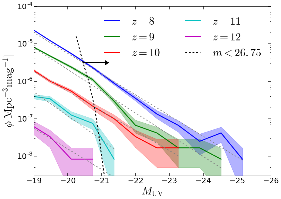
Figure 4: AGN LFs for BlueTides. Shaded regions show the $1\sigma$ Poisson errors. Grey dashed lines show a best fit to a power law LF. The black arrow and dashed line indicates the galaxies that are UV brighter than the WFIRST $5\sigma$ limit.

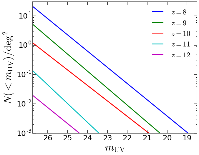
Figure 5: AGN surface densities according to BlueTides for AGN that have an intrinsic brightness above the WFIRST $5\sigma$ limit (no dust correction assumed).

3.3 Expected Number of AGN

The proposed survey area and depth of the WFIRST HLS will allow for the discovery of substantial populations of high-$z$ AGN. Currently the highest redshift known quasar is at $z=7.1$ (Mortlock et al., 2011) and only a handful of objects known at $z>6$ from SDSS (Fan et al., 2006). The limited knowledge of high-$z$ black holes will be revolutionized by WFIRST HLS. Using the black hole population simulated in BlueTides we examine the predictions for the LF and the expected number of AGN in the HLS at $z\geq 8$. Figure 4 shows the intrinsic UV LF for AGN in BlueTides with the dashed black line indicating the detection limit of WFIRST HLS. In order to predict the total number of AGN expected in the field of the HLS we fit the AGN LFs to a power law which we can then extrapolate to obtain the surface density of AGN above a given magnitude for those AGN beyond the $5\sigma$ cutoff for WFIRST (Figure 5). Figure 3 (green and grey lines) shows tens of thousand of AGN could be detectable at the $5\sigma$ level, with the brightest AGN out to $z=13-14$.

4 WFIRST Galaxy and AGN Properties

In this section, we examine a number of fundamental properties of the galaxy and AGN population predicted in the WFIRST HLS by BlueTides.

4.1 Galaxy Properties

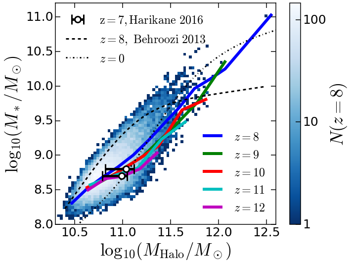
Figure 6: Stellar mass vs halo mass for the WFIRST galaxy population as predicted by BlueTides. Dashed lines show results from abundance matching by Behroozi et al. (2013). Data points show the $z=7$ results from Harikane et al. (2016). The 2D histogram shows the distribution of galaxies in the BlueTides volume at $z=8$. Solid lines show the mean in bins of $M_{\rm Halo}$ for the higher redshifts as indicated in the figure.

In Figure 6, we show the stellar - halo mass relation for the galaxies in BlueTides. Galaxies detected in our mock HLS have stellar masses between $10^{8}-10^{10}M_{\odot}$ that are hosted by dark matter halos with masses of $10^{10.5}-10^{12}M_{\odot}$ which are correlated with each other. The mean is well fit by a power law at each redshift, $M^{*}=(M_{h}/M_{0})^{\alpha}$ where the slope shows mild redshift evolution ($\alpha\approx-0.2(1+z)+2.8$). We compare the relation in BlueTides with the abundance matching results from Behroozi et al. (2013) at $z=0$ and extrapolated to $z=8$. The galaxy population in BlueTides appears somewhat closer to $z=0$ relation but perhaps showing less prominent signs of quenching at the high mass end. It is interesting to note that the predicted relation is in agreement with the halo occupation distribution modeling results (Harikane et al., 2016). The $z=7$ stellar - halo mass relation of Harikane et al. (2016) comes from the observations of around 300 Lymann break galaxies in the GOODS-N and GOODS-S fields. They split their $z=7$ sample into two subsamples ($m_{\rm UV}<28.2$ and $m_{\rm UV}<28.4$) each with around 100 galaxies and occupy halos with a model that assumes the number of galaxies in a given halo only depends on the halo mass.

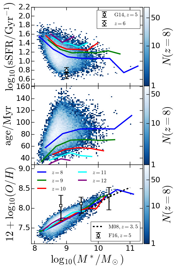
Figure 7: Galaxy properties for those bright enough to be detected by WFIRST. The 2D histogram shows the distribution of galaxies in the BlueTides volume at $z=8$. The solid lines show the mean values in bins of stellar mass. sSFR observations come from González et al. (2014). Best fit to metallicity measurements at $z=3.5$ come from Maiolino et al. (2008) and observations at $z=5$ come from Faisst et al. (2016).

In Figure 7 we show various galaxy properties from $z=8$ to $12$. The top panel shows the specific star formation rate (SFR$/M^{*}$) as a function of stellar mass. SFR$/M^{*}$ shows a strong evolution with redshift with a dependence ${\rm sSFR}\approx[4.1(1+z)-24.5]\ {\rm Gyr}^{-1}$ at $M^{*}=10^{9}M_{\odot}$. The BlueTides specific star formation rate compares well with the redshift evolution trend observed in the GOODS-S field of view (González et al., 2014).

The age of galaxies (defined to be the mean time since formation of their constituent star particles) range from $\sim 80$ Myr at $z=8$ to $\sim 40$ Myrs old at $z=12$. We find (for $M^{*}=10^{9}M_{\odot}$) a redshift dependence such that ${\rm age}\approx[-11.1(1+z)+180]\ {\rm Myr}$.

Gas-phase metallicity as a function of stellar mass (mass-metallicity, MS, relation) is shown in the bottom panel of Figure 7, where $\log_{10}(Z/Z_{\odot})+8.69=12+\log_{10}(O/H)$ (Asplund et al., 2009) and we have assumed $Z_{\odot}=0.02$. We define the metallicity using the star forming star particles within the galaxies, which are typically centrally concentrated. This is likely to most closely match with how metallicities are measured observationally from star-forming regions. We point out that a different definition of the gas-phase metallicity that includes all gas particles (not only SF) in galaxies leads to values about 0.5 dex lower than what shown in Fig. 7. The mass-metallicity relation for the mock HLS galaxies shows negligible redshift evolution and a dependence on stellar mass ($\frac{d\log_{10}Z}{d\log_{10}M^{*}}\sim 0.4$ with $M^{*}$ in units of $M_{\odot}$). The slope of the predicted MS relation is consistent to the observed one. Recent measurements of the MS relation at high-z has been carried out by Faisst et al. (2016) who find comparable metallicities for $z\sim 5$ in the COSMOS fields to the $z=3.5$ results of Maiolino et al. (2008), implying a weak dependence with redshift for $z>3.5$. The BlueTides results predict an amplitude consistent with the measurements of Faisst et al. (2016) and Maiolino et al. (2008), and supports the lack of redshift evolution of metallicity at high-z. However, the measurements of the MS relation at these high redshifts still has large uncertainties and even at low redshfits (not shown here), these measurements are subject to calibration issues that can change values up to $0.7{\rm\ dex}$ (Kewley & Ellison, 2008). This makes it hard to place constraints on BlueTides star formation models and feedback processes based on predictions for the amplitude of the MS relation.

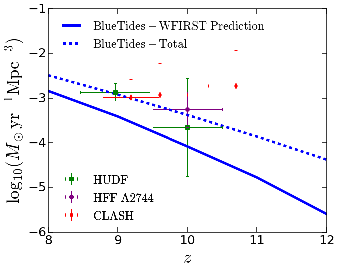
Figure 8: Star formation rate density prediction for the WFIRST HLS. The solid line shows the predicted result for WFIRST, without dust correction. The dashed line shows the contribution from the total BlueTides galaxy sample. Observational data points are for the HUDF (Oesch et al., 2014b), HFF A2744 (Oesch et al., 2015), and observational estimates from CLASH (Bouwens et al., 2014; Zheng et al., 2012; Coe et al., 2013)

Figure 8 shows the global star formation rate density prediction from BlueTides for galaxies in the WFIRST HLS, together with current observational constraints. It is important to note that the observational results are from galaxies with $M_{UV}<-18$ whereas at $z=8$, the WFIRST $5\sigma$ limit corresponds to $M_{UV}<-20.5$. This shows that galaxies fainter than this magnitude contribute $\sim 55$ per cent of the observed star formation rate density at $z=8$. By $z=12$, WFIRST will only be able to directly probe $\sim 6$ per cent of the total star formation rate density.

4.2 AGN Properties

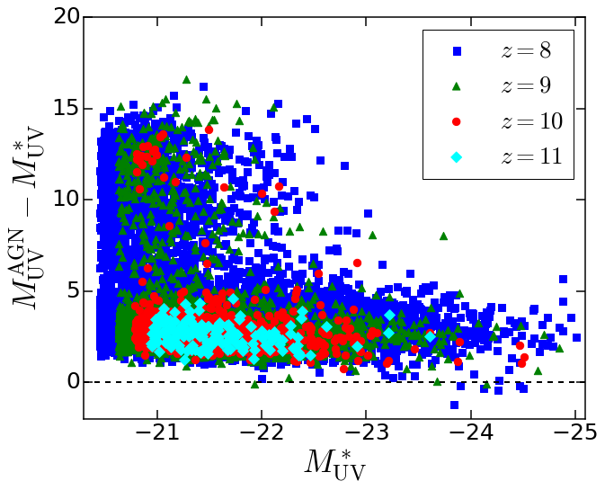
Figure 9: Magnitude difference of AGN and their host galaxies. Points below the dashed black line indicate AGN that out shine their host galaxy.

Figure 9 shows the relative brightness of AGN and their host galaxies for the WFIRST galaxy population. Only about 0.3 per cent of the AGN outshine their host galaxies at $z=8$ and $9$, while the rest of the AGN are $\gtrsim 1$ magnitude fainter than their host galaxy. These exceptionally bright black holes are those with the highest mass (see Di Matteo et al. (2016) in prep). By $z=10$, all of the AGN in the BlueTides volume are $\gtrsim 1$ magnitude fainter than their host galaxy.

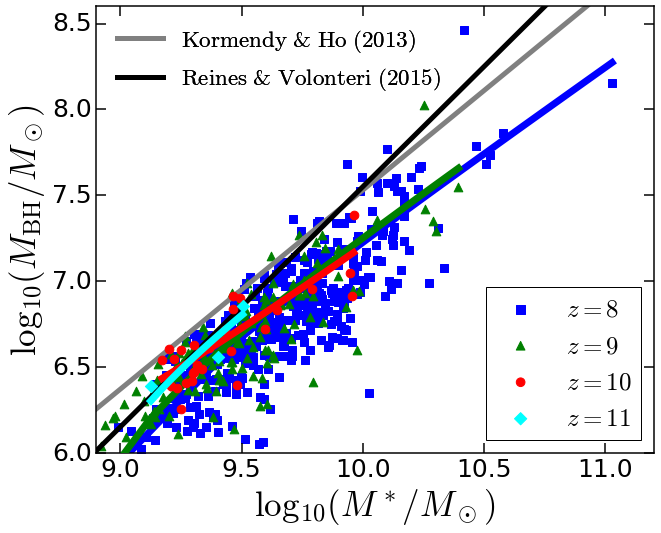
Figure 10: Black hole mass vs. stellar mass for the AGN brighter than the WFIRST $5\sigma$ limit. Data points show the distribution at each redshift. The solid lines show the best linear fit at each redshift. Grey and black lines show the best fits to local observations ($z<1$) from Kormendy & Ho (2013) and Reines & Volonteri (2015), respectively.

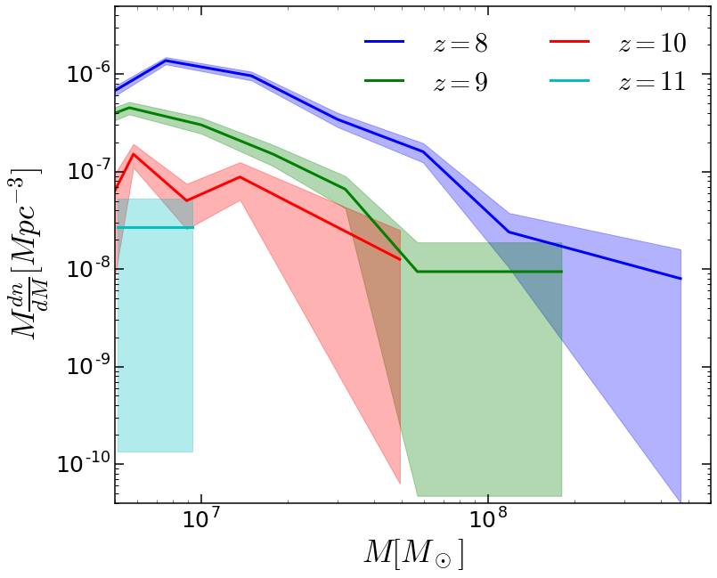
Figure 11: Black hole mass function for the AGN with intrinsic luminosities bright enough to be detected by WFIRST. Shaded region indicates $1\sigma$ Poisson errors.

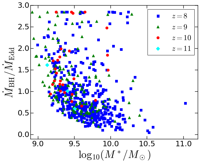
Figure 12: AGN mass accretion rate vs. stellar mass for the AGN with intrinsic luminosities bright enough to be detected by WFIRST.

Figure 10 shows black hole mass as a function of stellar mass, as well as a linear fit at each redshift. We find that for the AGN detectable by the WFIRST HLS, the $M_{\rm BH}/M^{*}$ ratio is about $2\times 10^{-3}$ at all redshifts, showing little redshift evolution. We show a comparison to local observations ($z<1$) from Kormendy & Ho (2013) and Reines & Volonteri (2015). Our high redshift results indicate a similar $M_{\rm BH}/M^{*}$ ratio to the local universe, but with about a $0.2$ dex offset in normalization. Figure 11 shows the black hole mass function (number density of black holes per unit mass) for the AGN brighter than the WFIRST $5\sigma$ cutoff. We see that the central super-massive black holes range in mass from $10^{6}-10^{8}h^{-1}M_{\odot}$. Figure 12 shows the ratio of the black hole mass accretion rate to its Eddington rate as a function of stellar mass. These AGN are accreting at a rate $\gtrsim 0.5\dot{M}_{\mathrm{edd}}$.

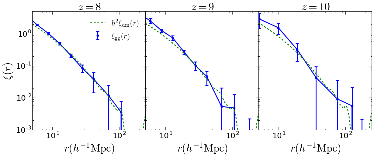
Figure 13: Galaxy correlation functions for redshifts $z=8,9,$ and $10$. Error bars are delete-one jacknife errors. Green dashed line shows the dark matter correlation function multiplied by the square of the linear bias.

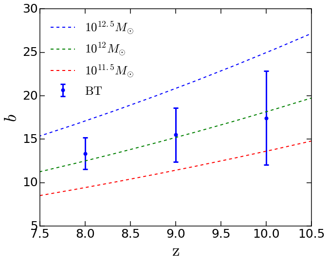
Figure 14: Bias measurements for the galaxies visible to WFIRST from BlueTides (blue points). Also shown is the linear bias computed from Tinker et al. (2010) for a given halo mass (dashed lines).

5 Clustering

Given the large sample of galaxies expected in the WFIRST HLS, it will be possible to measure their correlation functions at these high redshifts. Measurement of three-dimensional clustering will require galaxy redshift information. The WFIRST Grism survey is planned to cover about one third of the area of the HLS. It is designed primarily for searching for emission line galaxies with redshifts $z\approx 1-3$, using their H$\alpha$ lines and the OIII doublet. As a result the wavelength coverage is planned to be 1.35-1.89 microns with R=461. The galaxy described by Oesch et al. (2016) was confirmed to be at redshift $z=11.09$ from observation of the Ly$\alpha$ break in HST Grism spectroscopy. Given that we predict from BlueTides that large populations of galaxies of similar apparent magnitude exist at redshifts $z=8$, it is possible that redshifts can be measured to similar accuracy, depending on the performance of WFIRST spectroscopy. One obstacle to measuring redshifts below $z=10.1$ however is that the current lower limit of the WFIRST Grism coverage would exclude detection of the Ly$\alpha$ break.

Without spectroscopy, multiband photometric redshifts will be obtained for the galaxies we investigate in this work. For example, Calvi et al. (2016) have recently extended the BORG (Brightest of Reionizing Galaxies) survey to $z=9-10$ using HST five-band photometry. They find that approximately $30$ per cent of galaxies are interlopers with $z\sim 1$, whose Balmer break is masquerading as a Ly$\alpha$ break at higher z. This contamination results in a suppression in angular clustering which should be modeled. In this work, we concentrate on three dimensional measurements of the correlation function to illustrate the clustering bias and other properties of the galaxies in BlueTides. We leave specific modeling of the impact of Grism redshifts on three dimensional clustering (or projected clustering), and also angular clustering (for example using photometric information only) to future work. As a result, our speculations below on the possibility of detecting the BAO feature in clustering represent a best case scenario, intended to spur research into the idea of making a measurement at these high redshifts.

We calculate the correlation functions from the BlueTides galaxies as described in Section 2.3. We compute the correlation functions in real space, as we expect the redshift distortions of these highly biased objects to be small. To estimate errors on the galaxy correlation function, we utilize a delete-one jacknife method. We divide the BlueTides volume into eight sub samples and calculate the correlation function, removing each sub sample one at a time. The errors on the correlation function are then given by

$$\sigma^{2}(r)=\frac{N-1}{N}\sum_{i}^{N}(\xi(r)-\xi_{i}(r))^{2}$$ (7)

where $\xi(r)$ is the correlation function for the entire volume and $\xi_{i}(r)$ is the correlation function with the $i$th sub volume removed. Figure 13 shows the measured correlation function of the BlueTides  galaxies brighter than the WFIRST $5\sigma$ limit. Also shown is the dark matter correlation function. We multiply the dark matter correlation function by the bias computed in equation 4.

Barone-Nugent et al. (2014) measured a linear bias of $b=8.6$ using about 650 Lyman Break Galaxies at $z\sim 7$ in the HST Ultra Deep Fields. The WFIRST HLS will be capable of detecting $\sim 650$ galaxies at $z=13$ according to BlueTides. So WFIRST may have a large enough galaxy sample to determine the linear bias out to $z\sim 13$. The galaxy bias as a function of redshift is shown in Figure 14 with errors propagated forward from the jacknife errors on the galaxy correlation functions (no error assumed on the dark matter only correlation function). The WFIRST galaxy population in BlueTides implies values of $b=13.4\pm 1.8$ at $z=8$, which will be the largest bias ever measured. The galaxy bias increases linearly with redshift ($b\approx 2.1(1+z)-5.3$) reaching values close to $b\sim 20$ by $z=11$.

Figure 13 shows that at $r\sim 100h^{-1}$Mpc, the BlueTides galaxy correlation function is consistent with no BAO peak. This is a result of the relatively small simulation volume of BlueTides. However WFIRST HLS will cover a much bigger comoving volume (by a factor of $\sim 400$). The detectability of the BAO peak is largely determined by the survey volume and the product $nP_{\rm gg}$, where $n$ is the number density of the galaxy population and $P_{\rm gg}=b^{2}P_{\rm dm}$ is the galaxy power spectrum evaluated at the BAO scale $k=0.2h\rm Mpc^{-1}$. For $nP_{\rm gg}<1$, the error on the measurement of the BAO peak is dominated by shot noise. For $nP_{\rm gg}>1$ the BAO peak can be fully sampled for a strong detection. Given the bias measured above and the number density of galaxies in BlueTides (and the dark matter only power spectrum from Eisenstein & Hu (1998) for $P_{\rm dm}$) we can estimate the expected strength of the BAO signal.

	BOSS CMASS	WFIRST
$\bar{z}$	0.57	8.0
$z$	0.43 < z < 0.7	7.865 < z < 8.135
$P_{\text{dm}}(h^{-3}Mpc^{3})$	2040	75.3
$b$	2.0	13.36
$P_{\text{gg}}(h^{-3}Mpc^{3})$	8160	13240
$n\ (h^{3}Mpc^{-3})$	$3.0\times 10^{-4}$	$1.19-3.6\times 10^{-4}$
$nP_{\text{gg}}$	2.45	1.60-4.87
$A_{\text{Survey}}\ (\text{deg}^{2})$	3275	2200
$V\ (Gpc^{3})$	3.89	4.58

Table 2: Comparison of the BOSS CMASS sample (Anderson et al., 2012) and the WFIRST $z=8$ sample as predicted by BlueTides. $P_{\rm gg}$ and $P_{\rm dm}$ are computed at the BAO scale $k=0.2h/Mpc$ at the mean redshift of the sample in question. Ranges for $n$ (and $nP$) are computed using galaxies brighter than the WFIRST $5\sigma$ according to the intrinsic and dust corrected galaxy luminosities. $V$ is the comoving volume for each survey’s respective area coverage, assuming the same range in redshift centered about the mean redshift $\bar{z}$.

Table 2 shows the comparison at $z=8$ for BOSS CMASS (Anderson et al., 2012), which detected the BAO peak at the $5\sigma$ level, and WFIRST utilizing the number density and bias measurements from BlueTides. Although the dark matter power spectrum is an order of magnitude lower at $z=8$, we see that BlueTides predicts values of $nP_{\rm gg}$ for WFIRST at $z=8$ ($nP_{\rm gg}=1.60-4.87$ ) which are comparable to that of the BOSS CMASS sample ($nP_{\rm gg}=2.45$). This is due to the fact that the galaxy bias is larger by an order of magnitude and the expected number density at $z=8$ ($n=1.2-3.6\times 10^{-4}h^{3}{\rm Mpc}^{-3}$) is nearly the same as the BOSS CMASS number density ($n=3\times 10^{-4}h^{3}{\rm Mpc}^{-3}$). The comoving volume for WFIRST is shown in Table 2 for the same change in redshift as the BOSS CMASS sample, $\Delta z=0.27$, centered around $z=8$ to show that these surveys have similar observation volumes (before selection effects). Since the comoving volume of WFIRST is larger ($V=3.89{\rm Gpc}^{3}$ for BOSS CMASS and $V=4.58{\rm Gpc}^{3}$ for WFIRST), and the values of $nP_{\rm gg}$ are very comparable, this means that if sufficiently accurate redshift information was available for the galaxies, WFIRST would be able to detect the BAO signal at $z=8$. As we have noted above, in practice, the WFIRST Grism survey as planned will only cover one third of the area of the HLS, and its spectral coverage of the Lyman break will not include $z=8-9$ in any case. Our BAO predictions are therefore mostly illustrative, serving to highlight that there is potentially a large population of galaxies which could be used to make this cosmological measurement. Further work would be needed to decide whether changes to the WFIRST mission instrument parameters would be enough to make the measurement feasible.

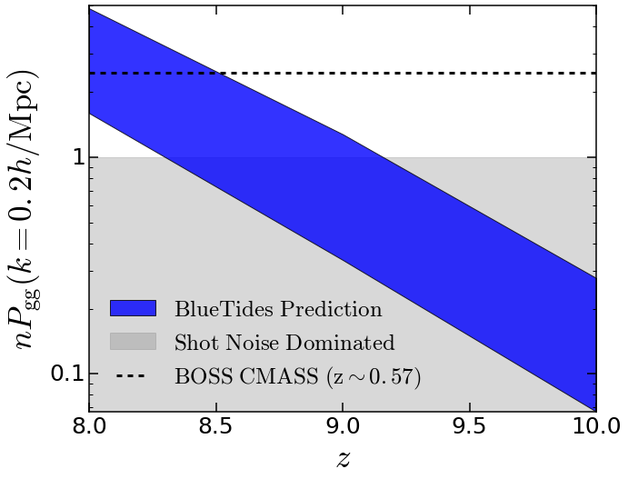
Figure 15: $nP_{\rm gg}$ computed for the WFIRST survey using the number density and bias computed from BlueTides. Upper (lower) limit uses the number density $n$ computed with the intrinsic (dust corrected) luminosities. Black line shows the value for the BOSS CMASS sample which detected the BAO peak at the $5\sigma$ level. (Anderson et al., 2012)

Figure 15 shows the product $nP_{\rm gg}$ at the BAO scale as a function of redshift. The blue band shows $nP_{\rm gg}$ for the number density of galaxies detectable by WFIRST determined by the intrinsic (upper limit) and dust corrected (lower limit) luminosities. The black dashed line shows $nP_{\rm gg}$ for the BOSS CMASS sample (Anderson et al., 2012). The error on the BAO measurement scales with $V_{\rm survey}^{-1/2}$ and $(1+nP_{\rm gg})/nP_{\rm gg}$ (Seo & Eisenstein, 2003). Using this as a rough measure for the detection strength of the BAO signal compared to the $5\sigma$ detection strength from the BOSS CMASS sample, BlueTides predicts a $\sim 4.7-6.3\sigma$ detection of the BAO signal at $z=8$. At $z=9$ and $z=10$, BlueTides predicts detection significances of $\sim 1.4-4.0\sigma$ and $\sim 0.5-1.5\sigma$, respectively, assuming accurate redshift information. We find a similar result following the method of Blake & Glazebrook (2003), including the effects of shot noise, so that the error on the power spectrum is given by $\sigma_{P}/P_{\rm gg}=2\pi(k^{2}\Delta kV_{\rm survey})^{-1/2}(1+nP_{\rm gg})/nP_{\rm gg}$. Assuming $\Delta k=0.015h/Mpc$, we find a $4.7\sigma$ difference between the galaxy power spectrum and the no-wiggle power spectrum of Eisenstein & Hu (1998) at the BAO scale for the non-dust corrected number density at $z=8$. We note again that inclusion of uncertainties on photometric redshifts, which will reduce the observed BAO signal, is necessary for a complete analysis.

6 Conclusions

Using the BlueTides cosmological hydrodynamic simulation, we have forecast the properties of the galaxy and AGN populations to be discovered by the WFIRST HLS in the redshift range $z=8-15$. The BlueTides simulation produces results which agree well with the galaxy LF from current HST observations, including the highest redshift galaxy to date (Oesch et al., 2016). Our conclusions for the BlueTides predictions are as follows:

• $\gtrsim 10^{6}$ star forming galaxies beyond $z=8$ will be detectable by the WFIRST HLS, significantly more than previously predicted (S13).

• We find that even with a dust-corrected model, the bright end of the luminosity function deviates from that of a standard Schechter function. This is relevant to the WFIRST LFs, since the HLS survey will only be able to detect the brightest galaxies at such high redshift.

• $z=15$ galaxies are likely to be within the $5\sigma$ detection limit of WFIRST  since dust effects seem to be small beyond $z=11$.

• Around $10^{4}$ AGN will have UV luminosities bright enough to be detected by WFIRST at $z=8$ and beyond. These will be the highest redshift AGN observed to date.

• The WFIRST galaxy population will have specific star formation rates of $\sim 10/{\rm Gyr}^{-1}$, ages between 10s to 100s of million years, and gas phase metallicities in the range $12+\log_{10}(O/H)=6{\rm\ to\ }8$. The galaxies will reside in dark matter halos with masses $\gtrsim 10^{10.5}M_{\odot}$.

• A few of the brightest AGN sources in the BlueTides volume outshine their host galaxy in the UV. The AGN WFIRST will observe have black hole masses that range from $10^{5}-10^{8}M_{\odot}$ and their mass accretion results in a luminosity around half the Eddington value or more.

• The WFIRST galaxy population will be very highly biased. The bias at $z=8$ will be $b=13.4\pm 1.8$ and will evolve linearly with redshift.

• Due to the high bias and large number density predicted by BlueTides, if redshift information is available for these galaxies (using the WFIRST Grism) WFIRST could perhaps detect the BAO peak to a high level of significance at $z=8$, comparable to that of the BOSS CMASS sample. We note that this would be unlikely as the mission is currently planned (requiring changes to the spectral coverage of the Grism). It is worth considering this result in the future, as it could lead to high redshift constraints on cosmological model parameters.

The WFIRST HLS will result in a huge change in our knowledge of the high redshift observational frontier. The number of observed galaxies will greatly increase: by the most conservative estimates derived from BlueTides, WFIRST will increase the $z=8-11$ galaxy sample by a factor of about 10,000 from the current sample and will observe the first galaxies at $z=12$ and beyond. The WFIRST observations will further constrain the epoch of reionization, galaxy formation theories, and cosmology in a new redshift regime.

7 Acknowledgements

We thank Sebastian Fromenteau for useful discussions. We acknowledge funding from NSF ACI-1036211, NSF AST-1517593, NSF AST-1009781, and the BlueWaters PAID program. The BlueTides simulation was run on facilities on BlueWaters at the National Center for Supercomputing Applications. SMW acknowledges support from the UK Science and Technology Facilities Council.

8 Appendix

8.1 DPL Fits to BlueTides LF

In Figure 16 we show the intrinsic luminosity functions for BlueTides galaxies with their best fit to the DPL defined in equation 5. Dust corrected luminosity functions are shown in Figure 17. We fit the DPL parameters’ redshift evolution assuming a linear evolution in $\log(\phi^{*}),M^{*},\alpha,{\rm and\ }\beta$. The results for the intrinsic LFs are:

$$\log(\phi^{*})=-\left[(0.96\pm 0.22)(z-8)+(2.54\pm 2.32)\right]$$

$$M^{*}=\left[(0.28\pm 0.12)(z-8)+(-24.51\pm 1.29)\right]$$ (8)

$$\alpha=-\left[(0.14\pm 0.02)(z-8)+(0.86\pm 0.22)\right]$$

$$\beta=-\left[(0.15\pm 0.05)(z-8)+(1.92\pm 0.55)\right]$$

and for the dust corrected LFs:

$$\log(\phi^{*})=-\left[(1.19\pm 0.06)(z-8)+(1.13\pm 0.62)\right]$$

$$M^{*}=\left[(0.03\pm 0.03)(z-8)+(-20.71\pm 0.32)\right]$$ (9)

$$\alpha=-\left[(0.16\pm 0.01)(z-8)+(0.66\pm 0.15)\right]$$

$$\beta=-\left[(0.22\pm 0.06)(z-8)+(2.42\pm 0.63)\right]$$

where $\phi^{*}$ is in $[{\rm Mpc}^{-3}{\rm mag}^{-1}]$.

We define the AGN power law LF as

$$\log(\phi)=\log(\phi^{*})+\log[0.4\log 10)]$$

$$+0.4\log(10)(M^{*}-M)(1-\alpha)$$ (10)

where we arbitrarily choose $M^{*}=-18.0$ (grey dashed lines in Figure 4). The best fit redshift evolutions are given by

$$\log(\phi^{*})=-\left[(1.44\pm 0.26)(z-8)+(26.15\pm 2.64)\right]$$

$$\alpha=-\left[(0.01\pm 0.07)(z-8)+(2.38\pm 0.68)\right]$$

(11)

8.2 Fits to Cumulative Number Density

The cumulative number of objects brighter than a given magnitude is well fit by a power law at each redshift (Figure 3). We fit the results with the following:

$$\log_{10}\left(N(<m_{\rm UV})/{\rm deg}^{2}\right)=A+b\ m_{\rm UV}$$ (12)

with

$$A=(-2.61\pm 0.22)(1+z)+(5.93\pm 2.83)$$ (13)

$$b=(0.07\pm 0.01)(1+z)+(0.19\pm 0.11)$$

for the intrinsic luminosities and

$$A=(-3.23\pm 0.29)(1+z)+(-1.74\pm 3.67)$$ (14)

$$b=(0.09\pm 0.01)(1+z)+(0.46\pm 0.14)$$

for the dust corrected luminosities.

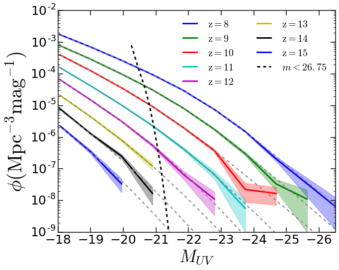
Figure 16: Intrinsic luminosity functions for BlueTides. Dashed lines show the best fit DPL defined in equation 5.

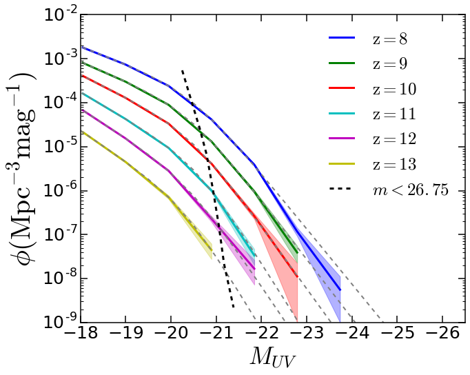
Figure 17: Dust corrected luminosity functions for BlueTides. Dashed lines show the best fit DPL defined in equation 5.

References

- Anderson et al. (2012) Anderson L., et al., 2012, MNRAS, 427, 3435
- Asplund et al. (2009) Asplund M., Grevesse N., Sauval A. J., Scott P., 2009, ARA&A, 47, 481