Detection, numerical simulation and approximate inversion of optoacoustic signals generated in multi-layered PVA hydrogel based tissue phantoms

Abstract

In this article we characterize optoacoustic signals generated from layered tissue phantoms via short laser pulses by experimental and numerical means. In particular, we consider the case where scattering is effectively negligible and the absorbed energy density follows Beer-Lambert’s law, i.e. is characterized by an exponential decay within the layers and discontinuities at interfaces. We complement experiments on samples with multiple layers, where the material properties are known a priori, with numerical calculations for a pointlike detector, tailored to suit our experimental setup. Experimentally, we characterize the acoustic signal observed by a piezoelectric detector in the acoustic far-field in backward mode and we discuss the implication of acoustic diffraction on our measurements. We further attempt an inversion of an OA signal in the far-field approximation.

1 Introduction

Recent progress in the field of optoacoustics (OAs) has been driven by tomography and imaging applications in the context of biomedical optics. Motivated by their immediate relevance for medical applications, high resolution scans on living tissue proved the potential of the optical absorption based measurement technique [1, 2, 3]. Requiring a multitude of detection points around the source volume, OA tomography allows for the reconstruction of highly detailed images, see, e.g., Ref. [4], assuming a mathematical model that mediates the underlying diffraction transformation of OA signals in the forward direction [5, 6, 7, 8].

However, for most cases of in vivo measurements, especially on humans, it is not feasible to place ultrasound detectors in opposition to the illumination source (with the “object” in between), i.e. to work in forward mode. Instead, it is worked in backward mode, where detector and irradiation source are positioned on the same side of the sample. Using elaborate setups combining the paths of light and sound waves it is possible to co-align optical and acoustic focus within the sample. By scanning over a multitude of detection points it is then possible to produce $3$D images with very high resolution, see, e.g., Ref. [9].

A conceptually different approach is to perform measurements by means of a single, unfocused transducer. Albeit it is not possible to reconstruct OA properties of arbitrary $3$D objects with a fixed irradiation source and a single detection point only, useful information of the internal material properties of, say, layered samples can be gained nevertheless. In this regard, acoustic near-field measurements by means of a transparent optoacoustic detector where shown to reproduce the depth profile of absorbed energy density and absorption coefficient without the need of extensive postprocessing [10, 11, 12, 13]. However, requiring close proximity and plane wave symmetry, near-field conditions are unrealistic considering most measurement scenarios. In contrast, the acoustic far-field regime allows for a much higher experimental flexibility, although at the cost of the straight forward interpretation of the measurements. More precisely, in the far-field, when the distance between detector and source is large compared to the lateral extend of the source, OA signals exhibit a diffraction-transformation which is characteristic for the underlying system parameters [14, 15, 16, 17]. In particular, in the acoustic far-field, OA signals exhibit a train of compression and rarefaction peaks and phases, signaling a sudden change of the absorptive characteristics of the underlying layered structure.

In the presented article we thoroughly prepare and analyze polyvinyl alcohol hydrogel (PVA-H) phantoms, comprised of layers doped with different concentrations of melanin. The acoustic properties of the PVA-Hs match those of soft tissue, i.e. human skin [18, 19]. Note that melanin is the main endogenous absorber in the epidermis [20], and, more importantly, in melanomas. Layers with higher concentrations of melanin absorb a greater amount photothermal energy and expand more intensely than surrounding layers with low concentrations. The stress waves emitted by these OA sources, detected in the acoustic far field after experiencing a shape transformation due to diffraction, are put under scrutiny here. Therefore, experimental measurements are complemented by custom numerical simulations. Besides analytic theory and experiment, the latter form a “third pillar” of contemporary optoacoustic studies [5].

The paper is organized as follows. In Sec. 2 we recap the theoretical background of optoacoustic signal generation and detail our numerical approach to compute the respective signals for point-detectors. In Sec. 3 we describe our experimental setup and elaborate on the preparation of the tissue phantoms used for our measurements, followed by details of the experiments and complementing simulations in in Sec. 4. We summarize our findings in Sec. 5.

2 Theory and numerical implementation

We briefly recap the general theory of optoacoustic signal generation in Subsec. 2.1. Subsequently, in Subsec. 2.2, we customize the general optoacoustic poisson integral to properly represent the layered tissue phantoms and irradiation source profile used in our experiments. Finally, in Subsec. 2.3, we emphasize some important implications of the problem-inherent symmetries on our numerical implementation.

2.1 General optoacoustic signal generation

In thermal confinement, i.e. considering short laser pulses with pulse duration significantly smaller than the thermal relaxation time of the underlying material [8, 21], the inhomogeneous optoacoustic wave equation relating the scalar pressure field $p(\vec{r},t)$ to a heat absorption field $H(\vec{r},t)$ reads

$$\Big{[}\partial_{t}^{2}-c^{2}\vec{\nabla}^{2}\Big{]}~{}p(\vec{r},t)=\partial_{t}~{}\Gamma H(\vec{r},t).$$ (1)

Therein, $c$ signifies the speed of sound and $\Gamma$ refers to the Grüneisen parameter, an effective parameter summarizing various macroscopic material constants, describing the fraction of absorbed heat that is actually converted to acoustic pressure. As evident from Eq. (1), temporal changes of the local heat absorption field serve as sources for stress waves that form the optoacoustic signal. Following the common framework of stress confinement [5], we consider a product ansatz for the heating function in the form

$$H(\vec{r},t)~{}=~{}W(\vec{r})\delta(t),$$ (2)

where $W(\vec{r})$ represents the volumetric energy density deposited in the irradiated region due to photothermal heating by a laser pulse [22], which, on the scale of typical acoustic propagation times, is assumed short enough to be represented by a delta-function. Consequently, an analytic solution for the optoacoustic pressure at the field point $\vec{r}$ can be obtained from the corresponding Greens-function in free space, yielding the optoacoustic Poisson integral [23, 24, 25]

$$p(\vec{r},t)=\frac{\Gamma}{4\pi c}\partial_{t}\int\limits_{V}\!\frac{W(\vec{r}^{\prime})}{|\vec{r}-\vec{r}^{\prime}|}\delta(|\vec{r}-\vec{r}^{\prime}|-ct)\,\mathrm{d}\vec{r}^{\prime},$$ (3)

where $V$ denotes the “source volume” beyond which $W(\vec{r}^{\prime})=0$ [26], and $\delta(\cdot)$ limiting the integration to a time-dependent surface constraint by $|\vec{r}-\vec{r}^{\prime}|=ct$.

2.2 The Poisson integral for layered media in cylindrical coordinates

As pointed out earlier, we consider non-scattering compounds, composed of (possibly) multiple plane-parallel layers, stacked along the $z$-direction of an associated coordinate system. Whereas the acoustic properties are assumed to be constant within the medium, the optical properties within the absorbing medium might change from layer to layer. Thus, the volumetric energy density naturally factors according to

$$W(\vec{r})~{}=~{}f_{0}f(x,y)g(z),$$ (4)

wherein $f_{0}$ signifies the energy fluence of the incident laser beam on the $z=0$ surface of the absorbing material, and $f(x,y)$ and $g(z)$ specify the two-dimensional ($2$D) irradiation source profile and the $1$D axial absorption depth profile, respectively. Bearing in mind that we consider non-scattering media, the latter follows Beer-Lambert’s law, i.e.

$$g(z)=\mu_{\rm a}(z)\exp\Big{\{}-\int_{0}^{z}\!\mu_{\rm a}(z^{\prime})\,\mathrm{d}z^{\prime}\Big{\}},$$ (5)

wherein $\mu_{\rm a}(z)$ denotes the depth-dependent absorption coefficient.

Note that, for a plane-normal irradiation source with an axial symmetry, there are two useful auxiliary reference frames based on cylindrical polar coordinates: (i) $\Sigma_{\rm I}$ where $\vec{r}=\vec{r}(\rho,\phi,z)$ with origin on the beam axis at the surface of the absorbing medium, and, (ii) $\Sigma_{\rm D}$ where $\vec{r}^{\prime}=\vec{r}^{\prime}(\rho^{\prime},\phi^{\prime},z^{\prime})$ with origin at the detection point $\vec{r}_{\rm D}=(x_{\rm D},0,z_{\rm D})$ in $\Sigma_{\rm I}$, see Fig. 1. Both reference frames are related by the point transformation $\vec{r}^{\prime}(\rho^{\prime},\phi^{\prime},z^{\prime})=\vec{r}-\vec{r}_{\rm D}$ [27].

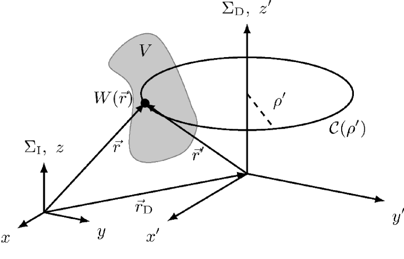
Figure 1: Illustration of the two reference frames $\Sigma_{\rm I}$, with origin on the beam axis at the surface of the absorbing medium, and, $\Sigma_{\rm D}$ with origin right at the detection point. Both coordinate systems are related by the transformation $\vec{r}^{\prime}(\rho^{\prime},\phi^{\prime},z^{\prime})=\vec{r}-\vec{r}_{\rm D}$ [27]. Considering cylindrical polar coordinates in $\Sigma_{\rm D}$ allows to factor the volumetric energy density $W(\vec{r})$ within the source volume $V$ as detailed in the text and to pre-compute the contribution of the irradiation source profile along closed polar curves $\mathcal{C}(\rho^{\prime})$ with radius $\rho^{\prime}$. This in turn yields an efficient numerical scheme to compute the optoacoustic signal $p_{\rm D}(t)$ at the detection point $\vec{r}_{\rm D}$.

In $\Sigma_{\rm I}$ the irradiation source profile takes the convenient form $f(x(\rho,\phi),y(\rho,\phi))\equiv f_{\rm I}(\rho)$, where beam-profiling measurements for our experimental setup are consistent with a top-hat shape

$$f_{\rm I}(\rho)=\begin{cases}1,&\text{if }\rho\leq a\\ \exp\{-(\rho-a)^{2}/d^{2}\},&\text{if }\rho>a\end{cases}.$$ (6)

In $\Sigma_{\rm D}$ the constituents of the volumetric energy density read $f_{\rm D}(\rho^{\prime},\phi^{\prime})\equiv f(x_{\rm D}+\rho^{\prime}\cos(\phi^{\prime}),\rho^{\prime}\sin(\phi^{\prime}))$ and $g_{\rm D}(z)\equiv g(z^{\prime}-z_{\rm D})$, so that the optoacoustic Poisson integral, i.e. Eq. (3), takes the form

$$p_{\rm D}(t)=\frac{f_{0}\Gamma}{4\pi c}\partial_{t}\iiint\limits_{V}\!\rho\frac{f_{\rm D}(\rho,\phi)g_{\rm D}(z)}{(\rho^{2}+z^{2})^{1/2}}\\ \times\delta((\rho^{2}+z^{2})^{1/2}-ct)\,\mathrm{d}\rho\,\mathrm{d}\phi\,\mathrm{d}z.$$ (7)

Albeit the non-canonical formulation of the Poisson integral in cylindrical polar coordinates might seem a bit counterintuitive at first, it paves the way for an efficient numerical algorithm for the calculation of optoacoustic signals for layered media.

2.3 Numerical experiments

Implementation details

Considering a partitioning of the radial coordinate into $N_{\rho}$ equal sized values $\Delta\rho=L_{\rho}/N_{\rho}$ so that $\rho_{i}=i\Delta\rho$ with $i=0\ldots N_{\rho}-1$, the preceding factorization of the volumetric energy density $W(\vec{r})$ in $\Sigma_{\rm D}$ allows to pre-compute the contribution of the irradiation source profile in Eq. (7) along closed polar curves $\mathcal{C}(\rho_{i})$ with radius $\rho_{i}$ according to

$$F_{\rm D}(\rho_{i})=\lim_{N_{\phi}\to\infty}\rho_{i}\sum_{j=0}^{N_{\phi}-1}f_{\rm D}(\rho_{i},\phi_{j})~{}\Delta\phi,$$ (8)

where $\Delta\phi=2\pi/N_{\phi}$ and $\phi_{j}=j\Delta\phi$ with $j=0\ldots N_{\phi}-1$, thus completing the integration over the azimuthal angle and providing the results in a tabulated manner with time complexity $O(N_{\rho}N_{\phi})$. This in turn yields an efficient numerical scheme to compute the optoacoustic signal $p_{\rm D}(t)$ at the detection point $\vec{r}_{\rm D}$ since the pending integrations can, in a discretized setting with $\Delta z=L_{z}/N_{z}$ so that $z_{k}=k\Delta z$ for $k=0\ldots N_{z}-1$, be carried out with time complexity $O(N_{\rho}N_{z})$. Consequently, interpreting the $\delta$-distribution in Eq. (7) as an indicator function that bins the values of the integrand according to the propagation time of the associated stress waves, the overall algorithm completes in time $O(N_{\rho}N_{\phi}+N_{\rho}N_{z})$. Note that for the special case $x_{\rm D}=y_{\rm D}=0$, i.e. for detection points on the beam axis, Eq. (8) further simplifies to $F_{\rm D}(\rho_{i})=2\pi\rho_{i}f_{\rm I}(\rho_{i})$, reducing the time complexity to only $O(N_{\rho}N_{z})$ [28]. During our numerical simulations , for practical purposes and since we are only interested in the general shape of the optoacoustic signal in order to compare them to the transducer response, we set the value of the constants in Eq. (7) to $f_{0}\Gamma/c\equiv 4\pi$. Thus, the resulting signal is obtained in arbitrary units, subsequently abbreviated as $[{\rm a.u.}]$, making it necessary to adjust the amplitude of the signal if we intent to compare the results to actual measurements. Further, to mimic the finite thickness $\Delta w$ of the transducer foil, see Sec. 3, we averaged the optoacoustic signal at the detection point over a time interval $\Delta t=\Delta w/c$.

Exemplary optoacoustic signals

So as to facilitate intuition and to display the equivalence of the numerical schemes implemented according to Eqs. (3) and (7) in both, the acoustic near field (NF) and far field (FF), we illustrate typical optoacoustic signals in Fig. 2. Therein, the “cartesian” solver was based on a voxelized cubic representation of the source volume with side-lengths $(L_{x},L_{y},L_{z})=(0.6,0.6,0.15)~{}[{\rm cm}]$ using $(N_{x},N_{y},N_{z})=(1500,1500,150)$ meshpoints, whereas the solver based on cylindrical coordinates used a decomposition of the computational domain into $(L_{\rho},L_{z})=(0.3,0.15)~{}{\rm cm}$ and $(N_{\rho},N_{\phi},N_{z})=(6000,360,150)$. The parameters defining the irradiation source profile were set to $a=0.15~{}{\rm cm}$ and $d=a/4$. As finite thickness of the transducer foil we considered $\Delta w=50~{}{\rm\mu m}$ in both setups.

The dimensionless diffraction parameter $D=2|z_{\rm D}|/(\mu a_{0}^{2})$ [14, 12] can be used to distinguish the acoustic near field (NF) at $D<1$ and far field (FF) at $D>1$. Here, we consider the effective parameters $\mu=\langle\mu_{\rm a}(z)\rangle$ and $a_{0}=1.25\cdot a$ in case of multi-layered tissue phantoms. The simulations were performed at detection points on the beam axis, realizing NF conditions with $D\approx 0.15$ at $z_{\rm D}=-0.04~{}{\rm cm}$ and FF conditions with $D\approx 15.0$ at $z_{\rm D}=-4.0~{}{\rm cm}$. As evident from Fig. 2, the optoacoustic NF signals are characterized by an extended compression phase in the range $c\tau=0.0-0.1~{}{\rm cm}$, originating from the plane-wave part of the propagating stress wave and accurately tracing the profile of the volumetric energy density along the beam axis, followed by a pronounced diffraction valley for $c\tau>0.11~{}{\rm cm}$. The particular shape of the latter is characteristic for the top-hat irradiation source profile used for the numeric experiments. In contrast to this, as can be seen from Fig. 2, the FF signal features a succession of compression and rarefaction phases. Therein a sudden increase (decrease) of the absorption coefficient is signaled by a compression peak (rarefaction dip), cf. the sequence of peaks and dips at the points $c\tau=0,~{}0.05,~{}0.10~{}{\rm cm}$ in Figs. 2(a,b). Further, the diffraction valley has caught up, forming rather shallow rarefaction phases in between the peaks and dips [30]. Finally, note the excellent agreement of the signals obtained by the two independent OA forward solvers.

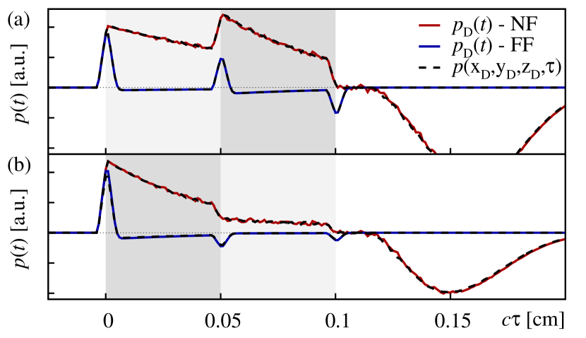
Figure 2: (Color online) Comparison of different solvers for the optoacoustic problem for layered media. The data curves labeled by $p_{\rm D}(t)$ refer to an implementation in cylindrical polar coordinates according to Eq. 7. The curves are computed for a field point in the acoustic near-field (NF; red line) and far-field (FF; blue line) at $z_{\rm D}=-0.04~{}{\rm cm}$ and $z_{\rm D}=-4.0~{}{\rm cm}$ on the beam axis, respectively. The corresponding numerical results obtained using an implementation of Eq. 3 in Cartesian coordinates are labeled by $p(\vec{r}_{\rm D},\tau)$ (black dashed lines). (a) Setup where the source-volume encloses two absorbing layers consisting of $\mu_{a}=10~{}\rm{cm^{-1}}$ in the range $z=0.0-0.05~{}{\rm cm}$ (light-gray shaded region) followed by $\mu_{a}=20~{}\rm{cm^{-1}}$ in the range $z=0.05-0.1~{}{\rm cm}$ (gray shaded region), and, (b) setup where the order of the layers is reversed.

In a second series of simulations we clarified the influence of the radial deviation of the detection point $\vec{r}_{\rm D}$ from the beam axis. Therefore we computed the excess pressure $p_{\rm D}(t)$ at different positions $x_{\rm D}\neq 0$ perceived in $\Sigma_{\rm I}$. The results for $x_{\rm D}=0.1~{}{\rm cm}$, i.e. 2/3 along the flat-top part of the top-hat profile, and $x_{\rm D}=0.2~{}{\rm cm}$, i.e. slightly above the $1/e$-width of the beam intensity profile, are illustrated in Fig. 3. As evident from Fig. 3(a), for $z_{\rm D}=-0.2~{}{\rm cm}$, realizing a location with $D=0.76$ in the acoustic NF, the optoacoustic signal appears to be quite sensitive to the precise choice of $x_{\rm D}$. I.e., as soon as the border of the plane-wave part of the signal is approached, the transformation of the signal due to diffraction is strongly visible. Comparing the points $z_{\rm D}=-1.0~{}{\rm cm}$ ($D=11.4$) in the “early” FF and $z_{\rm D}=-5.0~{}{\rm cm}$ ($D=19.0$) in the “deep” FF, it is apparent that the optoacoustic signal in the FF is less influenced by the off-axis deviation of the detection point, see Figs. 3(b,c). Also, note that with increasing distance $|z_{\rm D}|$, the interjacent rarefaction phases level off and move closer to the leading compression peaks [30]. From the above we conclude that, if we complement actual measurements recorded in the FF via numerical simulations, we should find a good agreement between detected and calculated signals even though both exhibit different degrees of deviation from the beam axis.

This completes the discussion of optoacoustic signals and their generation from a point of view of computational theoretical physics. Details regarding the optoacoustic detection device and the tissue phantoms are given in the subsequent section.

3 Methods and Material

Photoacoustic measurement setup

In the following, the experimental setup is presented with focus on the phantom preparation process and arrangement of the layered tissue samples [31]. For the detection of the OA pressure transient a self-built piezoelectric transducer is employed. This ultrasound detector comprises a $9\text{\,}\mathrm{\SIUnitSymbolMicro m}$ thick piezoelectric polyvinylidenfluorid (PVDF) film on both sides of which $\sim$$50\text{\,}\mathrm{n}\mathrm{m}$ indium tin oxide (ITO) electrodes are sputtered [11]. The active area of the detector is circular with a diameter of $1\text{\,}\mathrm{mm}$. As acoustic backing layer a piece of hydrogel was prepared and placed on top of the detector with a drop of distilled water to ensure acoustic coupling. Due to identical acoustic impedances of the backing layer and the phantom in addition to the marginal extent of the PVDF film in comparison to the acoustic wavelengths, the detector can be seen as acoustically transparent [10].

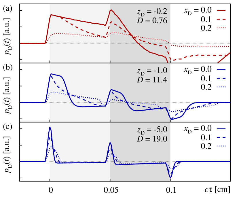
Figure 3: (Color online) Sensitivity of the optoacoustic signal $p_{\rm D}(t)$ on a radial deviation of the detection point $\vec{r}_{\rm D}$ from the beam axis, realized by setting $x_{\rm D}\neq 0~{}{\rm cm}$, as explained in the text. The subfigures refer to different distances $z_{\rm D}$, where (a) $z_{\rm D}=-0.2~{}{\rm cm}$ is located in the acoustic NF with $D=0.76$, (b) $z_{\rm D}=-1.0~{}{\rm cm}$ ($D=11.4$) in the “early” FF, and, (c) $z_{\rm D}=-5.0~{}{\rm cm}$ ($D=19.0$) in the “deep” FF.

In contrast to the numerical approach followed in the preceding section, the irradiation in our experimental setup had to be adjusted to an angle approximately $20\text{\,}\mathrm{\SIUnitSymbolDegree}$ off the plane normal, with the light entering the phantom in close proximity of the detector, see Fig.4. As laser source, an optical parametric oscillator (NL303G + PG122UV, Ekspla, Lithuania) at a wavelength of $532\text{\,}\mathrm{nm}$ is coupled into a $800\text{\,}\mathrm{\SIUnitSymbolMicro m}$ fiber (Ceramoptec, Optran WF 800/880N). The pulse duration from the pump is 3-$6\text{\,}\mathrm{n}\mathrm{s}$. The beam profile measured after the fiber is in good agreement with a top-hat shape, which is in accordance with the irradiation source profile Eq. (6), considered for the previous numerical experiments, and parameters as detailed for the numerical simulations in Sec. 4.

To improve the signal-to-noise ratio and match the electrical impedance, a custom build electrical pre-amplifier is connected to the detector electrodes. The voltages, corresponding to the detected pressure, are recorded at 2 GSPS (Giga sample per second) by a high-speed data acquisition card (Agilent U1065A, up to 8GSPS). At such sampling rates, the expected ultrasound pressure profile is highly over-sampled, thus, the point to point noise can be smoothed out without loss of information. A conservative estimation of the fastest changing signal features yield a time window of $20\text{\,}\mathrm{n}\mathrm{s}$ over which smoothing might be carried out, corresponding to 40 consecutive data points.

Polyvinyl alcohol based hydrogel tissue phantom recipe

The tissue phantoms used in our studies are compounds composed of stacked layers of polyvinyl alcohol hydrogel (PVA-H)[32]. The incentive to utilize PVA-H is its acoustic similarity to soft tissue, i.e. human skin [18]. In contrast to liquid phantoms such as water ink solutions [12], hydrogels have the advantage of being stackable without the need of containing walls. Furthermore, while liquids would intermix at interfaces and thus require solid boundaries in between, hydrogels allow sharp junctions only softened by diffusion. In the remainder the phantom creation recipe is detailed.

Here, PVA-Hs are produced by mixing polyvinyl alcohol granulate (Sigma-Aldrich 363146, Mw 85-124 99+% hydrolyzed) with distilled water at a mixing ratio 1:5. Using a magnetic stirrer with heating, the dispersion is kept at $94\text{\,}\mathrm{\SIUnitSymbolCelsius}$ for at least $40\text{\,}\mathrm{m}\mathrm{i}\mathrm{n}\mathrm{u}\mathrm{t}\mathrm{e}\mathrm{s}$ while the stirring bar rotates at $350\text{\,}\mathrm{R}\mathrm{P}\mathrm{M}$, until it becomes a homogeneous solution. This viscous mass can be poured into any mold to obtain the desired form. Depending on the required thickness, a commercial metal spacing washer or a 3D printed plastic ring of specific height was placed in between two glass plates, thus creating very flat PVA-H cylinders. Due to the much larger lateral extend of the phantoms, compared to the depth of the absorbing layers, boundary effects do not interfere with the optoacoustic signal.
To facilitate polymerization the phantom is subjected to one freezing and thawing cycle. The phantom is placed in the freezer at $-14\text{\,}\mathrm{\SIUnitSymbolCelsius}$ for $2\text{\,}\mathrm{d}\mathrm{a}\mathrm{y}\mathrm{s}$. Thawing is achieved by keeping the samples at room temperature for a few minutes, afterwards the phantoms are ready to use. Crystallites produced by freezing of water in the hydrogels would yield turbidity [33]. As a remedy, so as to obtain clear PVA-H, water soluble anti freezing agents are added. Here, when the PVA is completely dissolved, $\sim$$45\text{\,}\mathrm{v}\mathrm{o}\mathrm{l}\mathrm{\char 37\relax}$ pure ethanol was added to the aqueous solution incrementally, each time waiting for the schlieren to dissolve. Especially after adding the ethanol it is very important to keep the vessel closed whenever possible.

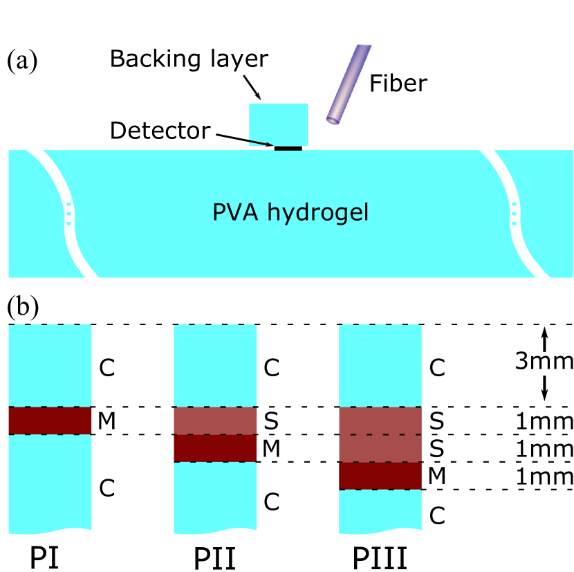
Figure 4: (Color online) Sketch of the experimental setup. (a) Arrangement of the components as discussed in the text, see sec. 3. (b) Layer composition of the three different phantoms PI, PII and PIII used for our measurements and the numerical simulations reported in sec. 4. The label “C” represents clear PVA-H, “S” labels low absorption, and “M” stands for high absorption. Note that, the clear layer at the bottom is $10\text{\,}\mathrm{mm}$ thick. Thus, signal reflections from interfaces of materials with differing acoustic properties occur well outside the measurement range in that direction.

The optical properties of the samples can be manipulated by inclusion of scatterers and or absorbers. In our studies, synthetic melanin (Sigma-Aldrich, M0418-100MG) was chosen as absorber to mimic melanoma, that is, black skin cancer. Due to its robustness to temperature, the finely ground melanin can be included in the beginning of the phantom creation process, at the same time with the PVA pellets. As a rough estimate it is assumed that melanomas contain as much melanin as African skin. According to [34], dark skin contains 10 times the melanin as compared to very fair skin, not taking into account the type of melanin. So as to reproduce the contrast of a melanoma in Caucasian skin the following different types of PVA-H layers were created:

• PVA-H without melanin, referred to as “C”,

• PVA-H with $1\text{\,}\mathrm{mg}\text{/}\mathrm{mL}$ of melanin, referred to as “M”, and,

• PVA-H with $0.1\text{\,}\mathrm{mg}\text{/}\mathrm{mL}$ of melanin, referred to as “S”,

By stacking these in different order, three distinct phantoms were created, see Fig. 4. Note that, the melanin concentrations specified above relate to the amount of hydrogel before the addition of ethanol. In the presented study we considered non-scattering material only, thus we did not add any scattering supplements.

Further hints for handling the tissue phantoms

Below we list practical hints and findings which proved very helpful in the course of tissue phantom production:

• In a closed screw neck bottle the aqueous solution can be stored for weeks at room temperature. However, note that after the flask has been reheated and opened several times, inevitable ethanol evaporation might cause turbidity upon freezing.

• The undesirable formation of bubbles within the phantoms can be avoided, to a great extend, by overfilling the spacing ring and mounting the top glass plate on the sample after the hydrogel has settled for a while. This procedure prohibits trapping of air at the spacing ring boundaries as well as giving the hydrogel some time to degas.

• While stacking the PVA-H layers in preparation for a measurement, the individual phantom layers should be kept wet by means of distilled water in order to prevent them from sicking together with one another and, most of all, themselves. Also, a proper watery film prohibits the inclusion of air in between layers.

4 Results

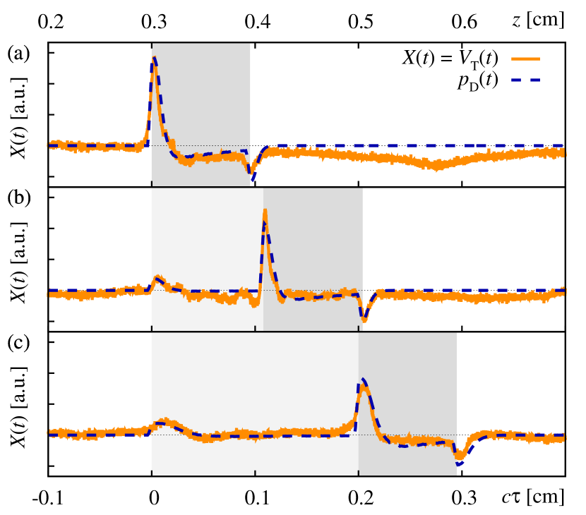
Figure 5: (Color online) Comparison of optoacoustic signals for layered media obtained from measurements ( labeled “$V_{\rm D}(t)$”; orange solid lines) and numerical simulations (labeled “$p_{\rm D}(t)$”; blue dashed lines). The top and bottom abscissas refer to the distance $z$ traveled by the signal and the retarded signal depth $c\tau=ct-z_{\rm D}$ (where $z_{\rm D}=0.3~{}{\rm cm}$), respectively. (a) single-layer tissue phantom ${\rm PI}$, (b) double-layer tissue phantom ${\rm PII}$, and, (c) double-layer tissue phantom ${\rm PIII}$, see Fig. 4(b). The layer with different melanin concentrations are indicated by the light-gray (in case of “S”; cf. 4(b)) and gray (in case of “M”; cf. 4(b)) shaded regions. Note, the presented data was obtained in single measurement and was neither smoothed nor averaged.

Below we complement measured PA signals, obtained from measurements on the three tissue phantoms ${\rm PI-III}$, discussed in Sec. 3 and illustrated in Fig. 4(b), with custom simulations obtained in terms of the numerical framework detailed in Sec. 2. As evident from the comparison of the experimental setup with the simulation framework, there are three distinctions between experiment and theory which have to be kept in mind while interpreting the results: (i) while the irradiation source is assumed to be plain normal incident for our simulations, the direction of incidence in the experimental setup exhibits a nonzero angle off the plane normal. Additionally, due to unavoidable refraction at the phantom surface, the beam profile is likely to be non-symmetric and slightly divergent. Hence, the top-hat beam shape assumed in our simulation approach can only been seen as an approximation of the experimental conditions. (ii) although it is probable that all the measurements are performed, at least to some extend, off-axis we opt for modeling and numerical simulations in an on-axis approach. As demonstrated in Subsec. 2.3 and illustrated in Fig. 3(c), we expect the principal signal shape in the acoustic far-field to change only at a small rate upon deviation from the beam axis. (iii) as pointed out in sec. 3, the active area of the transducer has a radius of $0.5~{}{\rm mm}$, while in our simulations we compute optoacoustic signals for a pointlike detector. However, upon approaching the far-field limit one expects the former intrinsic length scale not to be of significance. Albeit we plan to address this issue in future work, the apparent qualitative agreement of simulation and experiment detailed in the remainder is impressive and should suffice to validate our approach.

Comparison of optoacoustic signals obtained in theory and experiment

The measured optoacoustic signals for the tissue phantoms ${\rm PI-III}$ along with the simulated curves are illustrated in Figs. 5(a-c). In principle all three measured curves exhibit the characteristic features expected for signals observed in the acoustic far-field. Thus these measurements are well suited for the purpose of optoacoustic depth profiling [12]. In particular, for the simulation of ${\rm PI}$ we considered a single layer with absorption coefficient $\mu_{a}=11~{}{\rm cm^{-1}}$ in the range $z=0.3-0.395~{}{\rm cm}$ (note that $z$ is measured with respect to the origin of $\Sigma_{\rm D}$), indicated by a gray shaded region representing a highly absorbing layer (introduced as “M” in sect. 3). The top-hat beam shape parameters within the simulation where set to $a=0.054~{}{\rm cm}$ and $R\equiv d/a=1.5$. Note that both principal features of the signal, i.e. the initial compression peak as well as the trailing rarefaction dip are reproduced well and the intermediate rarefaction phase matches well in theory and experiment. The subsequent long and shallow rarefaction phase for $z>0.5~{}{\rm cm}$ is located outside the measurement range that corresponds to the prepared source volume and is likely caused by acoustic reflections from the lateral boundaries of the backing layer.

The same holds for the analysis of the remaining two phantoms, where ${\rm PII}$ was modeled by considering a first layer with a comparatively low absorption coefficient $\mu_{a}=1.4~{}{\rm cm^{-1}}$, i.e. type-S, in the range $z=0.3-0.408~{}{\rm cm}$ (light-gray shaded region), followed by a type-M layer with $\mu_{a}=11~{}{\rm cm^{-1}}$ in the range $z=0.408-0.504~{}{\rm cm}$ (gray shaded region). Therein, the beam shape parameters where set to $a=0.056~{}{\rm cm}$ and $R=1.2$. Here, all three expected characteristic signal features, i.e. the initial small compression peak, the interjacent high compression peak as well as the trailing rarefaction dip match well for theory and experiment.

Finally, phantom ${\rm PIII}$ was modeled by considering a type-S layer with $\mu_{a}=1.4~{}{\rm cm^{-1}}$ in the range $z=0.3-0.5~{}{\rm cm}$ (light-gray shaded region) followed by a type-M layer with $\mu_{a}=11~{}{\rm cm^{-1}}$ in the range $z=0.5-0.595~{}{\rm cm}$ (gray shaded region). Therein, the beam shape parameters where set to $a=0.08~{}{\rm cm}$ and $R=1.2$. Again, all three characteristic signal features are reproduced well by theory and experiment.

Note that, as pointed out in subsec. 2.3, it is necessary to adjust the scale of the amplitude of the computed PA signal if we intend to compare it to the transducer response. The respective scaling factor was obtained from the simulated and measured curves for tissue phantom ${\rm PI}$ and was subsequently used in the other two cases to achieve the excellent agreement displayed in Figs. 5(a-c).

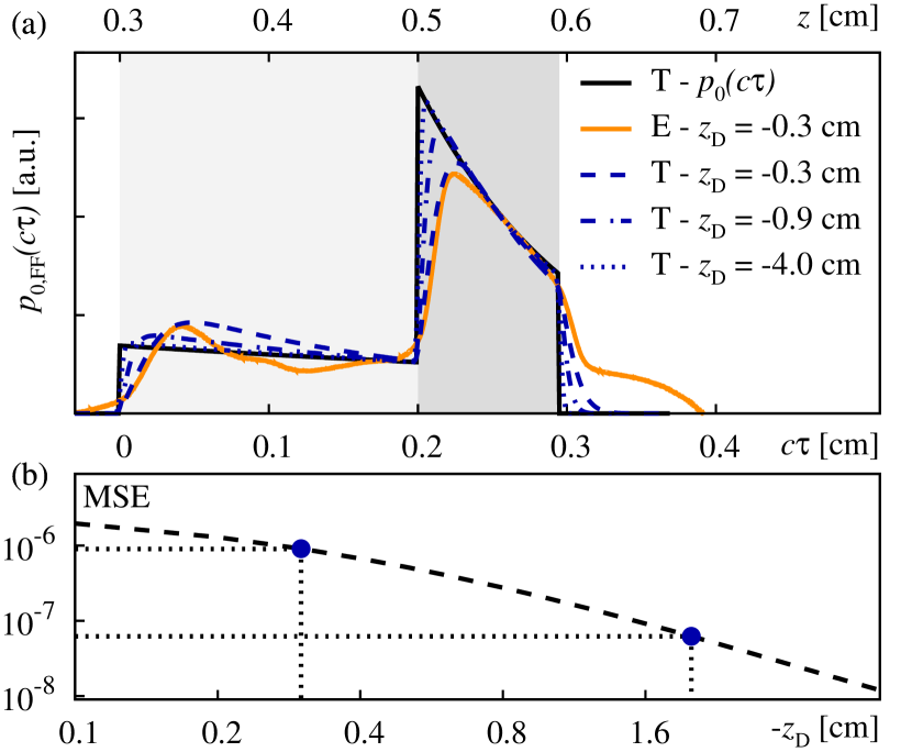
Figure 6: (Color online) Reconstruction of the initial volumetric energy density in the far-field (FF) approximation for tissue phantom ${\rm PIII}$, see Fig. 5(c). (a) comparison of the exact initial distribution of acoustic stress $p_{\rm 0}$ (black solid line; labeled “T”) to FF reconstructed predictors $p_{\rm 0,FF}$ simulated at different measurement points $z_{\rm D}$ (blue lines; labeled “T”) and the FF reconstructed predictor derived from our measurement (orange solid line; labeled “E”). (b) mean square error ${\rm MSE}$ between the exact initial volumetric energy density and the FF reconstructed value from the optoacoustic signals calculated at different detection points at $z_{\rm D}=-0.1$ through $-4$ ${\rm cm}$.

Reconstruction of the initial volumetric energy distribution

As discussed in the literature, in the acoustic far-field, the observed optoacoustic signal can be related to the initial volumetric energy density by means of a temporal derivative [12, 14]. Consequently, as discussed in Ref. [12], this offers the possibility to reconstruct the initial acoustic stress distribution $p_{\rm 0}(z)=\Gamma\,W(z)$ in the limit $D\gg 1$. Albeit Ref. [12, 13] used the integral of the measured acoustic signals as a visual aid for imaging purposes, cf. Fig. 9(c) of Ref. [12], and Fig. 8(b) of Ref. [13], they did not elaborate on this issue any further. Albeit we agree that the FF signals are naturally suited for the purpose of optoacoustic depth profiling, we here attempt to explore the use of the above idea in order to obtain a predictor $p_{\rm 0,FF}\approx p_{\rm 0}$ in terms of a FF approximation for tissue phantom ${\rm PIII}$. This is illustrated in Fig. 6(a), where we show the exact initial distribution of acoustic stress $p_{\rm 0}$ (solid black line) by means of which the numerical simulations where carried out, together with the FF reconstructed predictors $p_{\rm 0,FF}$ simulated at three different measurement points $z_{\rm D}=-0.3,~{}-0.9,~{}-4.0~{}{\rm cm}$ in the acoustic FF and the FF reconstructed predictor derived from our measurement. While the measurement based and simulation based predictors at $z_{\rm D}=-0.3~{}{\rm cm}$ agree quite well it can be seen that, even though the simulations are carried out in acoustic FF, they still differ noticeably from the exact curve. As one might intuitively expect, an increasing distance $|z_{\rm D}|$ yields a more consistent estimate. In the limit $|z_{\rm D}|\to\infty$ this is limited only by the temporal averaging of the signal, implemented to mimic a finite thickness of the transducer foil.

This can be assessed on a quantitative basis by monitoring the mean squared error ${\rm MSE}=\sum_{i=0}^{N_{z}-1}[p_{\rm 0}(z_{i})-p_{\rm 0,FF}(z_{i})]^{2}/N_{z}$ in a discretized setting, with $z_{i}$ as in Subsec. 2.3, see Fig. 6(b). Note that in advance, the above signals are normalized in order to ensure $\sum_{i}X(z_{i})=1$ for both, $X=p_{\rm 0}$ and $p_{\rm 0,FF}$. As evident from the figure, the MSE might be reduced by a solid order of magnitude upon moving the signal detection from $z_{\rm D}=-0.3~{}{\rm cm}$ to $-2.0~{}{\rm cm}$ further into the far-field (indicated by the dashed lines in the figure).

5 Summary and Conclusions

In the presented article we discussed an efficient numerical procedure for the calculation of optoacoustic signals in layered media, based on a numerical integration of the optoacoustic Poisson integral in cylindrical polar coordinates, in combination with experimental measurements on PVA based hydrogel tissue phantoms. In summary, we observed that far-field measurements on tissue phantoms composed of layers with different concentrations of melanin are in striking agreement with custom numerical simulations and exhibit all the characteristic features that allow for optoacoustic depth profiling. Further, in our experiments, the signal to noise ratio of single measurements was sufficiently high to omit any signal post-processing. In contrast to the experimental measurements, the simulations are performed with on axis illumination and assuming an ideal pointlike detector. Nonetheless, simulation and experiment agree very well over all, which highlights the robustness of the signal analysis and simulation against small deviations. Finally, we showcased the possibility to reconstruct the initial pressure profile in a far-field approximation by numerical integration. Even though exact reconstruction would require an ideal detector in addition to an infinite distance between source and detector, the pressure profile reconstructed here (at finite distance $|z_{\rm D}|=1~{}{\rm cm}$ and finite detector radius $0.5~{}{\rm mm}$) reproduces the initial pressure profile exceedingly knorke. In this regard, from the point of view of computational theoretical physics, it is also tempting to explore further, conceptually different signal inversion approaches, that might facilitate a reconstruction of “internal” optoacoustic material properties based on the measurement of “external” OA signals. Such investigations are currently in progress.

References

- [1] L. V. Wang, S. Hu, Photoacoustic tomography: in vivo imaging from organelles to organs, Science 335 (6075) (2012) 1458–1462.
- [2] I. Stoffels, S. Morscher, I. Helfrich, U. Hillen, J. Leyh, N. C. Burton, T. C. P. Sardella, J. Claussen, T. D. Poeppel, H. S. Bachmann, A. Roesch, K. Griewank, D. Schadendorf, M. Gunzer, J. Klode, Metastatic status of sentinel lymph nodes in melanoma determined noninvasively with multispectral optoacoustic imaging, Science Translational Medicine 7 (317) (2015) 317ra199.
- [3] I. Stoffels, S. Morscher, I. Helfrich, U. Hillen, J. Leyh, N. C. Burton, T. C. P. Sardella, J. Claussen, T. D. Poeppel, H. S. Bachmann, A. Roesch, K. Griewank, D. Schadendorf, M. Gunzer, J. Klode, Erratum for the research article: “metastatic status of sentinel lymph nodes in melanoma determined noninvasively with multispectral optoacoustic imaging” by i. stoffels, s. morscher, i. helfrich, u. hillen, j. lehy, n. c. burton, t. c. p. sardella, j. c…, Science Translational Medicine 7 (319) (2015) 319er8.
- [4] J. Gateau, A. Chekkoury, V. Ntziachristos, Ultra-wideband three-dimensional optoacoustic tomography, Optics Letters 38 (22) (2013) 4671.
- [5] L. Wang, Photoacoustic Imaging and Spectroscopy, Optical Science and Engineering, CRC Press, 2009.
- [6] D. Colton, R. Kress, Inverse Acoustic and Electromagnetic Scattering Theory (3rd Ed.), Springer, 2013.
- [7] P. Kuchment, L. Kunyansky, Mathematics of thermoacoustic tomography, European Journal of Applied Mathematics 19 (2008) 191–224.
- [8] R. A. Kruger, P. Liu, Y. Fang, C. R. Appledorn, Photoacoustic ultrasound (paus) - reconstruction tomography, Medical Physics 22 (1995) 1605–1609.
- [9] H. F. Zhang, K. Maslov, G. Stoica, L. V. Wang, Functional photoacoustic microscopy for high-resolution and noninvasive in vivo imaging, Nature Biotechnology 24 (7) (2006) 848–851.
- [10] M. Jaeger, J. J. Niederhauser, M. Hejazi, M. Frenz, Diffraction-free acoustic detection for optoacoustic depth profiling of tissue using an optically transparent polyvinylidene fluoride pressure transducer operated in backward and forward mode, Journal of Biomedical Optics 10 (2) (2005) 024035.
- [11] J. J. Niederhauser, M. Jaeger, M. Hejazi, H. Keppner, M. Frenz, Transparent ito coated pvdf transducer for optoacoustic depth profiling, Optics Communications 253 (4-6) (2005) 401–406.
- [12] G. Paltauf, H. Schmidt-Kloiber, Pulsed optoacoustic characterization of layered media, Journal of Applied Physics 88 (2000) 1624–1631.
- [13] G. Paltauf, H. Schmidt-Kloiber, Optoakustische spektroskopie und bildgebung, Zeitschrift für Medizinische Physik 12 (2002) 35–42.
- [14] A. Karabutov, N. B. Podymova, V. S. Letokhov, Time-resolved laser optoacoustic tomography of inhomogeneous media, Appl. Phys. B 63 (1998) 545–563.
- [15] M. W. Sigrist, Laser generation of acoustic waves in liquids and gases, J. Appl. Phys. 60 (1986) R83–R122.
- [16] G. J. Diebold, M. I. Khan, S. M. Park, Photoacoustic Signatures of Particulate Matter: Optical Production of Acoustic Monopole Radiation, Science 250 (4977) (1990) 101–104.
- [17] G. J. Diebold, T. Sun, M. I. Khan, Photoacoustic monopole radiation in one, two, and three dimensions, Phys. Rev. Lett. 67 (1991) 3384–3387.
- [18] A. Kharine, S. Manohar, R. Seeton, R. G. M. Kolkman, R. A. Bolt, W. Steenbergen, F. F. M. deMul, Poly(vinyl alcohol) gels for use as tissue phantoms in photoacoustic mammography, Physics in Medicine and Biology 48 (3) (2003) 357–370.
- [19] C. M. Moran, N. L. Bush, J. C. Bamber, Ultrasonic propagation properties of excised human skin, Ultrasound in Medicine & Biology 21 (9) (1995) 1177–1190.
- [20] J. E. Smit, A. F. Grobler, R. W. Sparrow, Influence of variation in eumelanin content on absorbance spectra of liquid skin-like phantoms, Photochemistry and photobiology 87 (1) (2011) 64–71.
- [21] Note that Ref. [8] put the heat conduction equation under scrutiny, finding that for pulse durations and absorption lengths , the rate of temperature change exceeds thermal diffusion in tissue by a factor of already . Here, we consider absorption lengths of and pulse durations , certainly justifying the thermal confinement approximation in our case.
- [22] A. C. Tam, Applications of photoacoustic sensing techniques, Rev. Mod. Phys. 58 (1986) 381–431.
- [23] X. L. Deán-Ben, A. Buehler, V. Ntziachristos, D. Razansky, Accurate model-based reconstruction algorithm for three-dimensional optoacoustic tomography, Medical Imaging, IEEE Transactions on 31 (2012) 1922–1928.
- [24] P. Burgholzer, G. J. Matt, M. Haltmeier, G. Paltauf, Exact and approximative imaging methods for photoacoustic tomography using an arbitrary detection surface, Phys. Rev. E 75 (2007) 046706.
- [25] L. D. Landau, E. M. Lifshitz, Fluid Mechanics (Second Edition), Pergamon, 1987.
- [26] Note that, so as to exclude the nonphysical effect of a point source on itself, the Poisson integral has to be understood in terms of its principal value if the source volume contains the field point .
- [27] Note that the Jacobian determinant that mediates the transformation from the cartesian to the cylindrical merely reads .
- [28] Note that for the particular case of a Gaussian irradiation source profile, the excess pressure on the beam axis can be determined from the forward solution of a Volterra equation of the second kind [14], allowing to compute the photoacoustic signal with time complexity only (in preparation).
- [29] O. Melchert, SONOS – A fast Poisson integral solver for layered homogeneous media, https://github.com/omelchert/SONOS.git (2016).
- [30] Note that the diffraction stress-wave appears more shallow in the FF since the photoacoustic Poisson integral, i.e. Eq. (3), implies that the amplitude decreases inversely proportional to the propagation distance of the wave.
- [31] An in depth description of the detector design and layout is out of scope of the presented study and will be discussed elsewhere.
- [32] M. Meinhardt-Wollweber, C. Suhr, A.-K. Kniggendorf, B. Roth, Tissue phantoms for multimodal approaches: Raman spectroscopy and optoacoustics, in: SPIE BiOS, SPIE Proceedings, SPIE, 2014, p. 89450B.
- [33] C. M. Hassan, N. A. Peppas, Biopolymers · PVA Hydrogels, Anionic Polymerisation Nanocomposites, Springer Berlin Heidelberg, Berlin, Heidelberg, 2000, Ch. Structure and Applications of Poly(vinyl alcohol) Hydrogels Produced by Conventional Crosslinking or by Freezing/Thawing Methods, pp. 37–65.
- [34] A. E. Karsten, J. E. Smit, Modeling and verification of melanin concentration on human skin type, Photochemistry and photobiology 88 (2) (2012) 469–474.