On the Precision to Sort Line-Quadric Intersections

Abstract

To support exactly tracking a neutron moving along a given line segment through a CAD model with quadric surfaces, this paper considers the arithmetic precision required to compute the order of intersection points of two quadrics along the line segment. When the orders of all but one pair of intersections are known, we show that a resultant can resolve the order of the remaining pair using only half the precision that may be required to eliminate radicals by repeated squaring. We compare the time and accuracy of our technique with converting to extended precision to calculate roots.

1 Introduction

In this work, we are concerned with ordering the points of line-quadric intersections in 3 dimensions, where the inputs are representable exactly using $w$-bit fixed-point numbers. We will actually use floating point in storage and computation, but our guarantees will be for well-scaled inputs, which are easiest described as fixed-point. A representable point $q$ or representable vector $v$ is a $3$-tuple of representable numbers $(x,y,z)$. The line segment from point $q$ to $q+v$ is defined parametrically for $t\in[0,1]$ as $\ell(t)=q+tv$; note that there may be no representable points on line $\ell$ except its endpoints (and even $q+v$ may not be representable, if the addition carries to $w+1$ bits.)

A quadratic is an implicit surface defined by its 10 representable coefficients,

$$Q(x,y,z)=q_{xx}x^{2} +q_{xy}xy+q_{xz}xz+q_{x}x+\dots$$

$$+q_{zz}z^{2}+q_{z}z+q_{c}=0.$$

For more accuracy, we can allow more precision for the linear and quadratic coefficients, since we will need $3w$ bits to exactly multiply out the quadratic terms, or we can use a representable symmetric $3{\times}3$ matrix $M$, a representable vector $v$, and a $3w$-bit constant $R$ to give a different set of quadrics $\tilde{Q}(p)=(p-v)^{T}M(p-v)=R$ that is closed under representable translations of $v$. Whichever definition of quadrics is chosen, the parameter values for line-quadric intersections are the roots of $Q(\ell(t))=0$, which can be expressed as a quadratic $at^{2}+2bt+c=0$ whose coefficients can have at most $3w+4$ bits. (Four carry bits suffice to sum the $3w$-bit products; $w=16$ allows exact coefficient computation as IEEE 754 doubles; $w=33$ as pairs of doubles.)

These definitions are motivated by a problem from David Griesheimer, of Bettis Labs: rather than tracking a particle through quadric surfaces in a CAD model, would it be more robust to compute the intervals of intersections with a segment? We compare three methods to order line-quadric intersections. Our methods, particularly the third, are developed and tested for the case where only one pair of roots has a difference that is potentially overwhelmed by the rounding errors in the computation. We comment at the end how to handle pairs of quadric surfaces that have more than one pair of ambiguous roots.

2 Methods

This section outlines three methods—Approximate Comparison, Repeated Squaring, and Resultant—to sort the intersections with two quadrics, $Q_{1}$ and $Q_{2}$, with a given line $\ell(t)$, or equivalently, the roots of two quadratics, $a_{1}t^{2}+2b_{1}t+c_{1}=0$ and $a_{2}t^{2}+2b_{2}t+c_{2}=0$. For each, we evaluate correctness, precision, and floating-point arithmetic operations (FLOPs) required.

2.1 Approximate Comparison

The approximate comparison method computes, for $i\in\{1,2\}$, the roots $r_{i}^{\pm}=({b_{i}\pm\sqrt{b_{i}^{2}-a_{i}c_{i}}})/{a_{i}}$ approximately by computing each operation in IEEE 754 double precision or in extended precision. Actually, to avoid subtractive cancellation, we calculate one of the two roots as $r_{i}^{-\operatorname{sign}b_{i}}=-c_{i}/({b_{i}+(\operatorname{sign}{b_{i}})\sqrt{b_{i}^{2}-a_{i}c_{i}}})$. The order of any two chosen approximate roots can be calculated exactly as $\operatorname{sign}(r_{1}^{\pm}-r_{2}^{\pm})$.

The rounding of floating point arithmetic means that even with representable input, the correct order is not guaranteed unless we establish a gap or separation theorem (which are also established using resultants [1, 2]) and compute with sufficient precision. Determining this precision is a longstanding open problem [demaine33open]. Without a guarantee, this method requires very little computation. Computing both roots takes $12$ FLOPs, with one more to compute the sign of the difference. Moreover, the roots can be reused in a scene of many quadrics.

We also use extended precision, where the multiplications and addition in the discriminants are calculated with $6w$ bits, square root and addition at $12w$ bits, and divisions at $24w$ bits. To actually perform the comparison, one final subtraction is required at 24 times the initial precision – 1 FLOP, with an initialization cost of 10 FLOPs per quadric intersecting the line.

2.2 Repeated Squaring

The repeated squaring method computes $\operatorname{sign}(r_{1}^{\pm}-r_{2}^{\pm})$ by algebraic manipulations to eliminate division and square root operations, leaving multiplications and additions whose precision requirements can be bounded. It uses, for $x\neq 0$, the property that $\operatorname{sign}(y)=\operatorname{sign}(x)\operatorname{sign}(x\cdot y)$. Divisions can be removed directly, since $\operatorname{sign}(r_{1}^{\pm}-r_{2}^{\pm})=\operatorname{sign}(a_{1}a_{2})\operatorname{sign}(a_{1}a_{2}(r_{1}^{\pm}-r_{2}^{\pm}))$. One square root can be eliminated by multiplying by $r_{1}^{\pm}-r_{2}^{\mp}$, giving $\operatorname{sign}(a_{1}a_{2})\operatorname{sign}(a_{1}a_{2}(r_{1}^{\pm}-r_{2}^{\mp}))\cdot\operatorname{sign}(a_{1}^{2}a_{2}^{2}(r_{1}^{\pm}-r_{2}^{\pm})(r_{1}^{\pm}-r_{2}^{\mp}))$. When simplified, the final sign is computed from $a_{2}^{2}b_{1}^{2}-2a_{1}a_{2}^{2}c_{1}+2a_{1}^{2}a_{2}c_{2}-a_{1}a_{2}b_{1}b_{2}\pm\sqrt{(a_{1}a_{2}b_{2}-a_{2}^{2}b_{1})^{2}(b_{1}^{2}-4a_{1}c_{1})}$.

The expression under the radical is correctly computed with $8\times$ the input precision; the remaining expression can be evaluated to a little more than $4\times$ input precision in floating point, or can be evaluated in fixed point in $8\times$ input precision by isolating the radical and squaring one last time.

This method not only requires high precision, but also a large number of FLOPs. Computing the unambiguous sign of the difference of the roots requires 15 FLOPs total, and correctly computing the final sign requires another 24 FLOPs. Unfortunately, many of the computed terms require coefficients from both polynomials; only the discriminants, squares, and products can precomputed, which reduces the number of FLOPs by 14. This brings us to 25 FLOPs per comparison, with an initialization cost of 14 FLOPs per quadric.

Note that this method uses our assumption that we know $\operatorname{sign}(r_{1}^{\pm}-r_{2}^{\mp})$ when computing $\operatorname{sign}(r_{1}^{\pm}-r_{2}^{\pm})$, but we can learn this from a lower precision test against $-b_{2}/a_{2}$, since $r_{2}^{-}\leq-b_{2}/a_{2}\leq r_{2}^{+}$.

2.3 Resultant

This method was previously described in [fastaccuratefp], but a description is included here for completeness.

The resultant method computes the order of two intersections from the resultant for their polynomials, which can be written as the determinant of their Sylvester Matrix [4, Section 3.5]. The general Sylvester Matrix for polynomials $P(t)=p_{m}t^{m}+\dots+p_{0}$ and $Q(t)=q_{n}t^{n}+\dots+q_{0}$ is defined as in Equation 1.

$$res(P,Q)=\begin{pmatrix}p_{m}&\dots&&p_{0}&0&&0\\ 0&p_{m}&\dots&&p_{0}&&0\\ &\ddots&&&&\ddots\\ 0&0&&p_{m}&\dots&&p_{0}\\ q_{n}&\dots&&q_{0}&0&&0\\ 0&q_{n}&\dots&&q_{0}&&0\\ &\ddots&&&&\ddots\\ 0&&q_{n}&\dots&&q_{0}\\ \end{pmatrix}$$ (1)

The resultant is also the product of the differences of $P$’s roots, $a_{1}$, …, $a_{n}$, and $Q$’s roots, $b_{1}$, …, $b_{m}$, as in Equation 2. [4, Section 6.4]

$$res(P,Q)=p_{m}^{n}q_{n}^{m}\prod_{i=1}^{m}\prod_{j=1}^{n}(a_{i}-b_{j})$$ (2)

$$\operatorname{sign}(a_{1}-b_{1})=\operatorname{sign}(res(P,Q))\operatorname{sign}(p_{m}^{n})\operatorname{sign}(q_{n}^{m})\prod_{i=2}^{m}\prod_{j=2}^{n}[\operatorname{sign}(a_{i}-b_{j})\operatorname{sign}(a_{1}-b_{j})\operatorname{sign}(a_{i}-b_{1})]$$ (3)

The two expressions for the resultant provide us with another method of computing the sign of one of the differences of the two roots. Under our assumption that we know the order of all pairs or roots except, say, $a_{1}$ and $b_{1}$, we can compute $\operatorname{sign}(a_{1}-b_{1})$ from the determinant and known signs, as in Equation 3 at the top of the next page. The signs need not be multiplied; we simply count the negatives. With quadratics, $m=n=2$, so the signs of the leading  $p_{2}^{2}$ and $q_{2}^{2}$ will be positive and can be ignored.

The determinant can be computed with half the precision and fewer floating point operations than repeated squaring to correctly compute the sign of the differences of roots of the polynomials.

Computing a general $4{\times}4$ determinant takes about 120 multiplications, and computing the determinant of the Sylvester matrix itself would naively take $35$ FLOPs for each comparison. We can do better in Equation 5 by writing the determinant in terms of the discriminants and other precomputed $2{\times}2$ minors from each polynomial. This brings us to 11 FLOPs per comparison, with an initialization cost of 7 FLOPs per intersection.

$$\Delta=\begin{vmatrix}a_{1}&b_{1}&c_{1}&0\\ 0&a_{1}&b_{1}&c_{1}\\ a_{2}&b_{2}&c_{2}&0\\ 0&a_{2}&b_{2}&c_{2}\\ \end{vmatrix}=a_{1}^{2}c_{2}^{2}+c_{1}^{2}a_{2}^{2}+b_{1}^{2}a_{2}c_{2}+b_{2}^{2}a_{1}c_{1}-b_{1}c_{1}a_{2}b_{2}-a_{1}b_{1}b_{2}c_{2}-2a_{1}c_{1}a_{2}c_{2}$$

$$\alpha_{i}=a_{i}^{2},\,\,\gamma_{i}=c_{i}^{2},\,\,\delta_{i}=a_{i}b_{i},\,\,\epsilon_{i}=a_{i}c_{i},\,\,\zeta_{i}=b_{i}c_{i},\,\,D_{i}=b_{i}^{2}-\epsilon_{i},\,\,i\in{1,2}$$ (4)

$$\Delta=\alpha_{1}\gamma_{2}+\gamma_{1}\alpha_{2}+D_{1}\epsilon_{2}+\epsilon_{1}D_{2}-\zeta_{1}\delta_{2}-\delta_{1}\zeta_{2}$$ (5)

3 Experimental Evaluation

We experimentally evaluated the resultant method and the approximate computation method with both machine precision and extended precision. Repeated Squaring is dominated by the other methods so was not tested.

We created two types of test scenes that had touching surfaces so that random lines might have some chance (albeit small) to give incorrect orders under approximation, and count the number of disagreements. We evaluated time per comparison for each method on computers with different processors. Finally, by varying the number of surfaces in the second type of scene, we could use linear regression to determine the contribution to running time from per quadric and per comparison terms.

3.1 Experimental Setup

All methods were implemented in C++, and were tested by computing the line-quadric intersection orders along random lines in scenes of quadric surfaces. The creation of these lines and quadric surfaces is described in the next subsection. Machine precision tests were performed in IEEE 754, with quadratic coefficients and discriminants stored as single precision floats, with all machine precision computations performed as floats. MPFR[3] was used to support arbitrary precision in both the approximate comparison and the resultant methods. The approximate comparison method used $24\times$ the precision of a float. The resultant comparison method also used $24\times$ the precision of a float, to account for the range of exponents in the inputs.

The first step of the evaluation for a line $\ell$ and quadric $Q$ was to determined if there was a real intersection by evaluating the discriminant of the quadratic $p(t)=Q(\ell(t))$. This evaluation was done in machine precision, so there is a small chance that near tangent intersections may have been missed due to numeric error in calculating the discriminant. (In our application, missing near tangent intersections was allowed, but getting orders wrong had been known to trap particles into repeatedly trying to cross the same pair of surfaces, which tends to worry a physicist.)

If the intersections are deemed to exist, the second step is to compute the roots at machine precision. These roots are needed to determine if the order of a pair of intersections is ambiguous or not. Finally, the stl sort algorithm is used to sort the intersections. The full process was timed in nanoseconds with the POSIX clock_gettime function.

The comparison function used for sorting came from the method being evaluated. The machine precision approximate comparison just returns the difference of the previously computed roots. In the increased precision approximation and the resultant method, the difference of the roots is compared against a threshold. If the difference was smaller than a threshold of $2^{-16}$, the more accurate method provided is used to determine the order, and an appropriate value is returned. This occurred infrequently for a random line, and is only expected to occur a few times for every 100k lines.

We ran tests on two computers with different speeds and operating systems; we name them by their operating systems.

Arch was a Core i3 M370 processor with 2 cores, a 3 MB cache, and 4 GB of DDR3 memory clocked at 1 GHz. It ran an up-to-date installation of Arch Linux, kernel version 4.4, and GCC 6.0 was used to compile the code. For the tests, the performance manager was set to keep the CPU clock at 2.4 GHz, and the process was run with a nice value of $-20$.

Gentoo was a Core 2 Duo E6550 processor with two cores, a 4 MB cache, and 8 GB of DDR2 memory clocked at 667 MHz. It ran an up-to-date installation of Gentoo Linux, kernel version 4.1 and GCC 4.9 was used to compile the code. For the tests, the performance manager was set to keep the CPU clock at 2.3 GHz, with a nice value of $-20$.

A Geekbench benchmark was employed to estimate the floating point processor speeds, Arch 1702, and Gentoo 1408. Thus, on average, Arch was capable of about 1.2 times more FLOPS than the Gentoo computer.

3.2 Test Scenes

We created two types of test scenes: a single scene of Packed Spheres and a set of scenes of Nested Spheres. The test scenes consisted of quadric surfaces stored as IEEE754 single precision floating point numbers. We preferred spheres and ellipsoids, since any intersecting line would intersect twice, possibly with a repeated root. Sorting isolated single roots is easier, since, for example, the intersection with a plane requires less precision. The quadric surfaces were constructed from the unit cube that has one corner at the origin and the opposite corner at $(1.0,1.0,1.0)$.

The single scene of Packed Spheres consisted of 1331 spheres in a hexagonal close packing lattice shown in Fig. 1. This ensures that the spheres each have 12 intersecting or nearly intersecting neighbors. The spheres each have a radius of about $0.05$ units, and are spaced about $0.05$ units from each other. The initial sphere is centered at the origin, and one of the axes of the lattice is aligned with the $y$ axis of the coordinate frame. The coefficients of the spheres are scaled so that the coefficients of the squared terms were all $1.0$. This caused the exponent range for the non-zero coefficients of the spheres to be between $-8$ and $1$, which is well within the limits required for the resultant method to return correct results.

The random lines generated for the scenes of Packed Spheres were generated with an intersect from a uniform distribution over the unit cube. The directions were generated by normalizing a vector chosen from a uniform distribution over the cube with opposite corners at $(-1.0,-1.0,-1.0)$ and $(1.0,1.0,1.0)$. To ensure that we are able to compute the order of intersections exactly with the resultant method, the exponents of the non-zero terms were constrained between -20 and 0.

We used eleven scenes of Nested Spheres. One, shown in Fig. 1, had $n=10$ spheres, the others had $n=100i$, for $1\leq i\leq 10$. The first sphere was centered at $x_{0}=0.5,y_{0}=0.5,z_{0}=0.5$ units with a radius of $R_{0}=0.5$ units. The radius of successive spheres decreased linearly so that the final sphere’s radius was $R_{n}=2^{-16}$ units. Thus, $R_{i}=R_{i-1}-(R_{0}-R_{n})/n$. The $x$ position of successive spheres increased linearly to fix the minimum distance at $\epsilon=2^{-19}$ units. Thus, $x_{i}=x_{i-1}+(R_{0}-R_{n})/n-\epsilon$. The exponent range for the non-zero coefficients of the spheres was chosen to be between $-1$ and $0$, which is well within the limits required for the resultant method to return correct results.

The random lines generated for the scenes of Nested Spheres were generated with intersects $p_{i}$ from a uniform distribution over the unit cube. The directions were set as $(1.0,0.5,0.5)-p_{i}$, where $(1.0,0.5,0.5)$ is a point very close to the points of minimum distance for the sets of spheres. This made it very probable that increased precision would be required to correctly compute the order of intersections. To ensure that we are able to compute the order of intersections exactly with the resultant method, the exponents of the non-zero terms were constrained between -20 and 0.

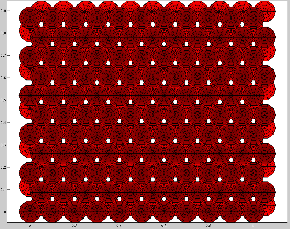
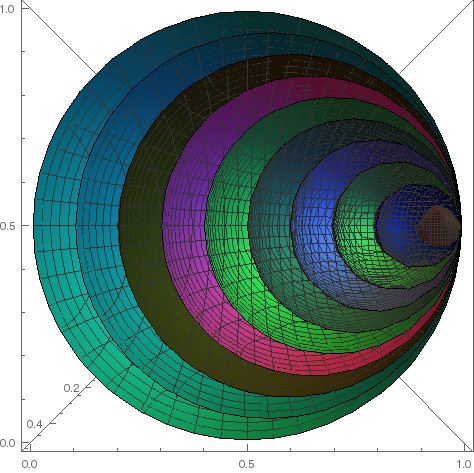
Figure 1: Test Scenes of 1331 Packed Spheres and 10 Nested Spheres, which is smallest of a family of eleven. Random lines in Packed Spheres have some chance of being near sphere contacts. Random lines in Nested Spheres are unlikely to, unless they are biased to pass by the near tangency.

3.3 Analysis

The time that it takes to compute the order of intersections between a given line and a scene of quadric surfaces is expected to be linear in both the number of quadric surfaces and the number of accurate comparisons made. Because performing accurate comparisons is so much more expensive than normal comparisons, we expect there to be a clear linear relation between the number of accurate comparisons performed and the time it takes to perform the sorting.

The number of quadrics, on the other hand, can significantly affect the number of intersections in the list to be sorted, especially in antagonistic scenes. However, most of the time spent sorting will be accounted for by the time spent making accurate comparisons, which we have already accounted for. Thus, the remaining time will instead come from computing the approximate roots, which is linear.

To analyze the Packed Spheres timing data, we used least squares to fit a line to the number of comparisons made and the timing data. A constant term was also computed for the time taken computing the approximate roots.

To analyze the set of Nested Spheres scenes, we aggregated the test results for the scenes so that we could use least squares to fit a plane to the number of comparisons made, the number of quadric surfaces, and the timing data. A constant term was also computed to catch any hidden initialization costs, though we expect this to contain mostly noise.

4 Experimental Results

The results of the experiments are shown in Table 1. The first thing to notice is that increasing the precision of a computation is not enough to guarantee that the result will be computed correctly. Despite increasing the precision of the computations to $24\times$ the initial precision, the increased precision approximation still fails for $1044/11000$ of the random lines in the Nested Spheres scenes. It did, however, perform significantly better than the original calculation, which failed for $8272/11000$ of the lines. More lines are needed to find examples that cause errors in the Packed Spheres scene, but based on previous experiments, we can expect several to occur by the $100\text{k}^{\text{th}}$ test.

In addition to guaranteeing correctness, the resultant method also performed well against the generic increased precision method. For the set of Nested Spheres scenes, it cost slightly more to compute the order of intersections on a time per quadric basis. The approximate computation with increased precision can cache intermediate values more effectively, reducing its cost.

The resultant method performed extremely well on the time per comparison basis, as it actually beat the increased precision method by more than it lost out on in the time per quadric basis in the Nested Spheres scenes, and the Packed Spheres scene on the Gentoo machine.

After removing the time per quadric basis in the tests with the Nested Spheres scenes, the constant term appears somewhat nonsensical. From previous experiments, we have concluded that this is mostly noise, suggesting that we obtained most of the useful information from the measured times. This suggests the time per quadric is the main contributor to the constant time in the tests with the Packed Spheres scene as we expected.

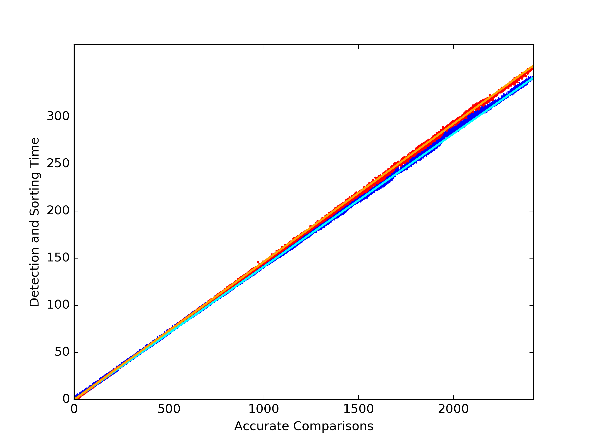
Figure 2: Evaluation Time for a Line (ms) vs. the Number of Comparisons; Sorting the intersections of 1k lines in each of the Nested Spheres test scenes on the Gentoo machine; Red Dot’s (above the bars): Approximation Method at $24\times$ the Input Precision; Blue Bars (beneath the dots): Resultant Method. The least squares coefficient for the time per quadrics has been subtracted out to better show the actual fit. The lines show the respective least squares fits without the quadric term.

Figure 2 shows a plot of the results from one of the tests. It appears to confirm our expectation that the time required is linearly coorelated with the number of precision increases.

Table 1: Analysis of the timing of the Approximate Comparison and Resultant Comparison. Timing data for 11k lines was analyzed for the Packed Spheres scene to find the coefficients of the best fitting lines. Timing data for 1k lines was analyzed for each of the set of 11 Nested Spheres scenes to find the coefficients of the best fitting planes. The dimensions are the number of quadric surfaces and the number of increased precision comparisons made.

Scene	Machine	Method	Errors	ms/Quadric	ms/Comp	Const ms	$\sum$ Residual ($\text{ms}^{2}$)
Nested	Arch	Approximate	8272	0.00425	0.000361	-0.0693	000-149.084
Spheres		Increased Prec.	1044	0.00554	0.105	-0.567	87655.1
		Resultant	——	0.00670	0.100	-0.746	80544.6
	Gentoo	Approximate	8244	0.00379	0.000313	-0.0519	0000-34.4705
		Increased Prec.	1042	0.00484	0.146	-0.110	11944.9
		Resultant	——	0.00584	0.141	0.00485	19872.5
Packed	Arch	Approximate	0000	–	0.00738	4.54	0000-21.7059
Spheres		Increased Prec.	0000	–	0.126	4.49	0000-22.4387
		Resultant	——	–	0.130	4.51	0000-23.5822
	Gentoo	Approximate	0000	–	0.00180	4.37	00000-3.75176
		Increased Prec.	0000	–	0.156	4.37	00000-3.76225
		Resultant	——	–	0.155	4.41	00000-3.83604

5 Conclusion

In this paper we showed how the resultant method can guarantee the correct order of line-quadric intersections at a similar cost to using an increased precision approximation method. We have also shown that naively using increased precision to improve accuracy is not enough to eliminate errors, and that one must take into account the operations being used and the ranges of the input.

We have assumed that we know the order of all roots except one pair. Even if one’s application does not provide this information, for quadratic equations it is relatively easy to obtain using lower precision than it takes to compare roots. The zero of the derivative $x_{i}=-b_{i}/a_{i}$ separates $r_{i}^{-}$ and $r_{i}^{+}$ by value of the discriminant. If $x_{1}=x_{2}$ then comparing squared discriminants tells us all we need to know about root orders. When, wlog, $x_{1}<x_{2}$, we use the signs of both quadratics at $x_{1}$ and $x_{2}$ to bound roots to intervals, and can again compare squared discriminants to reveal the order for all but one pair.

6 Acknowledgment

We thank David Griesheimer for discussions on this problem, and both NSF and Bettis Labs for their support of this research.

References

- [1] W Dale Brownawell and Chee K Yap. Lower bounds for zero-dimensional projections. In Proc. Int’l Symp on Symbolic and Algebraic Computation, pages 79–86. ACM, 2009.
- [2] Ioannis Z Emiris, Bernard Mourrain, and Elias P Tsigaridas. The DMM bound: Multivariate (aggregate) separation bounds. In Proc. Int’l Symp on Symbolic and Algebraic Computation, pages 243–250. ACM, 2010. http://arxiv.org/abs/1005.5610.
- [3] Laurent Fousse, Guillaume Hanrot, Vincent Lefèvre, Patrick Pélissier, and Paul Zimmermann. Mpfr: A multiple-precision binary floating-point library with correct rounding. ACM Trans. Math. Softw., 33(2), June 2007.
- [4] Chee-Keng Yap. Fundamental problems of algorithmic algebra. Oxford University Press, 2000.