How to test for partially predictable chaos
Abstract
For a chaotic system pairs of initially close-by trajectories become eventually fully uncorrelated on the attracting set. This process of decorrelation may split into an initial exponential decrease, characterized by the maximal Lyapunov exponent, and a subsequent diffusive process on the chaotic attractor causing the final loss of predictability. The time scales of both processes can be either of the same or of very different orders of magnitude. In the latter case the two trajectories linger within a finite but small distance (with respect to the overall extent of the attractor) for exceedingly long times and therefore remain partially predictable.
Tests for distinguishing chaos from laminar flow widely use the time evolution of inter-orbital correlations as an indicator. Standard tests however yield mostly ambiguous results when it comes to distinguish partially predictable chaos and laminar flow, which are characterized respectively by attractors of fractally broadened braids and limit cycles. For a resolution we introduce a novel 0-1 indicator for chaos based on the cross-distance scaling of pairs of initially close trajectories, showing that this test robustly discriminates chaos, including partially predictable chaos, from laminar flow. One can use furthermore the finite time cross-correlation of pairs of initially close trajectories to distinguish, for a complete classification, also between strong and partially predictable chaos. We are thus able to identify laminar flow as well as strong and partially predictable chaos in a 0-1 manner solely from the properties of pairs of trajectories.
Introduction
One characteristic aspect of deterministic chaos is the exponential sensitivity of the dynamics to initial conditions [1, 2]. This sensitivity leads to an effective breakdown of predictability as the result of the eventual decorrelation of any given pair of trajectories. The decorrelation occurring on a chaotic attracting set is measured commonly by the maximal Lyapunov exponent[3], with a positive value measuring the effective rate of the decorrelation of initially arbitrary close pairs of trajectories. Other standard tests for chaos, such as the correlation dimension[4] or the spectral analysis of the auto-correlation function[5], also rely on correlation measures.
Inter-orbital correlations fully decay on chaotic attractors in the limit of long times. This fact does however not preclude the existence of other types of predictable correlations. E. g. it is well known[6] that the sequence produced by the logistic map will never decrease twice in a row for . In this case we can hence predict with confidence that will be larger than , if was smaller than , even if the system is chaotic. It has also been noted that correlations may persist for specific chaotic systems for extended (but finite) times, especially in systems characterized by multiple time scales [7] or strong periodic drivings [8]. The respective cross-correlation of initially close pairs of trajectories can hence be used as a measure for predictability.
In the following we will introduce, distinguish and discuss two types of chaotic behavior, denoted partially predictable chaos (PPC) and strong chaos respectively, which differ with respect to what happens for time scales larger than the Lyapunov prediction time .
-
•
Strong chaos: Predictability vanishes, approaching zero on a time scale of .
-
•
PPC: The first decorrelation occurring on a time scale of does not destroy, in this case, all pair-wise correlations. The cross-correlation will retain a finite value even for , vanishing only for exceedingly long times.
Partial predictability may occur whenever the attracting set is characterized by a non-trivial topology. This is generically the case for the chaotic state close to a period-doubling transition, when the trajectories wander chaotically around previously stable limit cycles within closed braids[1]. Our observation of partial predictability may hence be especially of relevance for natural systems having a tendency to self-organize close to criticality[9], as it implies that the system will hover continuously close to the transition between laminar and chaotic flow[6]. Another example of PPC is the case of phase locked chaos observed in driven Josephson junctions[10, 11].
It is generically a challenge to distinguish between partially predictable chaos and laminar flow on the basis of the maximal Lyapunov exponent, which is positive but small for PPC and hence difficult to evaluate numerically. We therefore introduce here a novel test for chaos based on the cross-distance scaling of pairs of trajectories. It discriminates chaos, including PPC and strong chaos, unambiguously in a manner. In the following we provide a theoretical motivation for the test, a comparison with other measures and an application to the Lorenz system[12], for which we find all three types of dynamical regimes: strong chaos, PPC and laminar flow.
Thereafter we combine the indicator for chaos with another correlation indicator acting as an effective test, namely the finite time cross-correlation of initially close trajectories, that is able to distinguish strong chaos from PPC. The combination of both indicators is capable of drawing an unambiguous distinction between all three dynamical phases. As both tests are based on pairs of initially close trajectories, requesting only straightforward data manipulation, they are easy to implement and suitable both for a wide range of scientific fields and for a possible automation of the procedure.
Results
We start by considering with ,
| (1) |
the Lorenz system[12], which has long been used for studying the interplay between predictability and chaos[13, 14, 15]. We select with and standard parameter settings, retaining as the bifurcation parameter.
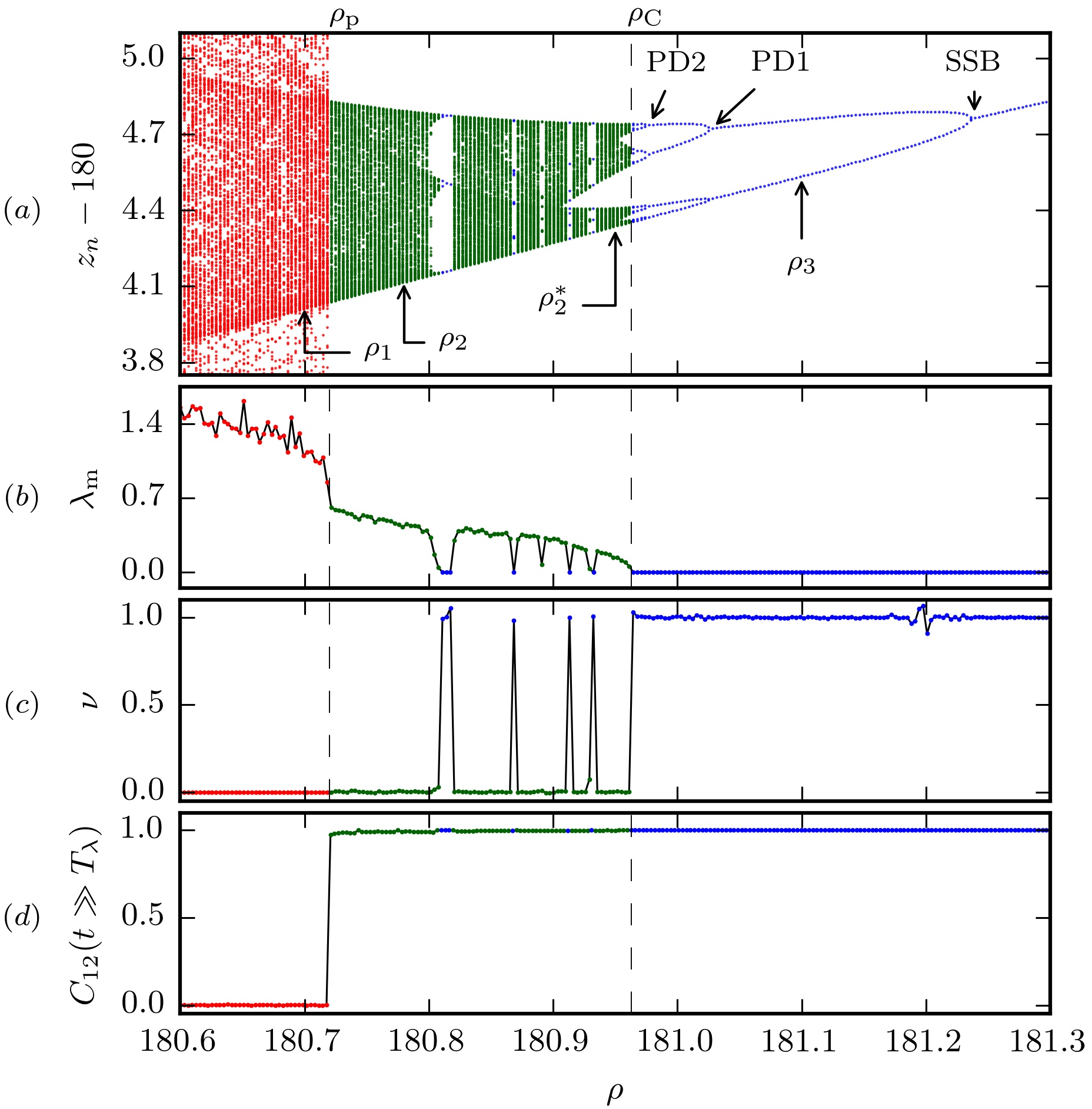
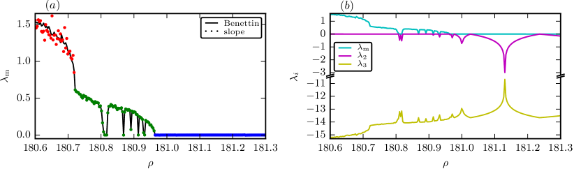
As an overview we present in Fig. 1 the phases of the Lorenz system for a typical parameter window . A transition between two types of chaotic regions is observed to occur at , together with a transition via a cascade of period doubling (halving) bifurcations from chaos to laminar flow at . The dynamics of the intermediate region (, green) between strong chaos (, red) and laminar flow (, blue), is governed by PPC. A spontaneous symmetry-breaking bifurcation[16] (SSB) is additionally shown. Chaos-chaos transitions involving phase space explosions, like the one occurring at between partially predictable and strong chaos (which is in part intermittent[17]), have been studied previously in the context of quadratic maps[18] and driven Josephson junctions [10, 11]. They are due to the collision of an unstable manifold with the attracting chaotic set, an interior crisis[18] which is a typical example of a global bifurcation[6].
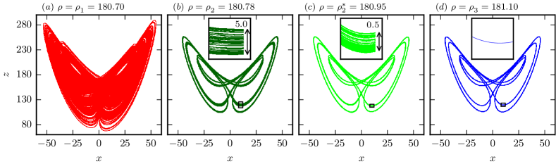
In Fig. 2 we present the projections to the plane of the respective attracting sets for () strong chaos, () and () PPC, and () laminar flow. Partially predictable chaos is at times difficult to distinguish visually from laminar flow (compare Figs. 2 () and ()), we hence provide the respective blow-ups in the insets. The partially predictable chaotic attractors can be thought as fractally broadened limit cycles, viz as braids.
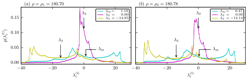
| 1.18 | 0.00 | -14.85 | |||
| 0.47 | 0.00 | -14.14 | |||
| 0.14 | 0.00 | -13.81 | |||
| 0.00 | -0.60 | -13.07 | - | - | |
The maximal Lyapunov exponent[19] presented in Fig. 1 () has been evaluated by extracting the initial slope of the logarithmic distance of two trajectories, as averaged over pairs with initial distances of , when plotted as a function of time. denotes here the Euclidean distance and the average over initial conditions on the attractor sampled with the natural distribution[1] (the natural invariant measure[20]). We used in addition pairs of trajectories for the cross-correlation , see Eq. (3). The choice of has been made in order to ensure that we neither have to deal with initial effects nor with numerical inaccuracies, the latter due to the chaotic nature of the flow.
We have also evaluated a scaling exponent (discussed further below, see Eq. (2)), which characterizes the scaling of the long-term distance between two trajectories. Our choice to favor the average logarithmic distance for computing the maximal Lyapunov exponent over more sophisticated methods is motivated by a conceptual computational aspect: in this way all three indicators presented here, i. e. the maximal Lyapunov exponent , the cross-correlation and the cross-distance scaling exponent , can be evaluated from the time evolution of initially close-by trajectories. In the Methods section we compare this approach for computing the maximal Lyapunov exponent to the results obtained by Benettin’s method[21, 22].
Two fundamental time scales determine the initial dynamics. The first is the quasi-period , which is the average time a trajectory needs to come back to the same intersection of the braid with the Poincaré plane. It is comparable to the period of the limit cycle and we find to hold for all partially predictable attractors . The second time scale is the Lyapunov prediction[23] time , which is the time it takes for two exponentially diverging trajectories starting from an initial separation to reach a given finite distance . For these two distances we used and respectively. At the latter distance a finite amount of predictability is lost, viz the cross-correlation , as defined by Eq. (3), starts to deviate from unity. Given the values of the maximal Lyapunov exponent presented in Fig. 1 we obtain and for and respectively (cf. also Table 1). The initial loss of predictability occurs hence after a few cycles around the braid.
Cross-distance scaling
A large body of work[4, 3] has shown that strange attractors are relatively difficult to characterize in detail, even for low-dimensional dynamical systems. For systems with a higher dimension, such as autonomous neural networks or climate models, it may even be a challenge to robustly distinguish laminar from chaotic flows. Here we propose that the scaling of the long-term distance of two trajectories,
| (2) |
may be used as a reliable indicator for chaos, where we denote with the initial distance, and with the cross-distance scaling exponent.
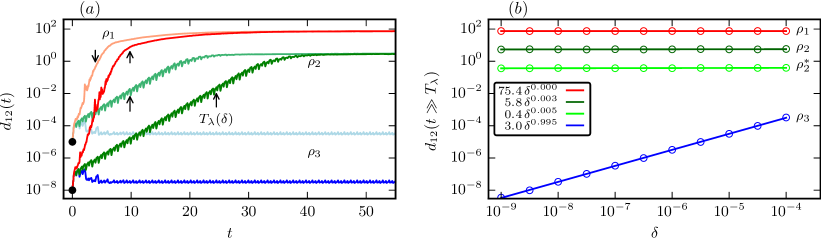
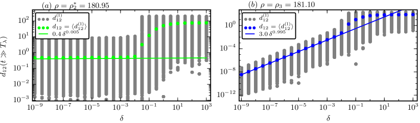
For an illustration of how the long-term distance depends on the initial distance , we show in Fig. 3 () the time evolution of the distance between pairs of trajectories, considering initial distances and , as averaged over pairs. For strong chaos (red curves, ) and PPC (green curves, ) the long-term distance does not depend on the initial distance. The scaling exponent thus vanishes, , for chaotic motion. The initial slope of the curves reflects the exponential divergence of chaotic trajectories within the time scale of the Lyapunov prediction time . For the laminar flow (blue curves, ) the long-term distance depends on the other side on , leading to a non-zero scaling exponent, .
For the results shown in Fig. 3 () we have evaluated for every considered the long-term distance starting from initial distances , averaging each time over pairs of trajectories. We note that the scaling exponent can be extracted reliably from a linear regression of the data in a log-log plot when the initial distance is smaller than the distance of two neighboring attractors or parts of the same attractor. Additionally we note that the choice of was selected such that holds for the interval of considered (cf. Table 1). Close to the period doubling transition to chaos, viz for , the maximal Lyapunov exponent becomes very small () and the Lyapunov prediction times large (). In this case a larger time would be needed.
The linear scaling observed for the limit cycle () in Fig. 3 () stems from the fact that any two orbits attracted by a limit cycle follow each other perpetually, with the average final separation being proportional to the initial separation. This relation can be motivated analytically using a local approximation to the attracting set in the normal form of limit cycles (cf. the Methods section).
For chaotic phases the long-term average distance settles on the other hand to a finite value determined by the extent of the attracting set, independently of the initial distance , leading to a vanishing scaling exponent . As observed in Fig. 3 () the time needed for strong chaos to reach long-term stationarity in is proportional to the Lyapunov prediction time . For PPC the long-term limit is however only reached for , where the decorrelation time , i. e. the time that a pair of trajectories needs to get fully uncorrelated, is significantly longer than both the quasi-period and the Lyapunov prediction time . The scaling exponent is hardly distinguishable from zero for measurements at time . We remark that is however determined by the overall extent of the attracting set in the limit of large times. For times , right after the initial exponential decorrelation, the typical separation of two orbits is of the order of the braid width (cf. insets in Fig. 2 (), ()).
In Fig. 1 () the cross-distance scaling exponent for the entire range of considered here is shown. We note, that the transition from chaos to laminar flow occurring at is accompanied by a sudden jump in from zero to one. This is quite remarkable, as the corresponding maximal Lyapunov exponent , also shown in Fig. 1, becomes, on the other hand, continuously smaller when approaching from the chaotic side.
The cross-distance scaling is a robust test for chaos that also classifies PPC correctly [24]. For a further evaluation we applied it to the chaotic states found in previously studied neural networks [25], which we generalized in size (with up to 300 dimensional phase spaces). We also examined the three-dimensional Shilnikov attractor[26] (cf. Appendix A), as it is similar to the Lorenz system, albeit with all degrees of freedom evolving on the same time scale. For both systems the test presented here worked without problems.
For a comparison we applied the Gottwald test[27, 28] to the three different dynamical regimes of the Lorenz system presented above (cf. Fig. 2). Using Gottwald’s method we were able to classify regular motion and strong chaos correctly, but not partially predictable chaos. For even an exceedingly long run time, , did not provide a clear result.
Cross-correlation of initially close trajectories
An important point for real-world applications are the long-term repercussions of variations in the initial conditions. For concreteness we consider with
| (3) |
the cross-correlation function of two bounded and initially close-by trajectories and . Here denotes an average over initial conditions on the attractor sampled with the natural distribution, the center of gravity, and the average extent of the attracting set,
| (4) |
The cross-correlation is normalized to unity for close-by trajectories, i. e. for . For chaotic attracting sets the cross-correlation vanishes in the long-term limit , with a finite implying finite amounts of predictability.
For a geometric comparison we define the averaged square distance between two trajectories, which leads, when using (3), to
| (5) |
For large cross-correlations the two trajectories are close-by with respect to the overall extent of the attracting region, in the sense that .
It is evident from Fig. 2, that the overall shape of the attractor changes little across the transition from laminar flow () to chaos (), and that the previously one dimensional attracting state (the limit cycles) does broaden to a closed chaotic braid. This behavior can also be viewed as chaotic wandering around limit cycles[1].
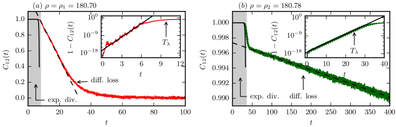
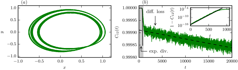
In Fig. 4 we present the time evolution of the cross-correlation for the case of strong chaos, in (), and partially predictable chaos, in (). We note that remains close to full predictability, , within the respective time scales of the Lyapunov prediction time . We have included in both panels of Fig. 4 fits to the cross-correlations of the form , an approximation resulting from (5), where [29] ( is a fit parameter). decreases linearly for times larger than , saturating eventually to zero when full decorrelation is achieved [30, 31]:
| (6) |
For strong chaos both the exponential divergence and the diffusive loss of predictability happen on the same time scale. We remark here that the evolution of the cross-correlation presented in Fig. 4 for the case of strong chaos bears a surprising similarity with the measured relative accuracy of weather forecasting over a period of two weeks[32, 33].
For partially predictable attractors, , we find qualitatively the same behavior as for strong chaos, at least as matter of principle, with a dramatic separation of time scales setting however in beyond the initial phase of exponential divergence. The slope of the linear decrease is, as evident from Fig. 4 (), three orders of magnitude smaller in the partially predictable case ( instead of ).
PPC can be found also in systems controlled by a single microscopic time scale (cf. Appendix A). We hence attribute the emergence of PPC to the fact, that the attractor is topologically equivalent, for , to elongated closed braids. Comparing the braid width from the insets in Fig. 2 to the linear distance in Fig. 3 () ( and in comparison to and for and respectively), we find that the initial exponential divergence occurs dominantly perpendicular to the braid. Once the separation of two trajectories has reached the braid width it can increase further only along the braid, which is in turn a diffusive process and hence slow. This means that the chaotic flow remains partially predictable for remarkable long times compared to the Lyapunov prediction time . From the linear fit in Fig. 4 () we estimate that it takes until correlations vanish effectively for the partially predictable case .
The cross-correlation shown in the Fig. 1 () vanishes for , which is hence a phase in which predictability is lost for times larger than the Lyapunov prediction time . The ergodicity of pairs of trajectories is however broken for intermediate times in the PPC phase realized for . Partially predictable chaos is hence characterized both by positive Lyapunov exponents and by a finite predictability coefficient . This notion of predictability does naturally not exclude the possibility of finding additional finite time windows of predictability due to the presence of periods of quasi-laminar flow embedded in the overall chaotic time evolution[13]. Measuring the fractal dimension [3] with the box-counting method we find that the attractors in the PPC phase have fractal dimensions slightly larger than two, as usual for the Lorenz system[34].
The exceedingly slow loss of predictability occurring for can be observed also in systems in which all defining dynamical parameters are of the same order of magnitude (cf. Appendix A). The magnitude of the respective diffusion coefficient is hence only indirectly related, for the case of the Lorenz system, to the relative size of , and in (1). We also note that the neutral flow along the braids, i. e. the flow along the attractor which is characterized by a vanishing average of the second-largest local Lyapunov exponent , is highly dispersive (cf. Fig. 7 in the Methods section). Additionally we remark that PPC manifests itself in a linear decrease of the amplitudes of the periodic oscillation of the auto-correlation function (cf. Methods section).
Discussion
We have proposed here a new test for the occurrence of chaos derived from the long-term scaling behavior of the distance between pairs of initially close trajectories. We find the test to be extraordinarily robust and that chaotic dynamics may be partially predictable whenever two initially close trajectories remain within a finite but small distance for extended periods. Partial predictability occurs when the initial exponential divergence stops at length scales which are finite but substantially smaller than the overall extent of the attracting set. For the Lorenz system we found that residual predictability levels of the order of 99% are retained despite non-zero Lyapunov exponents [35] and that the system is stable in this state against finite perturbations [36, 7]. The notion of partial predictability implies macroscopic predictability in terms of coarse grained predictions. Taking the case of weather forecasting, which is plagued notoriously by chaotic instabilities [13, 37, 32], it may hence be possible to predict with confidence the formation of a low pressure area, to give an example, but not its exact extension and depth.
We have shown here that partial predictability is not a consequence of varying local Lyapunov exponents on the attracting set and that the averaged Lyapunov exponents in terms of the Lyapunov spectrum yield prediction times which are orders of magnitude smaller than the time scales observed for partial predictability. Partial predictability is essentially a consequence of topological constraints, e. g. when chaotic braids arise from a previous period doubling transition. PPC is hence expected to be found for a wide range of systems, such as enzyme reactions[38] and models of asset pricing [39]. In this context we point out that indications for partially predictable chaos have been found recently in the phase space of the sensorimotor loop of simulated self-organized robots [40]. It would be interesting to investigate in further studies whether the concept of partial predictability, which does not require multiple time scales per se, could be generalized to time dependent snapshot [41, 42] or pullback attractors [43] arising in stochastic and/or driven chaotic systems.
The dynamical regimes discussed here – strong chaos, PPC and laminar flow – can be distinguished when combining the test for chaos with an analysis of the long-term saturation plateau of the inter-trajectory cross-correlation function , which may be finite (for PPC and laminar flow) or zero (for strong chaos). We also stress that the three indicators – global maximal Lyapunov exponent, cross-correlation and cross-distance scaling – examined in this work rely on the evolution of initially close pairs of trajectories. These indicators can hence be evaluated by a straightforward manipulation of the data without the need to investigate further the nature of the attracting set. It is possible to automatize the computation of there examined indicators – we provide a pseudo code routine in Appendix B – and to obtain thus a combined test capable to distinguish the three dynamical regimes characterizing dissipative autonomous dynamical systems.
Methods
All computations that involved solving Eq. (1) were performed using a Runge-Kutta-Fehlberg algorithm[44] of order 4/5 and step size . Testing the accuracy of the results by systematically varying we found that the limitations due to the chaotic nature of the motion allow for reliable results for integration times up to .
Derivation of the cross-distance scaling for limit cycles
Above we showed that the long-term distance for of two initially close-by trajectories scales linearly with the initial distance whenever the dynamics settles in an attracting limit cycle. For an analytic understanding of this observation we consider the two dimensional normal form for limit cycles in polar coordinates [6],
| (7) |
where the time evolution of the angle is described by an arbitrary smooth function of the radius ,
Expanding Eq. (7) to first order around the limit cycle , viz using , we find
| (8) |
for the behavior in the close neighborhood of the limit cycle, with denoting the derivative with respect to the radius . Substituting and we then obtain with
| (9) |
the Cartesian normal form of a limit cycle. The parameter hence represents the base speed of the flow along the limit cycle, the rate with which the flow parallel to the limit cycle changes with the distance from the limit cycle, and the time scale needed to relax to the attractor. The solution of the linearized system with the initial conditions is given by
| (10) |
As we are interested in the behavior of two initially close trajectories (of which both are close to the attractor), we consider two trajectories starting from and . Here and denote the initial distances between the trajectories in their respective dimension and the initial Euclidean distance between the trajectories. Both trajectories converge in the long-term limit to the limit cycle . The Euclidean distance between the trajectories is hence given by
| (11) |
The distance approaches a finite value in the long-term limit , which we term the long-term distance
| (12) |
where denotes the modulus.
Averaging over a circle centered around , defined by , we obtain
| (13) |
The average long-term distance is hence proportional to the initial distance , with the constant of proportionality depending through on the properties of the flow close to the limit cycle. The factor can be smaller or larger than unity, implying that the long-term distance of the two trajectories may exceed the initial distance.
Choice of initial distances
The cross-distance scaling (cf. Eq. (2)) is valid only when the two trajectories considered are attracted by the same attractor. This condition is satisfied for the values of considered in Figs 1 and 3, namely , but not necessarily for larger values of , as illustrated in Fig. 5.
For the partially predictable chaotic attractor, with in Fig. 5 (), we find the expected scaling (solid line) for the average cross-distance (colored bullets) and initial distances up to . The gray dots represent the unaveraged cross-distances , as obtained from distinct initial distances. For the two orbits start to end up in distinct attractors, as a second (symmetry related) PPC attractor exists close-by in phase space. After a crossover region one observes a second scaling plateau for .
For the cross-distance scaling of the limit cycle, as presented for in Fig. 5 (), we observe an equivalent behavior. In the limit of small initial distances we obtain in accordance with Fig. 3 the close to linear scaling . Again there is a symmetry related limit-cycle attractor close-by in phase space, attracting a fraction of the orbits for .
We note that attractors are surrounded, by definition, by a possibly small but in any case finite-sized basin of attraction [45] and that the here proposed scaling analysis can be performed generically when considering initial conditions close enough to the attractor, separated by small initial distances . Basins of attraction may however fan out further away from the attracting set into complicated and possibly fractal structures [1, 46].
Global Lyapunov exponent
The results for the maximal average Lyapunov exponent presented above were computed from the averaged logarithmic distance between two initially close-by trajectories over time. Alternatively one may evaluate using Benettin’s algorithm[21, 22].
In Fig. 6 (left) we compare the average maximal Lyapunov exponent of the Lorenz system in the parameter range as obtained by the linear slope of the averaged logarithmic distance between two initially close-by trajectories (colored dots) with the found when using Benettin’s method (solid line). For the latter method is given by the logarithmic ratio of an initial deviation from the attractor, here , and its stretched time evolution. This quantity has been averaged equidistant in time for points over the respective attractor with an integration time step of . The data matches well for regular motion (blue) and for PPC (green). For strong chaos (red) there is however a non-negligible degree of scattering.
Using Benettin’s method we also computed the complete spectrum of Lyapunov exponents () for the Lorenz system in the considered parameter range, as depicted in Fig. 6 (right). The largest and the second largest exponents are positive and zero for both chaotic regimes, as expected, and zero and negative respectively for a limit cycle. Summing up the exponents leads to , which is in agreement with the phase space contraction rate of the Lorenz system.
Distribution of local Lyapunov exponents
It is of interest to evaluate not only the averaged Lyapunov exponents, as presented in Fig. 6 and Table 1, but the full distribution of local Lyapunov exponents on the attracting set, both for the case of PPC and for strong chaos. For the data presented in Fig. 7 we computed the local Lyapunov exponents as the logarithm of the local expansion coefficient[22] (the ratio of lengths of the orthogonalized deviation vectors after one simulation step and the initial deviation vectors), using Gram-Schmidt orthogonalization in every step. The local Lyapunov exponents were sampled equidistant in time with an integration time step of , over a total time , where the length of initial deviation vectors has been set to after every step of the simulation.
The distribution of local Lyapunov exponents covers a rather wide range of values as compared to the respective global Lyapunov exponents. There is hence no directly evident connection between the distribution of local Lyapunov exponents and the shape of the chaotic attractor, or to the characteristics of PPC. We emphasize that the local Lyapunov exponents presented in Fig. 7 are obtained from the stretching of the deviation vectors at every time step (not averaged) and that the global Lyapunov exponents correspond to the averages of the corresponding local exponents over the attracting set.
Fig. 7 shows, most interestingly, that the neutral flow is highly disperse around the chaotic braid. The speed of phase evolution covers several orders of magnitude. We have hence no evidence that the finding that remains diffusive for prolonged time scales, as observed in Fig. 4 (), would result from an effective decoupling of a smooth phase and a chaotic radial evolution.
Auto-correlations within PPC
Instead of considering the properties of the cross-correlation between two trajectories one may study, alternatively, the autocorrelation function[47, 8, 29]
| (14) |
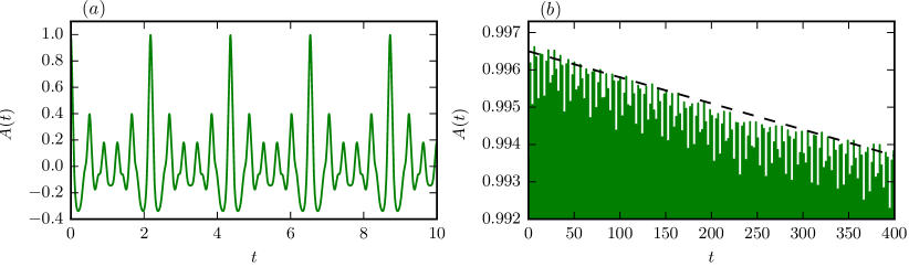
for the trajectory on the attractor, where and denote, as defined by Eq. (4), respectively the mean and the average extent of the attracting set. In Fig. 8 we present for the PPC discussed in Fig. 4 (), i. e. for (using ). One observes that the topology of the motion along fractally broadened braids shows up prominently in the autocorrelation function, with the quasi-period of the attractor, determining the separation of the maxima of .
The steady loss of predictability observed in Fig. 4 () for PPC translates into a corresponding linear decrease (as indicated by the dashed line in Fig. 8 ()) of the heights of the local maxima of . Using the autocorrelation function for the investigation of the slow decorrelation occurring in partially predictable chaos is hence possible, but plagued by the oscillatory nature of . For this reason we concentrated in this study on the cross-correlation . The initial exponential decrease of correlations is furthermore only visible in the data for , but not for (compare Fig. 4 () and Fig. 8).
Acknowledgments
The authors thank Prof. Tamás Tél for his suggestions. B. S. also acknowledges useful discussions at the Seminars in Statistical Physics in Budapest. Further, the authors acknowledge the financial support of the German research foundation (DFG) and of Stiftung Polytechnische Gesellschaft Frankfurt am Main.
Author contributions statement
All authors contributed equally to the present work. All authors reviewed the manuscript.
Additional information
The authors declare no competing financial interests.
Appendix A Appendix A: PPC in a system without separation of scales
Our choice of the parameters , and for the Lorenz system (1) resulted in parameters and hence possibly also in time scales of distinct orders of magnitude. The question then arises if the observed large timescale for the final decorrelation process in the partially predictable phase may be a consequence of occurrence of distinct microscopic time scales. In order to rule out this scenario we have investigated with[26]
| (15) |
a system for which the defining parameters are with all of the same order of magnitude. For we find the attractor shown in Fig. 9 (left), which classifies as PPC (partially predictable chaos). The average maximal Lyapunov exponent is positive (), with the chaotic motion being restricted to braids of finite width. For slightly larger a cascade of period-doubling (halving) bifurcations occurs[26].
The cross-correlation shown in Fig. 9 (right) decays extraordinarily slow (cf. Fig. 4 ()), with a slope of the order of , implying that the retention of partial predictability cannot be attributed to the occurrence of large intrinsic time scales. The usual initial drop of the cross-correlation by about within the Lyapunov prediction time is however present.
| dynamics | ||
|---|---|---|
| 0 | 0 | strong chaos |
| 0 | 1 | PPC |
| 1 | 1 | laminar flow |
Appendix B Appendix B: Automation of the testing procedure
As the cross-distance scaling exponent and the finite time cross-correlation can be used as tests for chaos and PPC respectively, it is possible to determine whether a system is chaotic, partially predictable or regular, by an automatized procedure. From the time evolution of pairs of trajectories one then determines the maximal Lyapunov exponent , the cross-distance scaling exponent and the finite time cross-correlation , where the latter two will be practically binary. The three different dynamics can be characterized subsequently by the criteria listed in Table 2.
-
1.
First one needs to localize the attractor and estimate an upper bound for the initial distance (cf. the Methods section).
-
2.
One then computes the average maximal Lyapunov exponent from the slope of the averaged logarithmic distance , where the average is performed over pairs of trajectories and starting from a fixed initial distance . Other methods, like Benettin’s algorithm[21], may be used alternatively.
-
3.
The Lyapunov prediction time is then given by the inverse of the Lyapunov exponent.
-
4.
Next, one computes the average Euclidean distance for a range of initial distances , from which the scaling exponent is extracted using . The flow is chaotic for and regular for .
-
5.
For the case of chaotic flows one measures additionally the finite time cross-correlation for pairs of trajectories with initial distance . The finite time cross-correlation is close to unity and zero respectively for partially predictable and for strong chaos.
References
- [1] Tél, T. & Gruiz, M. Chaotic dynamics: An introduction based on classical mechanics (Cambridge University Press, 2006).
- [2] Alligood, K. T., Sauer, T. D. & Yorke, J. A. Chaos. In Chaos, 105–147 (Springer, 1997).
- [3] Eckmann, J.-P. & Ruelle, D. Fundamental limitations for estimating dimensions and Lyapunov exponents in dynamical systems. Physica D: Nonlinear Phenomena 56, 185–187 (1992).
- [4] Grassberger, P. & Procaccia, I. Characterization of strange attractors. Physical review letters 50, 346 (1983).
- [5] Alhassid, Y. & Whelan, N. Onset of chaos and its signature in the spectral autocorrelation function. Physical review letters 70, 572 (1993).
- [6] Gros, C. Complex and Adaptive Dynamical Systems: A Primer (Springer, 2015).
- [7] Cencini, M. & Vulpiani, A. Finite size Lyapunov exponent: review on applications. Journal of Physics A: Mathematical and Theoretical 46, 254019 (2013).
- [8] Aizawa, Y. & Uezu, T. Global aspects of the dissipative dynamical systems. II: Periodic and chaotic responses in the forced Lorenz system. Progress of Theoretical Physics 68, 1864–1879 (1982).
- [9] Marković, D. & Gros, C. Power laws and self-organized criticality in theory and nature. Physics Reports 536, 41–74 (2014).
- [10] Shukrinov, Y. M., Botha, A. E., Medvedeva, S. Y., Kolahchi, M. R. & Irie, A. Structured chaos in a devil’s staircase of the Josephson junction. Chaos: An Interdisciplinary Journal of Nonlinear Science 24, 033115 (2014).
- [11] Kautz, R. L. & Macfarlane, J. C. Onset of chaos in the rf-biased josephson junction. Physical Review A 33, 498 (1986).
- [12] Lorenz, E. N. Deterministic nonperiodic flow. Journal of the Atmospheric Sciences 20, 130–141 (1963).
- [13] Palmer, T. N. Extended-range atmospheric prediction and the Lorenz model. Bulletin of the American Meteorological Society 74, 49–65 (1993).
- [14] Yadav, R. S., Dwivedi, S. & Mittal, A. K. Prediction rules for regime changes and length in a new regime for the Lorenz model. Journal of the Atmospheric Sciences 62, 2316–2321 (2005).
- [15] Sparrow, C. The Lorenz equations: bifurcations, chaos, and strange attractors (Springer, 2012).
- [16] Sándor, B. & Gros, C. A versatile class of prototype dynamical systems for complex bifurcation cascades of limit cycles. Scientific Reports 5, 12316 (2015).
- [17] Manneville, P. & Pomeau, Y. Intermittency and the Lorenz model. Physics Letters A 75, 1–2 (1979).
- [18] Grebogi, C., Ott, E. & Yorke, J. A. Chaotic attractors in crisis. Physical Review Letters 48, 1507 (1982).
- [19] Klages, R. From Deterministic Chaos to Anomalous Diffusion. In H.G.Schuster (Ed.), Reviews of Nonlinear Dynamics and Complexity, vol. 3, 169–227 (Wiley-VCH, Weinheim, 2010).
- [20] Hunt, B. R., Kennedy, J. A., Li, T.-Y. & Nusse, H. E. The theory of chaotic attractors (Springer Science & Business Media, 2013).
- [21] Benettin, G., Galgani, L., Giorgilli, A. & Strelcyn, J.-M. Lyapunov characteristic exponents for smooth dynamical systems and for hamiltonian systems; a method for computing all of them. part 1: Theory. Meccanica 15, 9–20 (1980).
- [22] Skokos, C. The Lyapunov characteristic exponents and their computation. In Dynamics of Small Solar System Bodies and Exoplanets, 63–135 (Springer, 2010).
- [23] Károlyi, G., Pattantyús-Ábrahám, M., Krámer, T., Józsa, J. & Tél, T. Finite-size Lyapunov exponents: A new tool for lake dynamics. Proceedings of the Institution of Civil Engineers-Engineering and Computational Mechanics 163, 251–259 (2010).
- [24] Barrio, R., Borczyk, W. & Breiter, S. Spurious structures in chaos indicators maps. Chaos, Solitons & Fractals 40, 1697–1714 (2009).
- [25] Wernecke, H., Sándor, B. & Gros, C. Attractor metadynamics in a recurrent neural network: adiabatic vs. symmetry protected flow. arXiv preprint arXiv:1611.00174 (2016).
- [26] Guan, K. Non-trivial local attractors of a three-dimensional dynamical system. arXiv preprint arXiv:1311.6202 (2013).
- [27] Gottwald, G. A. & Melbourne, I. A new test for chaos in deterministic systems. In Proceedings of the Royal Society of London A: Mathematical, Physical and Engineering Sciences, vol. 460, 603–611 (The Royal Society, 2004).
- [28] Gottwald, G. A. & Melbourne, I. On the implementation of the 0-1 test for chaos. SIAM Journal on Applied Dynamical Systems 8, 129–145 (2009).
- [29] Badii, R., Heinzelmann, K., Meier, P. & Politi, A. Correlation functions and generalized Lyapunov exponents. Physical Review A 37, 1323 (1988).
- [30] Crisanti, A., Falcioni, M., Vulpiani, A. & Paladin, G. Lagrangian chaos: transport, mixing and diffusion in fluids. La Rivista del Nuovo Cimento (1978-1999) 14, 1–80 (1991).
- [31] Boffetta, G., Lacorata, G. & Vulpiani, A. Introduction to chaos and diffusion. arXiv preprint nlin/0411023 (2004).
- [32] Gros, C. Pushing the complexity barrier: Diminishing returns in the sciences. Complex Systems 21, 183 (2012).
- [33] Simmons, A. J. & Hollingsworth, A. Some aspects of the improvement in skill of numerical weather prediction. Quarterly Journal of the Royal Meteorological Society 128, 647–677 (2002).
- [34] McGuinness, M. J. The fractal dimension of the Lorenz attractor. Physics Letters A 99, 5–9 (1983).
- [35] Klages, R. Weak chaos, infinite ergodic theory, and anomalous dynamics. In From Hamiltonian Chaos to Complex Systems, 3–42 (Springer, 2013).
- [36] Boffetta, G., Cencini, M., Falcioni, M. & Vulpiani, A. Predictability: A way to characterize complexity. Physics reports 356, 367–474 (2002).
- [37] Shukla, J. Predictability in the midst of chaos: A scientific basis for climate forecasting. Science 282, 728–731 (1998).
- [38] Geest, T., Steinmetz, C. G., Larter, R. & Olsen, L. F. Period-doubling bifurcations and chaos in an enzyme reaction. The Journal of Physical Chemistry 96, 5678–5680 (1992).
- [39] Brock, W. A. & Hommes, C. H. Heterogeneous beliefs and routes to chaos in a simple asset pricing model. Journal of Economic dynamics and Control 22, 1235–1274 (1998).
- [40] Martin, L., Sándor, B. & Gros, C. Closed-loop robots driven by short-term synaptic plasticity: Emergent explorative vs. limit-cycle locomotion. Frontiers in Neurorobotics 10 (2016).
- [41] Romeiras, F. J., Grebogi, C. & Ott, E. Multifractal properties of snapshot attractors of random maps. Physical Review A 41, 784–799 (1990).
- [42] Bódai, T. & Tél, T. Annual variability in a conceptual climate model: snapshot attractors, hysteresis in extreme events, and climate sensitivity. Chaos (Woodbury, N.Y.) 22, 023110 (2012).
- [43] Ghil, M., Chekroun, M. D. & Simonnet, E. Climate dynamics and fluid mechanics: Natural variability and related uncertainties. Physica D: Nonlinear Phenomena 237, 2111–2126 (2008).
- [44] Fehlberg, E. Low-order classical Runge-Kutta formulas with stepsize control and their application to some heat transfer problems. NASA Technical Report 315 (1969).
- [45] Hurley, M. Attractors: persistence, and density of their basins. Transactions of the American Mathematical Society 269, 247–271 (1982).
- [46] Motter, A. E., Gruiz, M., Károlyi, G. & Tél, T. Doubly transient chaos: Generic form of chaos in autonomous dissipative systems. Physical Review Letters 111, 194101 (2013).
- [47] Thomae, S. & Grossmann, S. Correlations and spectra of periodic chaos generated by the logistic parabola. Journal of Statistical Physics 26, 485–504 (1981).