Interaction of a single mode field cavity with the 1D XY model: Energy spectrum

Abstract

In this work we use the fundamental in quantum optics Jaynes-Cummings model to study the response of spin $\tfrac{1}{2}$ chain to a single mode of a laser light falling on one of the spins, a focused interaction model between the light and the spin chain. For the spin-spin interaction along the chain we use the XY model. We report here the exact analytical results, obtained with the help of a computer algebra system, for the energy spectrum in this model for chains of up to 4 spins with nearest neighbors interactions, either for open or cyclic chain configurations. Varying the sign and magnitude of the spin exchange coupling relative to the light-spin interaction we have investigated both cases of ferromagnetic or antiferromagnetic spin chains.

1 Introduction

The Jaynes-Cummings [1] model involving the interaction of an atom with a quantized electromagnetic field describes electron transitions between the atom levels induced by the modes of the field. Since its introduction this interaction have found many applications. It has been suggested that an ion trap of atoms or ions could be a realization of a quantum computer. In this context the Jaynes-Cummings model was used in [2] to investigate atom- or ion-field interactions in an ion trap and in [3] in quantum dots. Other uses of this model are for one photon lasers [4] and for single-photon photo detectors [5]. For some pedagogical texts describing the model see, for example [6, 7].

In solid state physics there are many models used to quantum-mechanically describe the interaction between the spins in a spin chain. Commonly used models are the quantum Ising [8] and the Heisenberg [9] ones. In the Ising model the spins are allowed the fewest degrees of freedom – only one. If the spins have all the degrees of freedom – three, then the Heisenberg model is used. In the intermediate XY model [10] the spins interact through two degrees of freedom. The XY model is used to study entanglement [10], spin glasses [11], phase transitions [11], and the W state in quantum computing [12].

In the literature, there exist several models describing the collective interaction between the electromagnetic field and a spin chain. One such model is the Dicke model, often used to study the superadiance phase transitions [13]. Another recent model [14] describes the collective interaction between classical monochromatic circularly polarized light and the spin chain. Here, we report a novel use of the Jaynes-Cummings model, namely, the study of the response of a spin $\tfrac{1}{2}$ chain to a single quantum mode of a laser light focused on a particlar spin.

The description of the XY-Jaynes-Cummings model for the interaction Hamiltonian follows in the next Section 2, after that we report results obtained by solving the model for the particular case of a finite chain of four spins in Section 3, followed by concluding remarks.

2 The Hamiltonian

The object of our study is a spin $\tfrac{1}{2}$ chain of $N$ sites and one mode of a laser field interacting with one of the spins in the chain. The spins form either an open or a closed, cyclic chain, for which the last spin interacts with the first, see Figure 1. We consider chains with nearest neighbor interactions $J$, in the XY Model, which couples the $S^{x}$ and $S^{y}$ components of the neighboring $i,j$ spins operators $S_{i,j}=(S_{i,j}^{x},S_{i,j}^{y},S_{i,j}^{z}),$ and the field is coupled to the $k-$th spin.

The interaction Hamiltonian $\widehat{H}$ reads [15]:

$$\widehat{H}=G\left(aS_{k}^{+}+a^{\dagger}S^{-}_{k}\right)-2J\sum_{i=1}^{N-1}\left(S_{i}^{x}S_{i+1}^{x}+S_{i}^{y}S_{i+1}^{y}\right),$$ (1)

where the first term is nothing but the Jaynes-Cummings model. Here $G$ incorporates information about the interaction between the mode of the field and the $k$-th spin, and $S^{+}$ ($S^{-}$) lift (lower) the spin projection, respectively, and are given by $S^{\pm}=S^{x}\pm\textrm{i}S^{y}$, with “i” the imaginary unit. They would correspond to the transitions between the lower and the upper atomic levels in the commonly used formulations of the Jaynes-Cummings model. The operators $a$ and $a^{\dagger}$ are the annihilation and creation operators of the mode of the field. The expression with the spin exchange interaction $J$ between the spin dipoles is the XY model. With the “$-$” sign in mind, in the classical limit of spin vectors, $J>0$ would mimic a mostly ferromagnetic (FM) alignment in the chains (the $S_{z}$ components being arbitrary), $J<0$ an antiferomagnetic (AFM) alignment, and $J=0$ would describe independent spins along the chain.

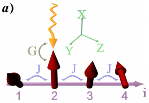
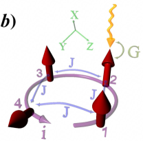
Figure 1: Theorist’s rendering of open (a), or cyclic (b) configurations of four spin chains. The wiggle line represents the photon.

For the calculations we choose a basis set of states by first ordering the field states, ($|0\rangle,|1\rangle),$ where $0\textrm{ and }1$ stand for the number of photons, then for each spin site we have the spin states ($|\uparrow\rangle,|\downarrow\rangle$). This gives a set of $2^{N+1}$ basis states. The spin operators in this basis are expressed through the Pauli matrices by the standard relations, $S^{x,y,z}=\tfrac{1}{2}\hbar\sigma^{x,y,z}$. Since the spin-spin term $S_{i}^{x}S_{i+1}^{x}+S_{i}^{y}S_{i+1}^{y}$ can be written as $\tfrac{1}{2}(S_{i}^{+}S_{i+1}^{-}+S_{i}^{-}S_{i+1}^{+})$, it useful to define additionally $\sigma^{\pm}=\tfrac{1}{2}\left(\sigma^{x}\pm\textrm{i}\sigma^{y}\right)$, so by definition $S^{\pm}=\hbar\sigma^{\pm}$. To summarize for spin $\tfrac{1}{2}$ we have the expressions:

$$\sigma^{x}=\begin{pmatrix}0&1\\ 1&0\end{pmatrix},\;\;\sigma^{y}=\begin{pmatrix}0&\textrm{-i}\\ \textrm{i}&0\end{pmatrix},\;\;\sigma^{z}=\begin{pmatrix}1&0\\ 0&-1\end{pmatrix},\;\;\textrm{ and }\ \ \ \mathbb{I}=\begin{pmatrix}1&0\\ 0&1\end{pmatrix},$$ (2a)

$$|\uparrow\rangle=\begin{pmatrix}1\\ 0\end{pmatrix},\;\;|\downarrow\rangle=\begin{pmatrix}0\\ 1\end{pmatrix},\;\;$$ (2b)

and for the photon we have

$$a=\begin{pmatrix}0&1\\ 0&0\end{pmatrix},\;\;a^{{\dagger}}=\begin{pmatrix}0&0\\ 1&0\end{pmatrix},\;\;$$ (3a)

$$|0\rangle=\begin{pmatrix}1\\ 0\end{pmatrix},\;\;|1\rangle=\begin{pmatrix}0\\ 1\end{pmatrix}.$$ (3b)

Since the field and the spin operators on different sites act independently, the matrix form for the subscripted $\sigma_{i}$ is a tensor product of $N+1$, $2\times 2$ matrices as follows (e.g. $\S$2.5 of [16]):

$$\sigma_{i}^{x}=\underbrace{\mathbb{I}}_{\mathrm{Field\ mode}}\otimes\underbrace{\mathbb{I}\otimes\mathbb{I}\otimes\cdots\otimes\mathbb{I}}_{i-1\ \mathrm{terms}}\otimes\underbrace{\sigma^{x}}_{i\mathrm{th\ spin}}\otimes\underbrace{\mathbb{I}\otimes\mathbb{I}\otimes\cdots\otimes\mathbb{I}}_{N-i\ \mathrm{terms}},$$ (4)

and similarly for $\sigma_{i}^{y},\sigma_{i}^{\pm}.$ This gives for the field-spin parts of the Hamiltonian:

$$a^{\dagger}\sigma_{j}^{y}=\underbrace{a^{\dagger}}_{\mathrm{Field\ mode}}\otimes\underbrace{\mathbb{I}\otimes\mathbb{I}\otimes...\otimes\mathbb{I}}_{j-1\ \mathrm{terms}}\otimes\underbrace{\sigma^{y}}_{j\mathrm{th\ spin}}\otimes\underbrace{\mathbb{I}\otimes\mathbb{I}\otimes...\otimes\mathbb{I}}_{N-j\ \mathrm{terms}},$$ (5)

and for the spin-spin terms:

$$\sigma_{i}^{x}\sigma_{j}^{y}=\underbrace{\mathbb{I}}_{\mathrm{Field\ mode}}\otimes\underbrace{\mathbb{I}\otimes\cdots\otimes\mathbb{I}}_{i-1\mathrm{\ terms}}\otimes\underbrace{\sigma^{x}}_{i{th\ \mathrm{spin}}}\otimes\underbrace{\mathbb{I}\otimes\cdots\otimes\mathbb{I}}_{j-i-1\mathrm{\ terms}}\otimes\underbrace{\sigma^{y}}_{\mathrm{j{th\ spin}}}\otimes\underbrace{\mathbb{I}\otimes\cdots\otimes\mathbb{I}}_{N-j\mathrm{\ terms}}.$$ (6)

3 The energy spectra for 4 spin chain

We diagonalize equation (1), expressed in matrix form using (5-6) for the case of four spins, $N=4,$ to obtain the exact solutions for the energy levels. To this end we solve the characteristic equation for $E$ i.e.

$$\det\left(\widehat{H}-E\;\mathbb{I}_{32\times 32}\right)=0.$$

The Hamiltonian is a $32\times 32$ matrix, and accordingly, there are 32 (some multiply degenerate) energy levels, which we found with help of a computer algebra system. For the open spin chain, the results depend on whether the photon falls on the first or the second spin, while the addition of the cyclic interactions term would appear to make this distinction irrelevant for the closed chain, as the results show as well. In order to check the computer derived formulae, it is useful to compare the limit $J=0$ with the known solutions of the two level Jaynes-Cummings model, which are $\pm G$ and $0$ in units of $\hbar$.

3.1 Open chain – edge coupled photon

The spectrum in this case consists of 9 distinct energy branches shown in Figure 2. The analytic expressions , where the superscripts $D,Q,$ or $O$ stand for the degeneracy of each level $2,4,$ or $8$ times, listed in decreasing order at $G=0$ are:

$$E^{D}_{1}(G,J) =\sqrt{G^{2}+3J^{2}+2\sqrt{2G^{2}J^{2}+J^{4}}},$$ (7a)

$$E^{Q}_{2}(G,J) =\frac{\sqrt{G^{2}+3J^{2}+\sqrt{G^{4}-2G^{2}J^{2}+5J^{4}}}}{\sqrt{2}},$$ (7b)

$$E^{D}_{3}(G,J) =\sqrt{G^{2}+3J^{2}-2\sqrt{2G^{2}J^{2}+J^{4}}},$$ (7c)

$$E^{Q}_{4}(G,J) =\frac{\sqrt{G^{2}+3J^{2}-\sqrt{G^{4}-2G^{2}J^{2}+5J^{4}}}}{\sqrt{2}},$$ (7d)

$$E^{O}_{5}(G,J) =0,$$ (7e)

and $E^{Q}_{6}=-E^{Q}_{4},\;E^{D}_{7}=-E^{D}_{3},\;E^{Q}_{8}=-E^{Q}_{2},\;E^{D}_{9}=-E^{D}_{1}.$ The (at least) double degeneracy of the levels follows from the Kramers theorem (we do not have an explicit magnetic field in the Hamiltonian), where the photon acts as an additional spin in the chain for the purposes of the theorem (see e.g. $\S$ 60 of [17]). To better show the behavior of the levels with predominantly light-spin interaction ($J\ll G$) or predominantly spin-spin interaction ($G\ll J$) we have used the substitution $G=C\cos\varphi,J=C\sin\varphi,$ where in the Figure 2(b), $C=1.$ With this notation, when $\varphi\in(-\tfrac{\pi}{2},0)$ the chain is an AFM chain, and when $\varphi\in(0,\tfrac{\pi}{2})$ it is a FM chain. Additionally shown is the region $\varphi>\tfrac{\pi}{2},$ where $G$ formally takes negative values. This would mean an overall change of the sign of the Hamiltonian, and accordingly, we see an energy spectrum that consists of the same levels, just arranged with opposite signs, so solid lines go to the corresponding solid lines at the line at $\varphi=\tfrac{\pi}{2}$.

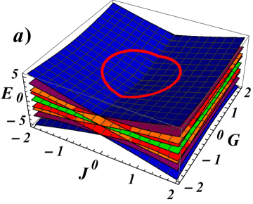
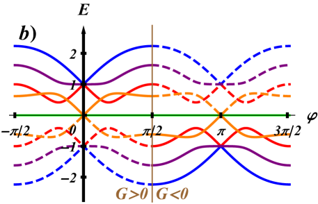
Figure 2: (Color online) The energy spectra given by equations (7) for a 4 spin chain coupled to a photon at the edge of the chain. (a) Energy surfaces at various finite strengths $G$ and $J.$ (b) The cross sections of the energy surfaces at the red (solid line) circle shown in (a). See text for further discussion of the notations and the symmetries of the spectrum. Close to $\varphi=0,$ $J\ll G$, and close to $\varphi=\tfrac{\pi}{2},$ $G\ll J.$

3.2 Open chain – photon coupled to the second spin in the chain

Due to the extra neighbor to the spin impacted by light, the qualitative change in the spectrum, is that the quadruply degenerate bands in (7) split into doubly degenerate bands, and thus all levels, except the zero energy, are now doubly degenerate. The eigenvalues in explicit form look rather cumbersome, so we first give the characteristic equation. It could be written in factored form as:

$$\det\left(\widehat{H}-E\;\mathbb{I}_{32\times 32}\right) =E^{8}\left[E^{4}-(G^{2}+3J^{2})E^{2}+(G^{2}+J^{2})J^{2}\right]^{2}$$

$$\quad\times\left\{E^{8}-(3G^{2}+9J^{2})E^{6}+(3G^{4}+15G^{2}J^{2}+24J^{4})E^{4}\right.$$

$$\qquad-(G^{6}+7G^{4}J^{2}+23G^{2}J^{4}+21J^{6})E^{2}+G^{6}J^{2}+7G^{4}J^{4}$$

$$\qquad+\left.3G^{2}J^{6}+5J^{8}\right\}^{2}$$

$$=0.$$ (8)

The solutions of this equation are shown in Figure 3, and there are 6 branches in the upper half-plane, with 13 overall distinct solutions. From the first factor we get the octuply degenerate zero level,

$$E^{O}(G,J)=0,$$ (9)

from the second factor (expression in the square brakets) and the third factor (curly brackets) the remaining doubly degenerated eigenvalues. The expressions from the second factor:

$$E_{a,b}^{D}(G,J)=-E_{c,d}^{D}(G,J)=\frac{\sqrt{G^{2}+3J^{2}\pm\sqrt{G^{4}+2G^{2}J^{2}+5J^{4}}}}{\sqrt{2}},$$ (10)

look similar to the $E^{Q}_{2,4}(G,J)$ (and $E^{Q}_{6,8}(G,J)$) in equation (7), with the only change in sign in the term in the second square root: $-2G^{2}J^{2}\rightarrow+2G^{2}J^{2}.$ The expressions for those from the third factor (the eight remaining lines on the figure), as solutions of fourth order equation for $E^{2},$ look involved and we only note that the topmost band, which is given by one of the roots of this fourth order equation, looks similar, with a slight decrease in the initial slope at $J\rightarrow 0,$ to the topmost band $E^{D}_{1}$ in (7).

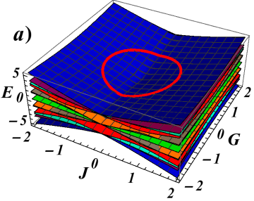
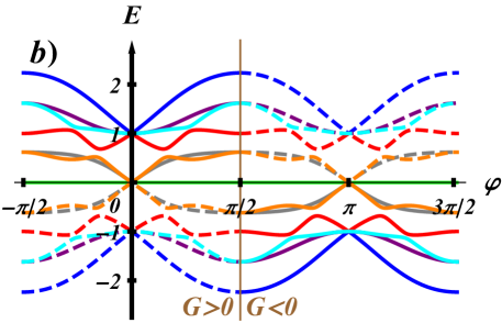
Figure 3: (Color online) The energy spectra given by equations (8) for a 4 spin chain coupled to a photon at second spin in the chain. Notations are similar to Figure 2.

3.3 Closed chain

The 4-spin cyclic configuration is described by the following characteristic equation:

$$\det\left(\widehat{H}_{C}-E\;\mathbb{I}_{32\times 32}\right) =E^{8}\left(E^{2}-G^{2}\right)^{2}\left[E^{4}-(G^{2}+4J^{2})E^{2}+2G^{2}J^{2}\right]^{2}$$

$$\quad\times\left\{E^{6}-(2G^{2}+12J^{2})E^{4}+(G^{4}+6G^{2}J^{2}+32J^{4})E^{2}-2G^{4}J^{2}-8G^{2}J^{4}\right\}^{2}$$

$$=0,$$ (11)

whose 13 distinct solutions are shown in the Figure 4. $\widehat{H}_{C}$ compared to (1), has an additional spin-spin interaction term between the spins on sites $N$ and $1$; thus closing the chain. Except for the octuply degenerate zero level,

$$E^{O}(G,J)=0,$$ (12)

the energy spectrum consists of doubly degenerate levels. The second factor gives:

$$E_{A,B}^{D}(G,J)=\pm G,$$ (13)

which is independent of $J$. In Figure 4(b) it appears as a cosine (cyan) line. We have checked, that for a 3-spin chain there also is an energy level that is linear in G, but has an additional, also linear, dependence on $J.$ Here such levels come from a mixture of different basic spin configurations, for which the magnetic part of the Hamiltonian (1) produces canceling contributions. The third, quadratic in $E^{2},$ factor gives:

$$E^{D}_{a,b}(G,J)=-E^{D}_{c,d}(G,J)=\frac{\sqrt{G^{2}+4J^{2}\pm\sqrt{G^{4}+16J^{4}}}}{\sqrt{2}}.$$ (14)

The last factor, curly brackets in (11), is cubic in $E^{2}$ and gives the remaining 12 roots (counting the degeneracy), or 6 lines on the figure, and the topmost band is one of these roots. The explicit formulae are again somewhat cumbersome, and we skip writing them explicitly.

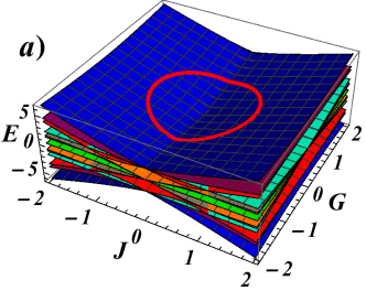
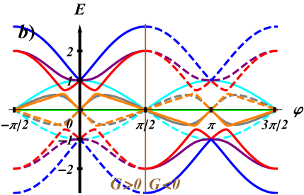
Figure 4: (Color online) The energy spectra from equation (11) for a 4 spin cyclic chain coupled to a photon. Notations are similar to Figure 2.

4 Conclusions

In this report we have discussed some analytical results of applying the Jaynes-Cummings model to an XY- AFM or FM spin $\tfrac{1}{2}$ chain. Because we limited ourselves to a single mode photon field, the resulting Hamiltonian in matrix form resembles the case of a pure spin chain with one extra spin site inducing anisotropy. Nevertheless the light-spin interaction term does bring a novel effect: it does not commute with the total spin $S_{z}^{\mathrm{total}}=\tfrac{1}{2}\sum_{i=1}^{N}\sigma^{z}_{i}.$ This means that the eigenstates of the XY-Jaynes-Cummings Hamiltonian consist of some mixtures of the product basis states, which have definite spin moment value. For that reason only for $G=0$ ($\varphi=\tfrac{\pi}{2}$ point in figures 2, 3, 4) it is possible to assign definite spin moment to the energy levels. As can be seen from the equations, the 4-spin chain seems to be the limit for the analytical formulae, since more sites would require solving polynomial equations of more than 5-th power, which may not have a closed form. It was possible to obtain numerical data for the energy levels of a chain made of more than 4 spins, this would be reported in some future work [18].

This work was supported by EU FP7 INERA project grant agreement number 316309. We thank N. Tonchev for bringing our attention to [19].

References

References

- [1] Jaynes E and Cummings F 1963 Proceedings of the IEEE 51 89–109
- [2] Vogel W and de Matos Filho R L 1995 Phys. Rev. A 52 4214–4217
- [3] You J Q and Nori F 2003 Phys. Rev. B 68 064509
- [4] Rempe G, Walther H and Klein N 1987 Phys. Rev. Lett. 58 353–356
- [5] Dodonov A V, Mizrahi S S and Dodonov V V 2006 Phys. Rev. A 74 033823
- [6] Gerry C and Knight P 2004 Introductory quantum optics (Cambridge: Cambridge University Press)
- [7] Scully M O and Zubairy M S 1997 Quantum Optics (Cambridge: Cambridge University Press)
- [8] Dziarmaga J 2005 Phys. Rev. Lett. 95 245701
- [9] Arnesen M C, Bose S and Vedral V 2001 Phys. Rev. Lett. 87 017901
- [10] Batle J and Casas M 2010 Phys. Rev. A 82 062101
- [11] Maucourt J and Grempel D R 1998 Phys. Rev. Lett. 80 770–773
- [12] Wang X 2001 Phys. Rev. A 64 012313
- [13] Wang Y K and Hioe F T 1973 Phys. Rev. A 7 831–836
- [14] Takayoshi S, Aoki H and Oka T 2014 Phys. Rev. B 90 085150
- [15] The invariant terms in the total Hamiltonian have been rotated away with a unitary transformation, cf. [19]
- [16] Rumer Y and Fet A 1970 The theory of unitary symmetry (Moscow: Nauka)
- [17] Landau L D and Lifshitz E M 1989 Quantum Mechanics: Non-relativistic Theory (Vol 3) 3rd ed (Oxford: Pergamon Press)
- [18] Tonchev H, Donkov A A and Chamati H (in preparation)
- [19] Juárez-Amaro R, Zúñiga-Segundo A and Moya-Cessa H M 2015 Appl. Math. Inf. Sci. 9 299–303