MapReduce and Streaming Algorithms for Diversity Maximization in Metric Spaces of Bounded Doubling Dimension

Abstract

Given a dataset of points in a metric space and an integer $k$, a diversity maximization problem requires determining a subset of $k$ points maximizing some diversity objective measure, e.g., the minimum or the average distance between two points in the subset. Diversity maximization is computationally hard, hence only approximate solutions can be hoped for. Although its applications are mainly in massive data analysis, most of the past research on diversity maximization focused on the sequential setting. In this work we present space and pass/round-efficient diversity maximization algorithms for the Streaming and MapReduce models and analyze their approximation guarantees for the relevant class of metric spaces of bounded doubling dimension. Like other approaches in the literature, our algorithms rely on the determination of high-quality core-sets, i.e., (much) smaller subsets of the input which contain good approximations to the optimal solution for the whole input. For a variety of diversity objective functions, our algorithms attain an $(\alpha+\varepsilon)$-approximation ratio, for any constant $\varepsilon>0$, where $\alpha$ is the best approximation ratio achieved by a polynomial-time, linear-space sequential algorithm for the same diversity objective. This improves substantially over the approximation ratios attainable in Streaming and MapReduce by state-of-the-art algorithms for general metric spaces. We provide extensive experimental evidence of the effectiveness of our algorithms on both real world and synthetic datasets, scaling up to over a billion points.

1 Introduction

Diversity maximization is a fundamental primitive in massive data analysis, which provides a succinct summary of a dataset while preserving the diversity of the data [1, 27, 33, 34]. This summary can be presented visually to the user or can be used as a core for further processing of the dataset. In this paper we present novel efficient algorithms for diversity maximization in popular computation models for massive data processing, namely Streaming and MapReduce.

Diversity Measures and their Applications:

Given a dataset of points in a metric space and a constant $k$, a solution to the diversity maximization problem is a subset of $k$ points that maximizes some diversity objective measure defined in terms of the distances between the points.

Combinations of relevance ranking and diversity maximization have been explored in a variety of applications, including web search [5], e-commerce [7], recommendation systems [35], aggregate websites [28] and query-result navigation [14] (see [31, 1, 23] for further references on the applications of diversity maximization). The common problem in all these applications is that even after filtering and ranking for relevance, the output set is often too large to be presented to the user. A practical solution is to present a diverse subset of the results so the user can evaluate the variety of options and possibly refine the search.

There are a number of ways to formulate the goal of finding a set of $k$ points which are as diverse, or as far as possible from each other. Conceptually, a $k$-diversity maximization problem can be formulated in terms of a specific graph-theoretic measure defined on sets of $k$ points, seen as the nodes of a clique where each edge is weighted with the distance between its endpoints [12]. Several diversity measures are defined in Table 1. While the most appropriate ones in the context of web search, e-commerce, aggregator systems and query results navigation are the remote-edge and the remote-clique measures [17, 1], the results in this paper also extend to the other measures in the table, which have important applications in analyzing network performance, locating strategic facilities or noncompeting franchises, or determining initial solutions for iterative clustering algorithms or heuristics for hard optimization problems such as TSP [21, 12, 31]. We include all of these measures here to demonstrate the versatility of our approach to a variety of diversity criteria. We want to stress that different measures characterize the diversity of a set in a different fashion: indeed, an optimal solution with respect to one measure is not necessarily optimal with respect to another measure.

Distance Metric:

All the diversity criteria listed in Table 1 are known to be NP-hard for general metric spaces. Following a number of recent works [2, 15, 25, 19, 8, 9], we parameterize our results in terms of the doubling dimension of the metric space. Recall that a metric space has doubling dimension $D$ if any ball of radius $r$ can be covered by at most $2^{D}$ balls of radius $r/2$. While our methods yield provably tight bounds in spaces of bounded doubling dimension (e.g., any bounded dimension Euclidian space) they have the ability of providing good approximations in more general spaces based on important practical distance functions such as the cosine distance in web search [5] and the dissimilarity (Jaccard) distance in database queries [26].

Massive Data Computation Models:

Since the applications of diversity maximization are mostly in the realm of massive data analysis, it is important to develop efficient algorithms for computational settings that can handle very large datasets.

Problem	Diversity measure	Sequential approximation
remote-edge	$\min_{p,q\in S}d(p,q)$	2 (2) [32]
remote-clique	$\sum_{p,q\in S}d(p,q)$	2 ($-$) [22]
remote-star	$\min_{c\in S}\sum_{q\in S\setminus\{c\}}d(c,q)$	2 ($-$) [12]
remote-bipartition	$\min_{Q\subset S,|Q|=\lfloor|S|/2\rfloor}\sum_{q\in Q,z\in S\setminus Q}d(q,z)$	3 ($-$) [12]
remote-tree	$w(\operatorname{MST}(S))$	4 (2) [21]
remote-cycle	$w(\operatorname{TSP}(S))$	3 (2) [21]

Table 1: Diversity measures considered in this paper. $w(\operatorname{MST}(S))$ (resp., $w(\operatorname{TSP}(S))$) denotes the minimum weight of a spanning tree (resp., Hamiltonian cycle) of the complete graph whose nodes are the points of $S$ and whose edge weights are the pairwise distances among the points. The last column lists the best known approximation factor, the lower bound under the hypothesis $P\neq NP$ (in parentheses), and the related references.

The Streaming and MapReduce models are widely recognized as suitable computational frameworks for big-data processing. The Streaming model [30] copes with large data volumes through an on-the-fly computation on the streamlined dataset, storing only very limited information in the process, while the MapReduce model [24, 29] enables the handling of large datasets through the massive availability of resource-limited processing elements working in parallel. The major challenge in both models is devising strategies which work under the constraint that the number of data items that a single processor can access simultaneously is substantially limited.

Related work.

Diversity maximization has been studied in the literature under different names (e.g., $p$-Dispersion, Max-Min Facility Dispersion, etc.). An extensive account of the existing formulations is provided in [12]. All of these problems are known to be NP-hard, and several sequential approximation algorithms have been proposed. Table 1 summarizes the best known results for general metric spaces. There are also some specialized results for spaces with bounded doubling dimension: for the remote-clique problem, a polynomial-time $(\sqrt{2}+\varepsilon)$-approximation algorithm on the Euclidean plane, and a polynomial-time $(1+\varepsilon)$-approximation algorithm on $d$-dimensional spaces with rectilinear distances, for any positive constants $\varepsilon>0$ and $d$, are presented in [16]. In [21] it is shown that a natural greedy algorithm attains a $2.309$ approximation factor on the Euclidean plane for remote-tree. Recently, the remote-clique problem has been considered under matroid constraints [1, 11], which generalize the cardinality constraints considered in previous literature.

In recent years, the notion of (composable) core-set has been introduced as a key tool for the efficient solution of optimization problems on large datasets. A core-set [3], with respect to a given computational objective, is a (small) subset of the entire dataset which contains a good approximation to the optimal solution for the entire dataset. A composable core-set [23] is a collection of core-sets, one for each subset in an arbitrary partition of the dataset, such that the union of these core-sets contains a good core-set for the entire dataset. The approximation factor attained by a (composable) core-set is defined as the ratio between the value of the global optimal solution and the value of the optimal solution on the (composable) core-set. For the problems listed in Table 1, composable core-sets with constant approximation factors have been devised in [23, 4] (see Table 2). As observed in [23], (composable) core-sets may become key ingredients for developing efficient algorithms for the MapReduce and Streaming frameworks, where the memory available for a processor’s local operations is typically much smaller than the overall input size.

In recent years, the characterization of data through the doubling dimension of the space it belongs to has been increasingly used for algorithm design and analysis in a number of contexts, including clustering [2], nearest neighbour search [15], routing [25], machine learning [19], and graph analytics [8, 9].

	Previous [23, 4]	Our results
	General metric spaces	Bounded doubling dimension
remote-edge	$3$	$1+\varepsilon$
remote-clique	$6+\varepsilon$	$1+\varepsilon$
remote-star	$12$	$1+\varepsilon$
remote-bipartition	$18$	$1+\varepsilon$
remote-tree	$4$	$1+\varepsilon$
remote-cycle	$3$	$1+\varepsilon$

Table 2: Approximation factors of the composable core-sets computed by our algorithm, compared with previous approaches.

Our contribution.

In this paper we develop efficient algorithms for diversity maximization in the Streaming and MapReduce models. At the heart of our algorithms are novel constructions of (composable) core-sets. In contrast to [23, 4], where different constructions are devised for each diversity objective, we provide a unique construction technique for all of the six objective functions. While our approach is applicable to general metric spaces, on spaces of bounded doubling dimension, our (composable) core-sets feature a $1+\varepsilon$ approximation factor, for any fixed $0<\varepsilon\leq 1$, for all of the six diversity objectives, with the core-set size increasing as a function of $1/\varepsilon$. The approximation factor is significantly better than the ones attained by the known composable core-sets in general metric spaces, which are reported in Table 2 for comparison.

Once a core-set (possibly obtained as the union of composable core-sets) is extracted from the data, the best known sequential approximation algorithm can be run on it to derive the final solution. The resulting approximation ratio attained in this fashion combines two sources of error: (1) the approximation loss in replacing the entire dataset with a core-set; and (2) the approximation factor of the sequential approximation algorithm executed on the core-set. On metric spaces of bounded doubling dimension the combined approximation ratio attained by our algorithms for any of the six diversity objective functions considered in the paper is bounded by $(\alpha+\varepsilon)$, for any constant $0<\varepsilon\leq 1$, where $\alpha$ the is best approximation ratio achieved by a polynomial-time, linear-space sequential algorithm for the same maximum diversity criterion.

Our algorithms require only one pass over the data, in the streaming setting, and only two rounds in MapReduce. To the best of our knowledge, for all six diversity problems, our streaming algorithms are the first ones that yield approximation ratios close to those of the best sequential algorithms using space independent of input stream size. Also, we remark that the parallel strategy at the base of the MapReduce algorithms can be effectively ported to other models of parallel computation.

Finally, we provide experimental evidence of the practical relevance of our algorithms on both synthetic and real-world datasets. In particular, we show that higher accuracy is achievable by increasing the size of the core-sets, and that the MapReduce algorithm is considerably faster (up to three orders of magnitude) than its state-of-the-art competitors. Also, we provide evidence that the proposed approach is highly scalable. We want to remark that our work provides the first substantial experimental study on the performance of diversity maximization algorithms on large instances of up to billions of data points.

The rest of the paper is organized as follows. In Section 2, we introduce some fundamental concepts and useful notations. In Section 3, we identify sufficient conditions for a subset of points to be a core-set with provable approximation guarantees. These properties are then crucially exploited by the streaming and MapReduce algorithms described in Sections 4 and 5, respectively. Section 6 discusses how the higher memory requirements of four of the six diversity problems can be reduced, while Section 7 reports on the results of the experiments.

2 Preliminaries

Let $({\cal D},d)$ be a metric space. The distance between two points $u,v\in{\cal D}$ is denoted by $d(u,v)$. Moreover, we let $d(p,S)=\min_{q\in S}d(p,q)$ denote the minimum distance between a point $p\in{\cal D}$ and an element of a set $S\subseteq{\cal D}$. Also, for a point $p\in{\cal D}$, the ball of radius $r$ centered at $p$ is the set of all points in ${\cal D}$ at distance at most $r$ from $p$. The doubling dimension of a space is the smallest $D$ such that any ball of radius $r$ is covered by at most $2^{D}$ balls of radius $r/2$ [20]. As an immediate consequence, for any $0<\varepsilon\leq 1$, any ball of radius $r$ can be covered by at most $(1/\varepsilon)^{D}$ balls of radius $\varepsilon r$. For ease of presentation, in this paper we concentrate on metric spaces of constant doubling dimension $D$, although the results can be immediately extended to nonconstant $D$ by suitably adjusting the ranges of variability of the parameters involved. Several relevant metric spaces have constant doubling dimension, a notable case being Euclidean space of constant dimension $D$, which has doubling dimension $O\left(D\right)$ [20].

Let $\operatorname{div}:2^{\cal D}\rightarrow\mathbb{R}$ be a diversity function that maps a set $S\subset{\cal D}$ to some nonegative real number. In this paper, we will consider the instantiations of function $\operatorname{div}$ listed in Table 1, which were introduced and studied in [12, 23, 4]. For a specific diversity function $\operatorname{div}$, a set $S\subset{\cal D}$ of size $n$ and a positive integer $k\leq n$, the goal of the diversity maximization problem is to find some subset $S^{\prime}\subseteq S$ of size $k$ that maximizes the value $\operatorname{div}(S^{\prime})$. In the following, we refer to the $k$-diversity of $S$ as

$$\operatorname{div}_{k}(S)=\max_{S^{\prime}\subseteq S,|S^{\prime}|=k}\operatorname{div}(S^{\prime})$$

The notion of core-set [3] captures the idea of a small set of points that approximates some property of a larger set.

Definition 1.

Let $\operatorname{div}(\cdot)$ be a diversity function, $k$ be a positive integer, and $\beta\geq 1$. A set $T\subseteq S$, with $|T|\geq k$, is a $\beta$-core-set for $S$ if

$$\operatorname{div}_{k}(T)\geq\frac{1}{\beta}\operatorname{div}_{k}(S)$$

In [23, 4], the concept of core-set is extended so that, given an arbitrary partition of the input set, the union of the core-sets of each subset in the partition is a core-set for the entire input set.

Definition 2.

Let $\operatorname{div}(\cdot)$ be a diversity function, $k$ be a positive integer, and $\beta\geq 1$. A function $c(S)$ that maps $S\subset{\cal D}$ to one of its subsets computes a $\beta$-composable core-set w.r.t. $\operatorname{div}$ if, for any collection of disjoint sets $S_{1},\dots,S_{\ell}\subset{\cal D}$ with $|S_{i}|\geq k$, we have

$$\operatorname{div}_{k}\left(\bigcup_{i=1}^{\ell}c(S_{i})\right)\geq\frac{1}{\beta}\operatorname{div}_{k}\left(\bigcup_{i=1}^{\ell}S_{i}\right)$$

Consider a set $S\subseteq{\cal D}$ and a subset $T\subseteq S$. We define the range of $T$ as $r_{T}=\max_{p\in S\setminus T}d(p,T)$, and the farness of $T$ as $\rho_{T}=\min_{c\in T}\{d(c,T\setminus\{c\})\}$. Moreover, we define the optimal range $r_{k}^{*}$ for $S$ w.r.t. $k$ to be the minimum range of a subset of $k$ points of $S$. Similarly, we define the optimal farness $\rho_{k}^{*}$ for $S$ w.r.t. $k$ to be the maximum farness of a subset of $k$ points of $S$. Observe that $\rho_{k}^{*}$ is also the value of the optimal solution to the remote-edge problem.

3 Core-set characterization

In this section we identify some properties that, when exhibited by a set of points, guarantee that the set is a $(1+\varepsilon)$-core-set for the diversity problems listed in Table 1. In the subsequent sections we will show how core-sets with these properties can be obtained in the streaming and MapReduce settings. In fact, when we discuss the MapReduce setting, we will also show that these properties also yield composable core-sets featuring tighter approximation factors than existing ones, for spaces with bounded doubling dimension.

First, we need to establish a fundamental relation between the optimal range $r_{k}^{*}$ and the optimal farness $\rho_{k}^{*}$ for a set $S$. To this purpose, we observe that the classical greedy approximation algorithm proposed in [18] for finding a subset of minimum range ($k$-center problem), gives in fact a good approximation to both measures. We refer to this algorithm as GMM. Consider a set of points $S$ and a positive integer $k<|S|$. Let $T=\mbox{\sc GMM}(S,k)$ be the subset of $k$ points returned by the algorithm for this instance. The algorithm initializes $T$ with an arbitrary point $a\in S$. Then, greedily, it adds to $T$ the point of $S\setminus T$ which maximizes the distance from the already selected points, until $T$ has size $k$. It is known that the returned set $T$ is such that $r_{T}\leq 2r_{k}^{*}$ [18] and it is easily seen that $r_{T}\leq\rho_{T}$ (referred to as anticover property). This immediately implies the following fundamental relation.

Fact 1.

Given a set $S$ and $k>0$, we have $r_{k}^{*}\leq\rho_{k}^{*}$.

Let $S$ be a set belonging to a metric space of doubling dimension $D$. In what follows, $\operatorname{div}(\cdot)$ denotes the diversity function of the problem under consideration, and $O$ denotes an optimal solution to the problem with respect to instance $S$. Consider a subset $T\subseteq S$. Intuitively, $T$ is a good core-set for some diversity measure on $S$, if for each point of the optimal solution $O$ it contains a point sufficiently close to it. We formalize this intuition by suitably adapting the notion of proxy function introduced in [23]. Given a core-set $T\subseteq S$, we aim at defining a function $p:O\rightarrow T$ such that the distance between $o$ and $p(o)$ is bounded, for any $o\in O$. For some problems this function will be required to be injective, whereas for, some others, injectivity will not be needed. We begin by studying the remote-edge and the remote-cycle problem.

Lemma 1.

For any given $\varepsilon>0$, let $\varepsilon^{\prime}$ be such that $(1-\varepsilon^{\prime})=1/(1+\varepsilon)$. A set $T\subseteq S$ is a $(1+\varepsilon)$-core-set for the remote-edge and the remote-cycle problems if $|T|\geq k$ and there is a function $p:O\rightarrow T$ such that, for any $o\in O$, $d(o,p(o))\leq(\varepsilon^{\prime}/2)\rho_{k}^{*}$.

Proof.

Consider the remote-edge problem first, and observe that $\operatorname{div}_{k}(T)\leq\operatorname{div}(O)=\rho_{k}^{*}$. By applying the triangle inequality and the stated property of the proxy function $p$ we get

$$\operatorname{div}_{k}(T) \geq\min_{o_{1},o_{2}\in O}d(p(o_{1}),p(o_{2}))\geq\min_{o_{1},o_{2}\in O}\{d(o_{1},o_{2})-d(o_{1},p(o_{1}))-d(o_{2},p(o_{2}))\}$$

$$\geq\min_{o_{1},o_{2}\in O}d(o_{1},o_{2})-\varepsilon^{\prime}\rho_{k}^{*}=\operatorname{div}(O)(1-\varepsilon^{\prime})=\operatorname{div}(O)/(1+\varepsilon)$$

Note that $p(\cdot)$ does not need to be injective: in fact, if two points of the optimal solution are mapped into the same proxy, the first inequality trivially holds, its right hand side being zero.

Consider now the remote-cycle problem. Note that $\operatorname{div}_{k}(T)\leq\operatorname{div}(O)$. Let $\bar{\rho}=\operatorname{div}(O)/k$ and observe that $\rho_{k}^{*}\leq\bar{\rho}$. Let $P=\{p(o):o\in O\}\subseteq T$ be the image of the proxy function. Following the argument given in [23, 4], consider $\operatorname{TSP}(P)$, an optimal tour on $P$. We build a weighted graph $G$ whose vertex set is $O\cup P$ and whose edges are those induced by $\operatorname{TSP}(P)$ plus two copies of edge $(o,p(o))$, for each $o\in O$. The weight of an edge $(u,v)$ is $d(u,v)$. Clearly, the resulting graph $G$ is connected and all its vertices have even degree, therefore it admits an Euler tour $T_{E}$ of its edges. From $T_{E}$ we obtain a cycle $C$ of $O$ by shortcutting all nodes that are not in $O$. By repeated applications of the triangle inequality during shortcutting and the fact that $d(o,p(o))\leq(\varepsilon^{\prime}/2)\bar{\rho}$, we obtain:

$$w(\operatorname{TSP}(O)) \leq w(C)\leq w(T_{E})\leq w(\operatorname{TSP}(P))+k\varepsilon^{\prime}\bar{\rho}$$

$$\leq\operatorname{div}_{k}(T)+\varepsilon^{\prime}\operatorname{div}(O)$$

Therefore, $\operatorname{div}(O)\leq\operatorname{div}_{k}(T)/(1-\varepsilon^{\prime})=\operatorname{div}_{k}(T)(1+\varepsilon)$. As in the case of the remote-edge problem, the injectivity of $p(\cdot)$ is not necessary. ∎

Note that the proof of the above lemma does not require $p(\cdot)$ to be injective. Instead, injectivity is required for the remote-clique, remote-star, remote-bipartition, and remote-tree problems, which are considered next.

Lemma 2.

For a given $\varepsilon>0$, let $\varepsilon^{\prime}$ be such that $1-\varepsilon^{\prime}=1/(1+\varepsilon)$. A set $T\subseteq S$ is a $(1+\varepsilon)$-core-set for the remote-clique, remote-star, remote-bipartition, and remote-tree problems if $|T|\geq k$ and there is an injective function $p:O\rightarrow T$ such that, for any $o\in O$, $d(o,p(o))\leq(\varepsilon^{\prime}/2)\rho_{k}^{*}$.

Proof.

Observe that for each of the four problems it holds that $\operatorname{div}_{k}(T)\leq\operatorname{div}(O)$. Let us consider the remote-clique problem first, and define $\bar{\rho}=\operatorname{div}(O)/{k\choose 2}=\sum_{o_{1},o_{2}\in O}d(o_{1},o_{2})/{k\choose 2}$ Clearly, $\rho_{k}^{*}\leq\bar{\rho}$. By combining this observation with the triangle inequality we have

$$\operatorname{div}_{k}(T^{\prime}) \geq\sum_{o_{1},o_{2}\in O}d(p(o_{1}),p(o_{2}))\geq\sum_{o_{1},o_{2}\in O}\left[d(o_{1},o_{2})-d(o_{1},p(o_{1}))-d(o_{2},p(o_{2}))\right]$$

$$\geq\sum_{o_{1},o_{2}}d(o_{1},o_{2})-{k\choose 2}\varepsilon^{\prime}\bar{\rho}=\operatorname{div}(O)/(1+\varepsilon)$$

The injectivity of $p(\cdot)$ is needed in this case for the first inequality above to be true, since $k$ distinct proxies are needed to get a feasible solution. The argument for the other problems is virtually identical, and we omit it for brevity. ∎

4 Applications to data streams

In the Streaming model [30] one processor with a limited-size main memory is available for the computation. The input is provided as a continuous stream of items which is typically too large to fit in main memory, hence it must be processed on the fly within the limited memory budget. Streaming algorithms aim at performing as few passes as possible (ideally just one) over the input.

In [23], the authors propose the following use of composable core-sets to approximate diversity in the streaming model. The stream of $n$ input points is partitioned into $\sqrt{n/k}$ blocks of size $\sqrt{kn}$ each, and a core-set of size $k$ is computed from each block and kept in memory. At the end of the pass, the final solution is computed on the union of the core-sets, whose total size is $\sqrt{kn}$. In this section, we show that substantial savings (a space requirement independent of $n$) can be obtained by computing a single core-set from the entire stream through two suitable variants of the 8-approximation doubling algorithm for the $k$-center problem presented in [13], which are described below.

Let $k,k^{\prime}$ be two positive integers, with $k\leq k^{\prime}$. The first variant, dubbed SMM$(S,k,k^{\prime})$, works in phases and maintains in memory a set $T$ of at most $k^{\prime}+1$ points. Each Phase $i$ is associated with a distance threshold $d_{i}$, and is divided into a merge step and an update step. Phase 1 starts after an initialization in which the first $k^{\prime}+1$ points of the stream are added to $T$, and $d_{1}$ is set equal to $\min_{c\in T}d(c,T\setminus\{c\})$. At the beginning of Phase $i$, with $i\geq 1$, the following invariant holds. Let $S_{i}$ be the prefix of the stream processed so far. Then:

1. $\forall p\in S_{i}$, $d(p,T)\leq 2d_{i}$

2. $\forall t_{1},t_{2}\in T$, with $t_{1}\neq t_{2}$, we have $d(t_{1},t_{2})\geq d_{i}$

Observe that the invariant holds at the beginning of Phase 1. The merge step operates on a graph $G=(T,E)$ where there is an edge $(t_{1},t_{2})$ between two points $t_{1}\neq t_{2}\in T$ if $d(t_{1},t_{2})\leq 2d_{i}$. In this step, the algorithm seeks a maximal independent set $I\subseteq T$ of $G$, and sets $T=I$. The update step accepts new points from the stream. Let $p$ be one such new point. If $d(p,T)\leq 4d_{i}$, the algorithm discards $p$, otherwise it adds $p$ to $T$. The update step terminates when either the stream ends or the $(k^{\prime}+1)$-st point is added to $T$. At the end of the step, $d_{i+1}$ is set equal to $2d_{i}$. As shown in [13], at the end of the update step, the set $T$ and the threshold $d_{i+1}$ satisfy the above invariants for Phase $i+1$.

To be able to use SMM for computing a core-set for our diversity problems, we have to make sure that the set $T$ returned by the algorithm contains at least $k$ points. However, in the algorithm described above the last phase could end with $|T|<k$. To fix this situation, we modify the algorithm so to retain in memory, for the duration of each phase, the set $M$ of points that have been removed from $T$ during the merge step performed at the beginning of the phase. Consider the last phase. If at the end of the stream we have $|T|<k$, we can pick $k-|T|$ arbitrary nodes from $M$ and add them to $T$. Note that we can always do so because $M\cup I=k^{\prime}+1\geq k$, where $I$ is the independent set found during the last merge step.

Suppose that the input set $S$ belongs to a metric space with doubling dimension $D$. We have:

Lemma 3.

For any $0<\varepsilon^{\prime}\leq 1$, let $k^{\prime}=(32/\varepsilon^{\prime})^{D}\cdot k$, and let $T$ be the set of points returned by SMM$(S,k,k^{\prime})$. Then, given an arbitrary set $X\subseteq S$ with $|X|=k$, there exist a function $p:X\rightarrow T$ such that, for any $x\in X$, $d(x,p(x))\leq(\varepsilon^{\prime}/2)\rho^{*}_{k}$.

Proof.

Let $r_{k^{\prime}}^{*}$ to be the optimal range for $S$ w.r.t. $k^{\prime}$. Also, let $r_{T}=\max_{p\in S}d(p,T)$ be the range of $T$ and let $\rho_{k}^{*}$ be the optimal farness for $S$ w.r.t. $k$. Suppose that SMM$(S,k,k^{\prime})$ performs $\ell$ phases. It is immediate to see that $r_{T}\leq 4d_{\ell}$. As was proved in [13], $4d_{\ell}\leq 8r_{k^{\prime}}^{*}$, thus $r_{T}\leq 8r_{k^{\prime}}^{*}$. Consider now an optimal clustering of $S$ with $k$ centers and range $r_{k}^{*}$ and, for notational convenience, define $\varepsilon^{\prime\prime}=\varepsilon^{\prime}/32$. From the doubling dimension property, we know that there exist at most $k^{\prime}$ balls in the space (centered at nodes not necessarily in $S$) of radius at most $\varepsilon^{\prime\prime}r_{k}^{*}$ which contain all of the points in $S$. By choosing one arbitrary center in $S$ for each such ball, we obtain a feasible solution to the $k^{\prime}$-center problem for $S$ with range at most $2\varepsilon^{\prime\prime}r_{k}^{*}$. Consequently, $r_{k^{\prime}}^{*}\leq 2\varepsilon^{\prime\prime}r_{k}^{*}$. Hence, we have that $r_{T}\leq 8r_{k^{\prime}}^{*}\leq 16\varepsilon^{\prime\prime}r_{k}^{*}$. By Fact 1, we know that $r_{k}^{*}\leq\rho_{k}^{*}$. Therefore, we have $r_{T}\leq 16\varepsilon^{\prime\prime}\rho_{k}^{*}=(\varepsilon^{\prime}/2)\rho_{k}^{*}$. Given a set $X\subseteq S$ of size $k$, the desired proxy function $p(\cdot)$ is the one that maps each point $x\in X$ to the closest point in $T$. By the discussion above, we have that $d(x,p(x))\leq(\varepsilon^{\prime}/2)\rho_{k}^{*}$. ∎

For the diversity problems mentioned in Lemma 2, we need that for each point of an optimal solution the final core-set extracted from the data stream contains a distinct point very close to it. In what follows, we describe a variant of SMM, dubbed SMM-EXT, which ensures this property. Algorithm SMM-EXT proceeds as SMM but maintains for each $t\in T$ a set $E_{t}$ of at most $k$ delegate points close to $t$, including $t$ itself. More precisely, at the beginning of the algorithm, $T$ is initialized with the first $k^{\prime}+1$ points of the stream, as before, and $E_{t}$ is set equal to $\{t\}$, for each $t\in T$. In the merge step of Phase $i$, with $i\geq 1$, iteratively for each point $t_{1}$ not included in the independent set $I$, we determine an arbitrary point $t_{2}\in I$ such that $d(t_{1},t_{2})\leq 2d_{i}$ and let $E_{t_{2}}$ inherit $\max\{|E_{t_{1}}|,k-|E_{t_{2}}|\}$ points of $E_{t_{1}}$. Note that one such point $t_{2}$ must exist, otherwise $I$ would not be a maximal independent set. Also, note that a point $t_{2}\in I$ may inherit points from sets associated with different points not in $I$. Consider the update step of Phase $i$ and let $p$ be a new point from the stream. Let $t\in T$ be the point currently in $T$ which is closest to $p$. If $d(p,t)>4d_{i}$ we add it to $T$. If instead $d(p,t)\leq 4d_{i}$ and $|E_{t}|<k$, then we add $p$ to $E_{t}$, otherwise we discard it. Finally, we define $T^{\prime}=\bigcup_{t\in T}E_{t}$ to be the output of the algorithm, and observe that $T\subseteq T^{\prime}$.

Lemma 4.

For any $0<\varepsilon^{\prime}\leq 1$, let $k^{\prime}=(64/\varepsilon^{\prime})^{D}\cdot k$, and let $T^{\prime}$ be the set of points returned by SMM-EXT$(S,k,k^{\prime})$. Then, given an arbitrary set $X\subseteq S$ with $|X|=k$, there exist an injective function $p:X\rightarrow T^{\prime}$ such that, for any $x\in X$, $d(x,p(x))\leq(\varepsilon^{\prime}/2)\rho_{k}^{*}$.

Proof.

Let $r_{T^{\prime}}=\max_{p\in S}d(p,T^{\prime})$ be the range of $T^{\prime}$, and suppose that SMM$(S,k,k^{\prime})$ performs $\ell$ phases. By defining $\varepsilon^{\prime\prime}=\varepsilon^{\prime}/64$, and by reasoning as in the proof of Lemma 3 we can show that $r_{T^{\prime}}\leq 4d_{\ell}\leq 16\varepsilon^{\prime\prime}\rho_{k}^{*}$. Consider a point $x\in X$. If $x\in T^{\prime}$ then we define $p(x)=x$. Otherwise, suppose that $x$ is discarded during Phase $j$, for some $j$, because either in the merging or in the update step the set $E_{t}$ that was supposed to host it had already $k$ points. Let $T_{i}$ denote the set $T$ at the end of Phase $i$, for any $i\geq 1$. A simple inductive argument shows that at the end of each Phase $i$, with $j\leq i\leq\ell$ there is a point $t\in T_{i}$ such that $|E_{t}|=k$ and $d(x,t)\leq 4d_{i}$. In particular, there exists a point $t\in T_{\ell}$ such that $|E_{t}|=k$ and $d(x,t)\leq 4d_{\ell}\leq 16\varepsilon^{\prime\prime}\rho_{k}^{*}$. Since $E_{t}\subset T^{\prime}$, any point in $E_{t}$ is at distance at most $4d_{\ell}\leq 16\varepsilon^{\prime\prime}\rho_{k}^{*}$ from $t$, and $|X|=k$, we can select a proxy $p(x)$ for $x$ from the $k$ points in $E_{t}$ such that $d(x,p(x))\leq 32\varepsilon^{\prime\prime}\rho_{k}^{*}=(\varepsilon^{\prime}/2)\rho_{k}^{*}$ and $p(x)$ is not a proxy for any other point of $X$. ∎

It is easy to see that the set $T$ characterized in Lemma 3 satisfies the hypotheses of Lemma 1. Similarly, the set $T^{\prime}$ of Lemma 4 satisfies the hypotheses of Lemma 2. Therefore, as a consequence of these lemmas, for metric spaces with bounded doubling dimension $D$, we have that SMM and SMM-EXT compute $(1+\varepsilon)$-core-sets for the problems listed in Table 1, as stated by the following two theorems.

Theorem 1.

For any $0<\varepsilon\leq 1$, let $\varepsilon^{\prime}$ be such that $(1-\varepsilon^{\prime})=1/(1+\varepsilon)$, and let $k^{\prime}=(32/\varepsilon^{\prime})^{D}\cdot k$. Algorithm SMM$(S,k,k^{\prime})$ computes a $(1+\varepsilon)$-core-set for the remote-edge and remote-cycle problems using $O\left((1/\varepsilon)^{D}k\right)$ memory.

Theorem 2.

For any $0<\varepsilon\leq 1$, let $\varepsilon^{\prime}$ be such that $(1-\varepsilon^{\prime})=1/(1+\varepsilon)$, and let $k^{\prime}=(64/\varepsilon^{\prime})^{D}\cdot k$. Algorithm SMM-EXT$(S,k,k^{\prime})$ computes a $(1+\varepsilon)$-core-set for the remote-clique, remote-star, remote-bipartition, and remote-tree problems using $O\left((1/\varepsilon)^{D}k^{2}\right)$ memory.

Streaming Algorithm.

The core-sets discussed above can be immediately applied to yield the following streaming algorithm for diversity maximization. Let $S$ be the input stream of $n$ points. One pass on the data is performed using SMM, or SMM-EXT, depending on the problem, to compute a core-set in main memory. At the end of the pass, a sequential approximation algorithm is run on the core-set to compute the final solution. The following theorem is immediate.

Theorem 3.

Let $S$ be a stream of $n$ points of a metric space of doubling dimension $D$, and let $A$ be a linear-space sequential approximation algorithm for any one of the problems of Table 1, returning a solution $S^{\prime}\subseteq S$, with $\operatorname{div}_{k}(S)\leq\alpha\operatorname{div}(S^{\prime})$, for some constant $\alpha\geq 1$. Then, for any $0<\varepsilon\leq 1$, there is a 1-pass streaming algorithm for the same problem yielding an approximation factor of $\alpha+\varepsilon$, with memory

• $\Theta\left((\alpha/\varepsilon)^{D}k\right)$ for the remote-edge and the remote-cycle problems;

• $\Theta\left((\alpha/\varepsilon)^{D}k^{2}\right)$ for the remote-clique, the remote-star, the remote-bipartition, and the remote-tree problems.

5 Applications to MapReduce

Recall that a MapReduce (MR) algorithm [24, 29] executes as a sequence of rounds where, in a round, a multiset $X$ of key-value pairs is transformed into a new multiset $Y$ of pairs by applying a given reducer function (simply called reducer) independently to each subset of pairs of $X$ having the same key. The model features two parameters $M_{T}$ and $M_{L}$, where $M_{T}$ is the total memory available to the computation, and $M_{L}$ is the maximum amount of memory locally available to each reducer. Typically, we seek MR algorithms that, on an input of size $n$, work in as few rounds as possible while keeping $M_{T}=O\left(n\right)$ and $M_{L}=O\left(n^{\delta}\right)$, for some $0\leq{\delta}<1$.

Consider a set $S$ belonging to a metric space of doubling dimension $D$, and a partition of $S$ into $\ell$ disjoints sets $S_{1},S_{2},\ldots,S_{\ell}$ . In what follows, $\operatorname{div}(\cdot)$ denotes the diversity function of the problem under consideration, and $O$ denotes an optimal solution to the problem with respect to instance $S=\cup_{i=1}^{\ell}S_{i}$. Also, we let $\rho^{*}_{k,i}$ be the optimal farness for $S_{i}$ w.r.t. $k$, with $1\leq i\leq\ell$, and let $\rho^{*}_{k}$ be the optimal farness for $S$ w.r.t. $k$. Clearly, $\rho^{*}_{k,i}\leq\rho^{*}_{k}$, for every $1\leq i\leq\ell$.

The basic idea of our MR algorithms is the following. First, each set $S_{i}$ is mapped to a reducer, which computes a core-set $T_{i}\subseteq S_{i}$. Then, the core-sets are aggregated into one single core-set $T=\bigcup_{i=1}^{\ell}T_{i}$ in one reducer, and a sequential approximation algorithm is run on $T$, yielding the final output. We are thus employing the composable core-sets framework introduced in [23].

The following Lemma shows that if we run Algorithm GMM from Section 3 on each $S_{i}$, with $1\leq i\leq\ell$, and then take the union of the outputs, the resulting set satisfies the hypotheses of Lemma 1.

Lemma 5.

For any $0<\varepsilon^{\prime}\leq 1$, let $k^{\prime}=(8/\varepsilon^{\prime})^{D}\cdot k$, and let $T=\bigcup_{i=1}^{\ell}\operatorname{GMM}(S_{i},k^{\prime})$. Then, given an arbitrary set $X\subseteq S$ with $|X|=k$, there exist a function $p:X\rightarrow T$ such that for any $x\in X$, $d(x,p(x))\leq(\varepsilon^{\prime}/2)\rho_{k}^{*}$.

Proof.

Fix an arbitrary index $i$, with $1\leq i\leq\ell$, and let $T_{i}=\{c_{1},c_{2},\ldots,c_{k^{\prime}}\}$, where $c_{j}$ denotes the point added to $T_{i}$ at the $j$-th iteration of GMM$(S_{i},k^{\prime})$. Let also $T_{i}(k)=\{c_{1},c_{2},\ldots,c_{k}\}$ and $d_{k}=d(c_{k},T_{i}(k)\setminus\{c_{k}\})$. From the anticover property exhibited by GMM, which holds for any prefix of points selected by the algorithm, we have $r_{T_{i}(k)}\leq d_{k}\leq\rho_{T_{i}(k)}\leq\rho_{k}^{*}$. Define $\varepsilon^{\prime\prime}=\varepsilon^{\prime}/8$. Since $S_{i}$ can be covered with $k$ balls of radius at most $d_{k}$, and the space has doubling dimension $D$, then there exist $k^{\prime}$ balls in the space (centered at nodes not necessarily in $S_{i}$) of radius at most $\varepsilon^{\prime\prime}d_{k}$ that contain all the points in $S_{i}$. By choosing one arbitrary center in $S_{i}$ in each such ball, we obtain a feasible solution to the $k^{\prime}$-center problem for $S_{i}$ with range at most $2\varepsilon^{\prime\prime}d_{k}$, which implies that the cost of the optimal solution to $k^{\prime}$-center is at most $2\varepsilon^{\prime}d_{k}$. As a consequence, GMM$(S_{i},k^{\prime})$ will return a 2-approximate solution $T_{i}$ to $k^{\prime}$-center with $r_{T_{i}}\leq 4\varepsilon^{\prime\prime}d_{k}$, and we have $r_{T_{i}}\leq 4\varepsilon^{\prime\prime}d_{k}\leq 4\varepsilon^{\prime\prime}\rho_{k}^{*}$. Let now $T=\bigcup_{i=1}^{\ell}T_{i}$ and $r_{T}=\max_{1\leq i\leq\ell}r_{T_{i}}$. We have that $r_{T}\leq 4\varepsilon^{\prime\prime}\rho_{k}^{*}$, hence, for any set $X\subseteq S$, the desired proxy function $p(\cdot)$ is obtained by mapping each $x\in X$ to the closest point in $T$. By the observations on the range of $T$, we have $d(x,p(x))\leq 4\varepsilon^{\prime\prime}\rho_{k}^{*}=(\varepsilon^{\prime}/2)\rho_{k}^{*}$. ∎

For the diversity problems considered in Lemma 2 (remote-cycle, remote-star, remote-bipartition, and remote-tree) the proxy function is required to be injective. Therefore, we develop an extension of the GMM algorithm, dubbed GMM-EXT (see Algorithm 1 above) which first determines a kernel $T^{\prime}$ of $k^{\prime}\geq k$ points by running GMM$(S,k^{\prime})$ and then augments $T^{\prime}$ by first determining the clustering of $S$ whose centers are the points of $T^{\prime}$ and then picking from each cluster its center and up to $k-1$ delegate points. In this fashion, we ensure that each point of an optimal solution to the diversity problem under consideration will have a distinct close “proxy” in the returned set $T$.

$T^{\prime}$ $\leftarrow$ $\text{\sc GMM}(S,k^{\prime})$

Let $T^{\prime}=\{c_{1},c_{2},\ldots,c_{k^{\prime}}\}$

$T$ $\leftarrow$ $\emptyset$

for $j$ $\leftarrow$ $1$ to $k^{\prime}$ do

       $C_{j}$ $\leftarrow$ $\{p\in S:c_{j}=\operatorname*{arg\,min}_{c\in T^{\prime}}d(c,p)\wedge p\not\in C_{h}\mbox{ with $h<j$}\}$

       $E_{j}$ $\leftarrow$ $\{c_{j}\}$ $\cup$ $\{$ arbitrary $\min\{|C_{j}|-1,k-1\}$ points in $C_{j}\}$

       $T$ $\leftarrow$ $T\cup E_{j}$

      

end for

return $T$

Algorithm 1 GMM-EXT($S,k,k^{\prime}$)

As before, let $S_{1},S_{2},\dots,S_{\ell}$ be disjoint subsets of a metric space of doubling dimension $D$. We have:

Lemma 6.

For any $0<\varepsilon^{\prime}\leq 1$, let $k^{\prime}=(16/\varepsilon^{\prime})^{d}\cdot k$, and let $T=\bigcup_{i=1}^{\ell}\operatorname{GMM-EXT}(S_{i},k,k^{\prime})$. Then, given an arbitrary set $X\subseteq S$, with $|X|=k$, there exist an injective function $p:X\rightarrow T$ such that for any $x\in X$, $d(x,p(x))\leq(\varepsilon^{\prime}/2)\rho_{k}^{*}$.

Proof.

For any $1\leq i\leq\ell$, let $T_{i}=\operatorname{GMM-EXT}(S_{i},k,k^{\prime})$ be the result of the invocation of GMM-EXT on $S_{i}$. By defining $\varepsilon^{\prime\prime}=\varepsilon^{\prime}/16$ and by reasoning as in Lemma 5, we have that the range of the set $T^{\prime}_{i}$ computed by the call to GMM$(S_{i},k^{\prime})$ within GMM-EXT$(S_{i},k,k^{\prime})$ is $r_{T_{i}^{\prime}}\leq 4\varepsilon^{\prime\prime}\rho_{k}^{*}$. Fix an arbitrary index $i$, with $1\leq i\leq\ell$, and consider, for $1\leq j\leq k^{\prime}$, the sets $C_{i,j}$ and $E_{i,j}$ as determined by Algorithm GMM-EXT$(S_{i},k,k^{\prime})$, and define $X_{i,j}=X\cap C_{i,j}$. Since $|X_{i,j}|\leq\min\{k,|C_{i,j}|\}=|E_{i,j}|$, we can associate each point in $x\in X_{i,j}$ to a distinct proxy $p(x)\in E_{i,j}$. Since both $x$ and $p(x)$ belong to $C_{i,j}$, by the triangle inequality we have that $d(x,p(x))\leq 2r_{T^{\prime}}\leq 8\varepsilon^{\prime\prime}\rho_{k}^{*}=(\varepsilon^{\prime}/2)\rho_{k}^{*}$. Since the input sets $S_{1},S_{2},\dots,S_{\ell}$ are disjoint, then we have that all the $X_{i,j}$ are disjoint. This ensures that we can find a distinct proxy for each point of $X$ in $T=\bigcup_{i=1}^{\ell}T_{i}$, hence, the proxy function is injective. ∎

The two lemmas above guarantee that the set of points obtained by invoking GMM or GMM-EXT on the partitioned input complies with the hypotheses of Lemmas 1 and 2 of Section 3. Therefore, for metric spaces with bounded doubling dimension $D$, we have that GMM and GMM-EXT compute $(1+\varepsilon)$-composable core-sets for the problems listed in Table 1, as stated by the following two theorems.

Theorem 4.

For any $0<\varepsilon\leq 1$, let $\varepsilon^{\prime}$ be such that $(1-\varepsilon^{\prime})=1/(1+\varepsilon)$, and let $k^{\prime}=(8/\varepsilon^{\prime})^{D}\cdot k$. The algorithm GMM$(S,k^{\prime})$ computes a $(1+\varepsilon)$-composable core-set for the remote-edge and remote-cycle problems.

Theorem 5.

For any $0<\varepsilon\leq 1$, let $\varepsilon^{\prime}$ be such that $(1-\varepsilon^{\prime})=1/(1+\varepsilon)$, and let $k^{\prime}=(16/\varepsilon^{\prime})^{D}\cdot k$. The algorithm GMM-EXT$(S,k,k^{\prime})$ computes a $(1+\varepsilon)$-composable core-set for the remote-clique, remote-star, remote-bipartition, and remote-tree problems.

MapReduce Algorithm.

The composable core-sets discussed above can be immediately applied to yield the following MR algorithm for diversity maximization. Let $S$ be the input set of $n$ points and consider an arbitrary partition of $S$ into $\ell$ subsets $S_{1},S_{2},\ldots,S_{\ell}$, each of size $n/\ell$. In the first round, each $S_{i}$ is assigned to a distinct reducer, which computes the corresponding core-set $T_{i}$, according to algorithms GMM, or GMM-EXT, depending on the problem. In the second round, the union of the $\ell$ core-sets $T=\bigcup_{i=1}^{\ell}T_{i}$ is concentrated within the same reducer, which runs a sequential approximation algorithm on $T$ to compute the final solution. We have:

Theorem 6.

Let $S$ be a set of $n$ points of a metric space of doubling dimension $D$, and let $A$ be a linear-space sequential approximation algorithm for any one of the problems of Table 1, returning a solution $S^{\prime}\subseteq S$, with $\operatorname{div}_{k}(S)\leq\alpha\operatorname{div}(S^{\prime})$, for some constant $\alpha\geq 1$. Then, for any $0<\varepsilon\leq 1$, there is a 2-round MR algorithm for the same problem yielding an approximation factor of $\alpha+\varepsilon$, with $M_{T}=n$ and

• $M_{L}=\Theta\left(\sqrt{(\alpha/\varepsilon)^{D}kn}\right)$ for the remote-edge and the remote-cycle problems;

• $M_{L}=\Theta\left(k\sqrt{(\alpha/\varepsilon)^{D}n}\right)$ for the remote-tree, the remote-clique, the remote-star, and the remote-bipartition problems.

Proof.

Set $\varepsilon^{\prime}$ such that $1/(1-\varepsilon^{\prime})=1+\varepsilon/\alpha$, and recall the the remote-edge and the remote-cycle problems admit composable core-sets of size $k^{\prime}=(8/\varepsilon^{\prime})^{D}k$, while the problems remote-tree, remote-clique, remote-star, and remote-bipartition have core-sets of size $kk^{\prime}$, with $k^{\prime}=(16/\varepsilon^{\prime})^{D}k$. Suppose that the above MR algorithm is run with $\ell=\sqrt{n/k^{\prime}}$ for the former group of two problems, and $\ell=\sqrt{n/(kk^{\prime})}$ for the latter group of four problems. Observe that by the choice of $\ell$ we have that both the size of each $S_{i}$ and the size of the aggregate set $|T|$ are $O(M_{L})$, therefore the stipulated bounds on the local memory of the reducers are met. The bound on the approximation factor of the resulting algorithm follows from the fact that the Theorems 4 and 5 imply that, for all problems, $\operatorname{div}_{k}(S)\leq(1+\varepsilon/\alpha)\operatorname{div}_{k}(T)$ and the properties of algorithm $A$ yield $\operatorname{div}_{k}(T)\leq\alpha\operatorname{div}(S)$. ∎

Theorem 6 implies that on spaces of constant doubling dimension, we can get approximations to remote-edge and remote-cycle in 2 rounds of MR which are almost as good as the best sequential approximations, with polynomially sublinear local memory $M_{L}=O\left(\sqrt{kn}\right)$, for values of $k$ up to $n^{1-{\delta}}$, while for the remaining four problems, with polynomially sublinear local memory $M_{L}=O\left(k\sqrt{n}\right)$ for values of $k=O\left(n^{1/2-{\delta}}\right)$, for $0\leq{\delta}<1$. In fact, for these four latter problems and the same range of values for $k$, we can obtain substantial memory savings either by using randomization (in two rounds), or, deterministically with an extra round (as will be shown in Section 6.2). We have:

Theorem 7.

For the problems of remote-clique, remote-star, remote-bipartition, and remote-tree, we can obtain a randomized 2-round MR algorithm with the same approximation guarantees stated in Theorem 6 holding with high probability, and with

$$M_{L}=\left\{\begin{aligned} &\Theta\left(\sqrt{(\alpha/\varepsilon)^{D}kn\log n}\right)\text{ for }k=O\left((\varepsilon^{D}n\log n)^{1/3}\right)\\ &\Theta\left(({\alpha/\varepsilon})^{D}k^{2}\right)\text{ for }k=\left\{\begin{aligned} &\Omega\left((\varepsilon^{D}n\log n)^{1/3}\right)\\ &O\left(n^{1/2-{\delta}}\right)~{}\forall{\delta}\in[0,1/6)\end{aligned}\right.\end{aligned}\right.$$

where $\alpha$ is the approximation guarantee given by the current best sequential algorithms referenced in Table 1.

Proof.

We fix $\varepsilon^{\prime}$ and $k^{\prime}$ as in the proof of Theorem 6, and, at the beginning of the first round, we use random keys to partition the $n$ points of $S$ among

$$\ell=\Theta\left(\min\{\sqrt{n/(k^{\prime}\log n)},n/(kk^{\prime})\}\right)$$

reducers. Fix any of the four problems under consideration and let $O$ be a given optimal solution. A simple balls-into-bins argument suffices to show that, with high probability, none of the $\ell$ partitions may contain more than $\Theta\left(\max\{\log n,k/\ell\}\right)$ out of the $k$ points of $O$. Therefore, it is sufficient that, within each subset of the partition, GMM-EXT selects up to those many delegate points per cluster (rather than $k-1$). This suffices to establish the new space bounds. ∎

The deterministic strategy underlying the 2-round MR algorithm can be employed recursively to yield an algorithm with a larger (yet constant) number of rounds for the case of smaller local memory budgets. Specifically, let $T=\bigcup_{i=1}^{\ell}T_{i}$ be as in the proof of Theorem 5. If $|T|>M_{L}$, we may re-apply the core-set-based strategy using $T$ as the new input. The following theorem shows that this recursive strategy can still guarantee an approximation comparable to the sequential one as long as the local memory $M_{L}$ is not too small.

Theorem 8.

Let $S$ be a set of $n$ points of a metric space of doubling dimension $D$, let and $A$ be a linear-space sequential approximation algorithm for any one of the problems of Table 1, returning a solution $S^{\prime}\subseteq S$, with $\operatorname{div}_{k}(S)\leq\alpha\operatorname{div}(S^{\prime})$, for some constant $\alpha\geq 1$. Then, for any $0<\varepsilon\leq 1$ and $0<\gamma\leq 1/3$ there is an $O\left((1-\gamma)/\gamma\right)$-round MR algorithm for the same problem yielding an approximation factor of $\alpha+\varepsilon$, with $M_{T}=n$ and

• $M_{L}=\Theta\left((\alpha 2^{(1-\gamma)/\gamma}/\varepsilon)^{D}kn^{\gamma}\right)$ for the remote-edge and the remote-cycle problems;

• $M_{L}=\Theta\left((\alpha 2^{(1-\gamma)/\gamma}\varepsilon)^{D}k^{2}n^{\gamma}\right)$, for some $\gamma>0$ for the remote-clique, the remote-star, the remote-bipartition, and the remote-tree problems.

Proof.

Let $\varepsilon^{\prime}$ be such that $1/(1-\varepsilon^{\prime})=1+\varepsilon/(\alpha(2^{(1-\gamma)/\gamma}-1))$ and recall that the the remote-edge and the remote-cycle problems admit composable core-sets of size $k^{\prime}=(8/\varepsilon^{\prime})^{D}k$, while the problems remote-tree, remote-clique, remote-star, and remote-bipartition, have core-sets of size $kk^{\prime}$, with $k^{\prime}=(16/\varepsilon^{\prime})^{D}$. We may apply the following recursive strategy. We partition the input set $S$ into $n/M_{L}$ sets of size $M_{L}$ and compute the corresponding core-sets. Let $T$ be the union of these core-sets. If $|T|>M_{L}$, then we recursively apply the same strategy using $T$ as the new input set, otherwise, we send $T$ to a single reducer where algorithm $A$ is applied. By the choice of the parameters, it follows that in all cases $(1-\gamma)/\gamma$ rounds suffice to shrink the input set to size at most $M_{L}$. The resulting approximation factor with respect to $\operatorname{div}_{k}(S)$ will then be at most

$$\alpha\left(1+{\varepsilon\over\alpha(2^{(1-\gamma)/\gamma}-1)}\right)^{\frac{(1-\gamma)}{\gamma}}\leq\alpha\left(1+\frac{\varepsilon(2^{(1-\gamma)/\gamma}-1)}{\alpha(2^{(1-\gamma)/\gamma}-1)}\right)=\alpha+\varepsilon,$$

where the last inequality follows from the known fact $(1+a)^{b}\leq(1+(2^{b}-1)a)$ for every $a\in[0,1]$ and $b>1$, and the observation that, by the choice of $\gamma$, we have $(1-\gamma)/\gamma\geq 2$. ∎

6 Saving memory: generalized core-sets

Consider the problems remote-clique, remote-star, remote-bipartition, and remote-tree. Our core-sets for these problems are obtained by exploiting the sufficient conditions stated in Lemma 2, which require the existence of an injective proxy function that maps the points of an optimal solution into close points of the core-set. To ensure this property, our strategy so far has been to add more points to the core-sets. More precisely, the core-set is composed by a kernel of $k^{\prime}$ points, augmented by selecting, for each kernel point, a number of up to $k-1$ delegate points laying within a small range. This augmentation ensures that for each point $o$ of an optimal solution $O$, there exists a distinct close proxy among the delegates of the kernel point closest to $o$, as required by Lemma 2.

In order to reduce the core-set size, the augmentation can be done implicitly by keeping track only of the number of delegates that must be added for each kernel point. A set of pairs $(p,m_{p})$ is then returned, where $p$ is a kernel point and $m_{p}$ is the number of delegates for $p$ (including $p$ itself). The intuition behind this approach is the following. The set of pairs described above can be viewed as a compact representation of a multiset, where each point $p$ of the kernel appears with multiplicity $m_{p}$. If, for a given diversity measure, we solve the natural generalization of the maximization problem on the multiset, then we can transform the obtained multiset solution into a feasible solution for $S$ by selecting, for each multiple occurrence of a kernel point, a distinct close enough point in $S$. In what follows we illustrate this idea in more detail.

Let $S$ be a set of points. A generalized core-set $T$ for $S$ is a set of pairs $(p,m_{p})$ with $p\in S$ and $m_{p}$ a positive integer, referred to as the multiplicity of $p$, where the first components of the pairs are all distinct. We define its size $s(T)$ to be the number of pairs it contains, and its expanded size as $m(T)=\sum_{(p,m_{p})\in T}m_{p}$. Moreover, we define the expansion of a generalized core-set $T$ as the multiset $\mathcal{T}$ formed by including, for each pair $(p,m_{p})\in T$, $m_{p}$ replicas of $p$ in $\mathcal{T}$.

Given two generalized core-sets $T_{1}$ and $T_{2}$, we say that $T_{1}$ is a coherent subset of $T_{2}$, and write $T_{1}\sqsubseteq T_{2}$, if for every pair $(p,m_{p})\in T_{1}$ there exists a pair $(p,m^{\prime}_{p})\in T_{2}$ with $m^{\prime}_{p}\geq m_{p}$. For a given diversity function $\operatorname{div}$ and a generalized core-set $T$ for $S$, we define the generalized diversity of $T$, denoted by $\operatorname{gen-div}(T)$, to be the value of $\operatorname{div}$ when applied to its expansion $\mathcal{T}$, where $m_{p}$ replicas of the same point $p$ are viewed as $m_{p}$ distinct points at distance 0 from one another. We also define the generalized $k$-diversity of $T$ as

$$\operatorname{gen-div}_{k}(T)=\max_{T^{\prime}\sqsubseteq T:m(T^{\prime})=k}\operatorname{gen-div}(T^{\prime}).$$

Let $T$ be a generalized core-set for a set of points $S$. A set $I(T)\subseteq S$ with $|I(T)|=m(T)$ is referred to as a ${\delta}$-instantiation of $T$ if for each pair $(p,m_{p})\in T$ it contains $m_{p}$ distinct delegate points (including $p$), each at distance at most ${\delta}$ from $p$, with the requirement that the sets of delegates associated with any two pairs in $T$ are disjoint. The following lemma ensures that the difference between the generalized diversity of $T$ and the diversity of any of its ${\delta}$-instantiations is bounded.

Lemma 7.

Let $T$ be a generalized core-set for $S$ with $m(T)=k$, and consider the remote-clique, remote-star, remote-bipartition, and remote-tree problems. For any ${\delta}$-instantiation $I(T)$ of $T$ we have that

$$\operatorname{div}(I(T))\geq\operatorname{gen-div}(T)-f(k)2{\delta}.$$

where $f(k)={k\choose 2}$ for remote-clique, $f(k)=k-1$ for remote-star and remote tree, and $f(k)=\lfloor k/2\rfloor\cdot\lceil k/2\rceil$ for remote-bipartition.

Proof.

Recall that $\operatorname{gen-div}(T)$ is defined over the expansion $\mathcal{T}$ of $T$ where each pair $(p,m_{p})\in T$ is represented by $m_{p}$ occurrences of $p$. We create a 1-1 correspondence between $\mathcal{T}$ and $I(T)$ by mapping each occurrence of a point $p\in\mathcal{T}$ into a distinct proxy chosen among the delegates for $(p,m_{p})$ in $I(T)$. The lemma follows by noting both $\operatorname{gen-div}(T)$ and $\operatorname{div}(I(T))$ are expressed in terms of sums of $f(k)$ distances and that, by the triangle inequality, for any two points $p_{1},p_{2}$ in the multiset (possibly two occurrences of the same point $p$) the distance of the corresponding proxies is at least $d(p_{1},p_{2})-2{\delta}$. ∎

It is important to observe that the best sequential approximation algorithms for the remote-clique, remote-star, remote-bipartition, and remote-tree problems (see Table 1), which are essentially based on either finding a maximal matching or running GMM on the input set [22, 12, 21], can be easily adapted to work on inputs with multiplicities. We have:

Fact 2.

The best existing sequential approximation algorithms for the remote-clique, remote-star, remote-bipartition, and remote-tree, can be adapted to obtain from a given generalized core-set $T$ a coherent subset $\hat{T}$ with expanded size $m(\hat{T})=k$ and $\operatorname{gen-div}(\hat{T})\geq(1/\alpha)\operatorname{gen-div}_{k}(T)$, where $\alpha$ is the same approximation ratio achieved on the original problems. The adaptation works in space $O\left(s(T)\right)$.

6.1 Streaming

Using generalized core-sets we can lower the memory requirements for the remote-tree, remote-clique, remote-star, and remote-bipartition problems to match the one of the other two problems, at the expense of an extra pass on the data. We have:

Theorem 9.

For the problems of remote-clique, remote star, remote-bipartition, and remote-tree, we can obtain a 2-pass streaming algorithm with approximation factor $\alpha+\varepsilon$ and memory $\Theta\left((\alpha^{2}/\varepsilon)^{D}k\right)$, for any $0<\varepsilon<1$, where $\alpha$ is the approximation guarantee given by the current best sequential algorithms referenced in Table 1.

Proof.

Let $\bar{\varepsilon}$ be such that $\alpha+\varepsilon=\alpha/(1-\bar{\varepsilon})$, and observe that $\bar{\varepsilon}=\Theta\left(\varepsilon/\alpha\right)$. In the first pass we determine a generalized core-set $T$ of size $k^{\prime}=(64\alpha/\bar{\varepsilon})^{D}\cdot k$ by suitably adapting the SMM-EXT algorithm to maintain counts rather than delegates for each kernel point. Let $r_{T}$ denote the maximum distance of a point of $S$ from the closest point $x$ such that $(x,m_{x})$ is in $T$. Using the argument in the proof of Lemma 3, setting $\varepsilon^{\prime}=\bar{\varepsilon}/(2\alpha)$, it is easily shown that $r_{T}\leq(\varepsilon^{\prime}/2)\rho_{k}^{*}=(\bar{\varepsilon}/(4\alpha))\rho_{k}^{*}$. Therefore, we can establish an injective map $p(\cdot)$ from $O$ to the expansion $\mathcal{T}$ of $T$. Let us focus on the remote-clique problem (the argument for the other three problems is virtually identical), and define $\bar{\rho}=\operatorname{div}(O)/{k\choose 2}$. By reasoning as in the proof of Lemma 2, we can show that $\operatorname{gen-div}_{k}(T)\geq\operatorname{div}(O)(1-\bar{\varepsilon}/(2\alpha))$.

At the end of the pass, the best sequential algorithm for the problem, adapted as stated in Fact 2, is used to compute in memory a coherent subset $\hat{T}\sqsubseteq T$ with $m(\hat{T})=k$ and such that $\operatorname{gen-div}(\hat{T})\geq\operatorname{div}(O)(1-\bar{\varepsilon}/(2\alpha))/\alpha$. The second pass starts with $\hat{T}$ in memory and computes an $r_{T}$-instantiation $I(\hat{T})$ by selecting, for each pair $(p,m_{p})\in\hat{T}$, $m_{p}$ distinct delegates at distance at most $r_{T}\leq(\bar{\varepsilon}/(4\alpha))\bar{\rho}$ from $p$. Note that a point from the data stream could be a feasible delegate for multiple pairs. Such a point must be retained as long as the appropriate delegate count for each such pair has not been met. By applying Lemma 7 with $\delta=(\bar{\varepsilon}/(4\alpha))\bar{\rho}$, we get $\operatorname{div}(I(\hat{T}))\geq\operatorname{div}(O)/(\alpha+\varepsilon)$. Since $\bar{\varepsilon}=\Theta\left(\varepsilon/\alpha\right)$, the space required is $\Theta\left((\alpha/\bar{\varepsilon})^{D}k\right)=\Theta\left((\alpha^{2}/\varepsilon)^{D}k\right)$. ∎

Problem	Streaming		MapReduce
	1 pass	2 passes	2 rounds det.	2 rounds randomized	3 rounds det.
r-edge	$\Theta\left((1/\varepsilon)^{D}k\right)$	$-$	$\Theta\left(\sqrt{(1/\varepsilon)^{D}kn}\right)$	$-$	$-$
r-cycle
r-clique	$\Theta\left((1/\varepsilon)^{D}k^{2}\right)$	$\Theta\left((1/\varepsilon)^{D}k\right)$	$\Theta\left(k\sqrt{(1/\varepsilon)^{D}n}\right)$	$\begin{aligned} &\max\Big{\{}\Theta\left(({1/\varepsilon})^{D}k^{2}\right),\\ &\qquad\Theta\left(\sqrt{(1/\varepsilon)^{D}kn\log n}\right)\Big{\}}\end{aligned}$	$\Theta\left(\sqrt{(1/\varepsilon)^{D}kn}\right)$
r-star
r-bipartition
r-tree

Table 3: Memory requirements of our streaming and MapReduce approximation algorithms. (For MapReduce we report only the size of $M_{L}$ since $M_{T}$ is always linear in $n$.) The approximation factor of each algorithm is $\alpha+\varepsilon$, where $\alpha$ is the constant approximation factor of the sequential algorithms listed in Table 1.

6.2 MapReduce

Let $\operatorname{div}$ be a diversity function, $k$ be a positive integer, and $\beta\geq 1$. A function $c(S)$ that maps a set of points $S$ to a generalized core-set $T$ for $S$ computes a $\beta$-composable generalized core-set for $\operatorname{div}$ if, for any collection of disjoint sets $S_{1},\dots,S_{\ell}$, we have that

$$\operatorname{gen-div}_{k}\left(\bigcup_{i=1}^{\ell}c(S_{i})\right)\geq\frac{1}{\beta}\operatorname{div}_{k}\left(\bigcup_{i=1}^{\ell}S_{i}\right).$$

Consider a simple variant of GMM-EXT, which we refer to as GMM-GEN, which on input $S$, $k$ and $k^{\prime}$ returns a generalized core-set $T$ of $S$ of size $s(T)=k^{\prime}$ and extended size $m(T)\leq kk^{\prime}$ as follows: for each point $c_{i}$ of the kernel set $T^{\prime}=$ GMM$(S,k^{\prime})$, algorithm GMM-GEN returns a pair $(c_{i},m_{c_{i}})$ where $m_{c_{i}}$ is equal to the size of the set $E_{i}$ computed in the $i$-th iteration of the for loop of GMM-EXT.

Lemma 8.

For any $\varepsilon^{\prime}>0$, define $k^{\prime}=(16\alpha/\varepsilon^{\prime})^{D}k$. Algorithm GMM-GEN computes a $\beta$-composable generalized core-set for the remote-clique, remote-star, remote-bipartition, and remote-tree problems, with $1/\beta=1-\varepsilon^{\prime}/(2\alpha)$.

Proof.

Given a collection of disjoint sets $S_{1},\dots,S_{\ell}$, let $T_{i}=$ GMM-GEN$(S_{i},k,k^{\prime})$, and $T=\bigcup_{i=1}^{\ell}T_{i}$. Consider the expansion $\mathcal{T}$ of $T$. Let us focus on the remote-clique problem (the argument for the other three problems is virtually identical) and define $\bar{\rho}=\operatorname{div}(O)/{k\choose 2}$. By reasoning along the lines of the proof of Theorem 9, we can establish an injective map $p:O\rightarrow\mathcal{T}$ such that, for any $o\in O$, $d(o,p(o))\leq(\varepsilon^{\prime}/(4\alpha))\bar{\rho}$. Let $\hat{T}$ be the generalized core-set whose expansion into a multiset yields the $k$ points of the image of $p$. We have:

$$\operatorname{gen-div}_{k}(T)\geq\operatorname{gen-div}(\hat{T})\geq\operatorname{div}(O)\left(1-\frac{\varepsilon^{\prime}}{2\alpha}\right)\qed$$

∎

We are now able to show that GMM-GEN computes a high-quality $\beta$-composable generalized core-set, which can then be employed in a 3-round MR algorithm to approximate the solution to the four problems under consideration with lower memory requirements. This result is summarized in the following theorem.

Theorem 10.

For the problems of remote-clique, remote-star, remote-bipartition, and remote-tree, we can obtain a 3-round MR algorithm with approximation factor $\alpha+\varepsilon$ and $M_{L}=\Theta\left(\sqrt{(\alpha^{2}/\varepsilon)^{D}kn}\right)$, for any $0<\varepsilon<1$, where $\alpha$ is the approximation guarantee given by the current best sequential algorithms referenced in Table 1.

Proof.

Consider the remote-clique problem (the argument for the other three problems is virtually identical) and define $\bar{\rho}=\operatorname{div}(O)/{k\choose 2}$. Let $\varepsilon^{\prime}$ be such that $\alpha+\varepsilon=\alpha/(1-\varepsilon^{\prime})$ and observe that $\varepsilon^{\prime}=\Theta\left(\varepsilon/\alpha\right)$. Also, set $k^{\prime}=(16\alpha/\varepsilon^{\prime})^{D}\cdot k$. For $\ell=\sqrt{n/k^{\prime}}$ consider a arbitrary partition of the input set $S$ into $\ell$ subsets $S_{1},S_{2},\ldots,S_{\ell}$ each of size $M_{L}=n/\ell=\sqrt{nk^{\prime}}$ each. In the first round, each reducer applies GMM-GEN to a distinct subset $S_{i}$ to compute generalized core-sets of size $k^{\prime}$. In the second round, these generalized core-sets are aggregated in a single generalized core-set $T$, whose size is $\ell k^{\prime}=\sqrt{nk^{\prime}}=M_{L}$ and such that the maximum distance of a point of $S$ from the closest point $x$ with $(x,m_{x})\in T$ is $r_{T}\leq(\varepsilon^{\prime}/(4\alpha))\bar{\rho}$. Then, one reducer applies to $T$ the best sequential algorithm for the problem, adapted as stated in Fact 2, to compute a coherent subset $\hat{T}\sqsubseteq T$ with $m(\hat{T})=k$ and such that

$$\operatorname{gen-div}(\hat{T})\geq{1\over\alpha}\operatorname{gen-div}_{k}(T)\geq\left(1-\frac{\varepsilon^{\prime}}{2\alpha}\right){1\over\alpha}\operatorname{div}(O),$$

where the last inequality follows by Lemma 8. In the third round, $\hat{T}$ is distributed to $\ell$ reducers which are able to compute an instantiation $I(\hat{T})$ of $\hat{T}$ as follows. For each pair $(p,m_{p})\in\hat{T}$, such that $p\in S_{i}$, the $i$-th reducer selects $m_{p}$ distinct delegates from $S_{i}$ at distance at most $r_{T}\leq(\varepsilon^{\prime}/(4\alpha))\bar{\rho}$ from $p$. By Lemma 7, we have that

$$\operatorname{div}(I(\hat{T})) \geq\left(1-\frac{\varepsilon^{\prime}}{2\alpha}\right)\frac{1}{\alpha}\operatorname{div}(O)-\frac{\varepsilon^{\prime}}{2\alpha}\operatorname{div}(O)=\frac{1}{\alpha}\left(1-\frac{\varepsilon^{\prime}}{2\alpha}-\frac{\varepsilon^{\prime}}{2}\right)\operatorname{div}(O)$$

$$\geq\frac{1}{\alpha}(1-\varepsilon^{\prime})\operatorname{div}(O)=\frac{1}{\alpha+\varepsilon}\operatorname{div}(O)$$

As for the memory bound, we have that $M_{L}=\sqrt{nk^{\prime}}=\Theta\left(\sqrt{(\alpha^{2}/\varepsilon)^{D}kn}\right)$. ∎

A synopsis of the main theoretical results presented in the paper is given in Table 3.

7 Experimental evaluation

We ran extensive experiments on a cluster of 16 machines, each equipped with 18GB of RAM and an Intel I7 processor. To the best of our knowledge, ours is the first work on diversity maximization in the MapReduce and Streaming settings, which complements theoretical findings with an experimental evaluation. The MapReduce algorithm has been implemented within the Spark framework, whereas the streaming algorithm has been implemented in Scala, simulating a Streaming setting. Since optimal solutions are out of reach for the input sizes that we considered, for each dataset we computed approximation ratios with respect to the best solution found by many runs of our MapReduce algorithm with maximum parallelism and large local memory. We run our experiments on both synthetic and real-world datasets. Synthetic datasets are generated randomly from the three-dimensional Euclidean space in the following way. For a given $k$, $k$ points are randomly picked on the surface of the unit radius sphere centered at the origin of the space, so to ensure the existence of a set of far-away points, and the other points are chosen uniformly at random in the concentric sphere of radius 0.8. Among all the distributions used to test our algorithms, on which we do not report for brevity, we found that this is the most challenging, hence the more interesting to demonstrate. To test our algorithm on real-world workloads we used the musiXmatch dataset [6]. This dataset contains the lyrics of 237,662 songs, each represented by the vector of word counts of the most frequent 5,000 words across the entire dataset. The dimensionality of the space of these vectors is therefore 5,000. We filter out songs represented by less than 10 frequent words, obtaining a dataset of 234,363 songs. The reason of this filtering is that one can build an optimal solution using songs with short, non overlapping word lists. Thus, removing these songs makes the dataset more challenging for our algorithm. On this dataset, as a distance between two vectors $\vec{u}$ and $\vec{v}$, we use the cosine distance, defined as $\operatorname{dist}(\vec{u},\vec{v})=\arccos\big{(}\frac{\vec{u}\cdot\vec{v}}{\|\vec{u}\|\|\vec{v}\|}\big{)}$. This distance is closely related to the cosine similarity commonly used in Information Retrieval [26]. For brevity, we will report the results only for the remote-edge problem. We observed similar behaviors for the other diversity measures, which are all implemented in our software. All results reported in this section are obtained as averages over at least 10 runs.

7.1 Streaming algorithm

The first set of experiments investigates the behavior of the streaming algorithm for various values of $k$, as well as the impact of the core-set size, as controlled by the parameter $k^{\prime}$, on the approximation quality. The results of these experiments are reported in Figure 2, for the musiXmatch dataset, and Figure 2. for a synthetic dataset of 100 million points, generated as explained above.

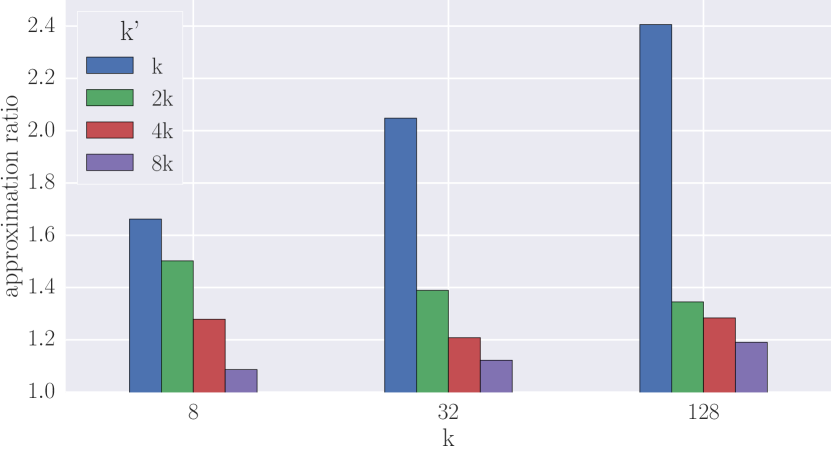
Figure 1: Approximation ratio for the streaming algorithm for different values of $k$ and $k^{\prime}$ on the musiXmatch dataset.

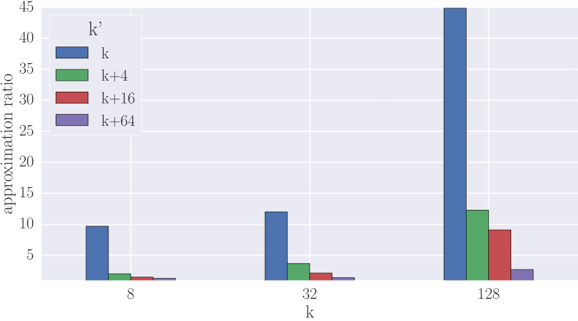
Figure 2: Approximation ratios for the streaming algorithm for different values of $k$ and $k^{\prime}$ on a synthetic dataset of 100 million points.

First, we observe that as $k$ increases the remote-edge measure becomes harder to approximate: finding a higher number of diverse elements is more difficult. On the real-world dataset, because of the high dimensionality of its space, we test the influence of $k^{\prime}$ on the approximation with a geometric progression of $k^{\prime}$ (Figure 2). On the synthetic datasets instead (Figure 2), since $\mathbb{R}^{3}$ has a smaller doubling dimension, the effect of $k^{\prime}$ is evident already with small values, therefore we use a linear progression. As expected, by increasing $k^{\prime}$ the accuracy of the algorithm increases in both datasets. Observe that although the theory suggests that good approximations require rather large values of $k^{\prime}=\Omega(k/\varepsilon^{D})$, in practice our experiments show that relatively small values of $k^{\prime}$, not much larger than $k$, already yield very good approximations, even for the real-world dataset whose doubling dimension is unknown.

In Figure 4, we consider the performance of the kernel of streaming algorithm, that is, we concentrate on the time taken by the algorithm to process each point, ignoring the cost of streaming data from memory. The rationale is that data may be streamed from sources with very different throughput: our goal is to show the maximum rate that can be sustained by our algorithm independently of the source of the stream. We report results for the same combination of parameters shown in Figure 2. As expected, the throughput is inversely proportional to both $k$ and $k^{\prime}$, with values ranging from 3,078 to 544,920 points/s. The throughput supported by our algorithm makes it amenable to be used in streaming pipelines: for instance, in 2013 Twitter averaged at 5,700 tweets/s and peaked at 143,199 tweets/s. In this scenario, it is likely that the bottleneck of the pipeline would be the data acquisition rather than our core-set construction.

As for the synthetic dataset, the throughput of the algorithm exhibits a behavior with respect to $k$ and $k^{\prime}$ similar to the one reported in Figure 4, but with higher values ranging from 78,260 to 850,615 points/s since the distance function is cheaper to compute.

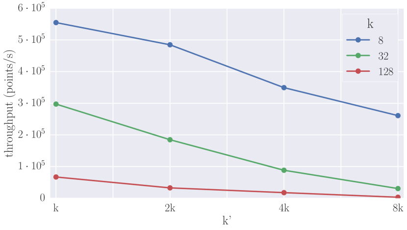
Figure 3: Throughput of the kernel of the streaming algorithm on the musiXmatch dataset.

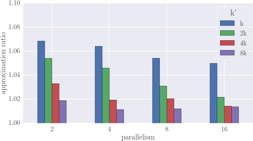
Figure 4: Approximation ratios for the MR algorithm for different values of $k$ and $k^{\prime}$ on a synthetic dataset of 100 million points.

7.2 MapReduce algorithm

We demonstrate our MapReduce algorithm on the same datasets used in the previous section. For this set of experiments we fixed $k=128$ and we varied two parameters: size of the core-sets, as controlled by $k^{\prime}$, and parallelism (i.e., the number of reducers). Because the solution returned by the MapReduce algorithm for $k^{\prime}=k$ turns out to be already very good, we use a geometric progression for $k^{\prime}$ to highlight the dependency of the approximation factor on $k^{\prime}$. The results are reported in Figure 4. For a fixed level of parallelism, we observe that the approximation ratio decreases as $k^{\prime}$ increases, in accordance to the theory. Moreover, we observe that the approximation ratios are in general better than the ones attained by the streaming algorithm, plausibly because in MapReduce we use a 2-approximation $k^{\prime}$-center algorithm to build the core-sets, while in Streaming only a weaker 8-approximation $k^{\prime}$-center algorithm is available.

Figure 4 also reveals that if we fix $k^{\prime}$ and increase the level of parallelism, the approximation ratio tends to decrease. Indeed, the final core-set obtained by aggregating the ones produced by the individual reducers grows larger as the parallelism increases, thus containing more information on the input set. Instead, if we fix the product of $k^{\prime}$ and the level of parallelism, hence the size of the aggregate core-set, we observe that increasing the parallelism is mildly detrimental to the approximation quality. This is to be expected, since with a fixed space budget in the second round, in the first round each reducer is forced to build a smaller and less accurate core-set as the parallelism increases.

The experiments for the real-world musiXmatch dataset (figures omitted for brevity) highlight that the GMM $k^{\prime}$-center algorithm returns very good core-sets on this high dimensional dataset, yielding approximation ratios very close to 1 even for low values of $k^{\prime}$. As remarked above, the more pronounced dependence on $k^{\prime}$ in the streaming case may be the result of the weaker approximation guarantees of its core-set construction.

Since in real scenarios the input might not be distributed randomly among the reducers, we also experimented with an “adversarial” partitioning of the input: each reducer was given points coming from a region of small volume, so to obfuscate a global view of the pointset. With such adversarial partitioning, the approximation ratios worsen by up to $10\%$. On the other hand, as $k^{\prime}$ increases, the time required by a random shuffle of the points among the reducers becomes negligible with respect to the overall running time. Thus, randomly shuffling the points at the beginning may prove cost-effective if larger values of $k^{\prime}$ are affordable.

7.3 Comparison with state of the art

In Table 4, we compare our MapReduce algorithm (dubbed CPPU) against its state of the art competitor presented in [4] (dubbed AFZ). Since no code was available for AFZ, we implemented it in MapReduce with the same optimizations used for CPPU. We remark that AFZ employs different core-set constructions for the various diversity measures, whereas our algorithm uses the same construction for all diversity measures. In particular, for remote-edge, AFZ is equivalent to CPPU with $k^{\prime}=k$, hence the comparison is less interesting and can be derived from the behavior of CPPU itself. Instead, for remote-clique, the core-set construction used by AFZ is based on local search and may exhibit highly superlinear complexity. For remote-clique, we performed the comparison with various values of $k$, on datasets of 4 million points on the 2-dimensional Euclidean space, using 16 reducers (AFZ was prohibitively slow for higher dimensions and bigger datasets). The datasets were generated as described in the introduction to the experimental section. Also, we ran CPPU with $k^{\prime}=128$ in all cases, so to ensure a good approximation ratio at the expense of a slight increase of the running time. As Table 4 shows, CPPU is in all cases at least three orders of magnitude faster than AFZ, while achieving a better quality at the same time.

	approximation		time (s)
k	AFZ	CPPU	AFZ	CPPU
4	1.023	1.012	807.79	1.19
6	1.052	1.018	1,052.39	1.29
8	1.029	1.028	4,625.46	1.12

Table 4: Approximation ratios and running times of our MR algorithm (CPPU) and AFZ.

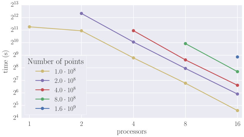
Figure 5: Scalability of our algorithms for different number of points and processors. The running time for one processor is obtained with the streaming algorithm.

7.4 Scalability

We report on the scalability of our MR algorithm on datasets drawn from $\mathbb{R}^{3}$, ranging from 100 million points (the same dataset used in subsections 7.1 and 7.2) up to 1.6 billion points. We fixed the size $s$ of the memory required by the final reducer and varied the number of processors used. On a single machine, instead of running MapReduce, which makes little sense, we run the streaming algorithm with $k^{\prime}=2048$, so to have a final coreset of the same size as the ones found in MapReduce runs. For a given number of processors $p$ and number of points $n$, we run the corresponding experiment only if $n/p$ points fit into the main memory of a single processor. As shown in Figure 5, for a fixed dataset size, our MapReduce algorithm exhibits super-linear scalability: doubling the number of processors results in a 4-fold gain in running time (at the expense of a mild worsening of the approximation ratio, as pointed out in Subsection 7.2). The reason is that each reducer performs $O\left(ns/(kp^{2})\right)$ work to build its core-set, where $p$ is the number of reducers, since the core-set construction involves $s/(kp)$ iterations, with each iteration requiring the scan of $n/p$ points.

For the dataset with 100 million points, the MR algorithm outperforms the streaming algorithm in every processor configuration. It must be remarked that the running time reported in Figure 5 for the streaming algorithm takes into account also the time needed to stream data from main memory (unlike the throughput reported in Figure 4). This is to ensure a fair comparison with MapReduce, where we also take into account the time needed to shuffle data between the first and the second round, and the setup time of the rounds. Also, we note that the streaming algorithm appears to be faster than what the MR algorithm would be if executed on a single processor, and this is probably due to the fact that the former is more cache friendly.

If we fix the number of processors, we observe that our algorithm exhibits linear scalability in the number of points. Finally, in a set of experiments, omitted for brevity, we verified that for a fixed number of processors the time increases linearly with $k^{\prime}$. Both these behaviors are in accordance with the theory.

8 Acknowledgments

Part of this work was done while the authors were visiting the Departiment of Computer Science at Brown University. This work was supported, in part, by MIUR of Italy under project AMANDA, and by the University of Padova under project CPDA152255/15: ”Resource-Tradeoffs Based Design of Hardware and Software for Emerging Computing Platforms”. The work of Eli Upfal was supported in part by NSF grant IIS-1247581 and NIH grant R01-CA180776.

References

- [1] Z. Abbassi, V. S. Mirrokni, and M. Thakur. Diversity maximization under matroid constraints. In Proc. ACM KDD, pages 32–40, 2013.
- [2] M. Ackermann, J. Blömer, and C. Sohler. Clustering for metric and nonmetric distance measures. ACM Trans. on Algorithms, 6(4):59, 2010.
- [3] P. Agarwal, S. Har-Peled, and K. Varadarajan. Geometric approximation via coresets. Combinatorial and computational geometry, 52:1–30, 2005.
- [4] S. Aghamolaei, M. Farhadi, and H. Zarrabi-Zadeh. Diversity maximization via composable coresets. In Proc. CCCG, pages 38–48, 2015.
- [5] A. Angel and N. Koudas. Efficient diversity-aware search. In Proc. SIGMOD, pages 781–792, 2011.
- [6] T. Bertin-Mahieux, D. P. Ellis, B. Whitman, and P. Lamere. The million song dataset. In Proc. ISMIR, 2011.
- [7] S. Bhattacharya, S. Gollapudi, and K. Munagala. Consideration set generation in commerce search. In Proc. WWW, pages 317–326, 2011.
- [8] M. Ceccarello, A. Pietracaprina, G. Pucci, and E. Upfal. Space and time efficient parallel graph decomposition, clustering, and diameter approximation. In Proc. ACM SPAA, pages 182–191, 2015.
- [9] M. Ceccarello, A. Pietracaprina, G. Pucci, and E. Upfal. A practical parallel algorithm for diameter approximation of massive weighted graphs. In Proc. IEEE IPDPS, 2016.
- [10] M. Ceccarello, A. Pietracaprina, G. Pucci, and E. Upfal. Mapreduce and streaming algorithms for diversity maximization in metric spaces of bounded doubling dimension. PVLDB, 10(5):469–480, 2017.
- [11] A. Cevallos, F. Eisenbrand, and R. Zenklusen. Max-sum diversity via convex programming. In Proc. SoCG, volume 51, page 26, 2016.
- [12] B. Chandra and M. Halldórsson. Approximation algorithms for dispersion problems. J. of Algorithms, 38(2):438–465, 2001.
- [13] M. Charikar, C. Chekuri, T. Feder, and R. Motwani. Incremental clustering and dynamic information retrieval. SIAM J. on Computing, 33(6):1417–1440, 2004.
- [14] Z. Chen and T. Li. Addressing diverse user preferences in SQL-query-result navigation. In Proc. SIGMOD, pages 641–652, 2007.
- [15] R. Cole and L. Gottlieb. Searching dynamic point sets in spaces with bounded doubling dimension. In Proc. ACM STOC, pages 574–583, 2006.
- [16] S. Fekete and H. Meijer. Maximum dispersion and geometric maximum weight cliques. Algorithmica, 38(3):501–511, 2004.
- [17] S. Gollapudi and A. Sharma. An axiomatic approach for result diversification. In Proc. WWW, pages 381–390, 2009.
- [18] T. F. Gonzalez. Clustering to minimize the maximum intercluster distance. Theoretical Computer Science, 38:293 – 306, 1985.
- [19] L. Gottlieb, A. Kontorovich, and R. Krauthgamer. Efficient classification for metric data. IEEE Trans. on Information Theory, 60(9):5750–5759, 2014.
- [20] A. Gupta, R. Krauthgamer, and J. R. Lee. Bounded geometries, fractals, and low-distortion embeddings. In Proc. IEEE FOCS, pages 534–543, 2003.
- [21] M. Halldórsson, K. Iwano, N. Katoh, and T. Tokuyama. Finding subsets maximizing minimum structures. SIAM Journal on Discrete Mathematics, 12(3):342–359, 1999.
- [22] R. Hassin, S. Rubinstein, and A. Tamir. Approximation algorithms for maximum dispersion. Operations Research Letters, 21(3):133 – 137, 1997.
- [23] P. Indyk, S. Mahabadi, M. Mahdian, and V. Mirrokni. Composable core-sets for diversity and coverage maximization. In Proc. ACM PODS, pages 100–108, 2014.
- [24] H. Karloff, S. Suri, and S. Vassilvitskii. A model of computation for MapReduce. In Proc. ACM-SIAM SODA, pages 938–948, 2010.
- [25] G. Konjevod, A. Richa, and D. Xia. Dynamic routing and location services in metrics of low doubling dimension. In Distributed Computing, pages 379–393. Springer, 2008.
- [26] J. Leskovec, A. Rajaraman, and J. Ullman. Mining of Massive Datasets, 2nd Ed. Cambridge University Press, 2014.
- [27] M. Masin and Y. Bukchin. Diversity maximization approach for multiobjective optimization. Operations Research, 56(2):411–424, 2008.
- [28] S. Munson, D. Zhou, and P. Resnick. Sidelines: An algorithm for increasing diversity in news and opinion aggregators. In Proc. ICWSM, 2009.
- [29] A. Pietracaprina, G. Pucci, M. Riondato, F. Silvestri, and E. Upfal. Space-round tradeoffs for MapReduce computations. In Proc. ACM ICS, pages 235–244, 2012.
- [30] P. Raghavan and M. Henzinger. Computing on data streams. In Proc. DIMACS Workshop External Memory and Visualization, volume 50, page 107, 1999.
- [31] D. Rosenkrantz, S. Ravi, and G. Tayi. Approximation algorithms for facility dispersion. In Handbook of Approximation Algorithms and Metaheuristics. 2007.
- [32] A. Tamir. Obnoxious facility location on graphs. SIAM J. on Discrete Mathematics, 4(4):550–567, 1991.
- [33] Y. Wu. Active learning based on diversity maximization. Applied Mechanics and Materials, 347(10):2548–2552, 2013.
- [34] Y. Yang, Z. Ma, F. Nie, X. Chang, and A. Hauptmann. Multi-class active learning by uncertainty sampling with diversity maximization. Int. J. of Computer Vision, 113(2):113–127, 2015.
- [35] C. Yu, L. Lakshmanan, and S. Amer-Yahia. Recommendation diversification using explanations. In Proc. ICDE, pages 1299–1302, 2009.