EFTfitter—A tool for interpreting measurements in the context of effective field theories

Abstract

Over the past years, the interpretation of measurements in the context of effective field theories has attracted much attention in the field of particle physics. We present a tool for interpreting sets of measurements in such models using a Bayesian ansatz by calculating the posterior probabilities of the corresponding free parameters numerically. An example is given, in which top-quark measurements are used to constrain anomalous couplings at the $Wtb$-vertex.

1 Introduction

With the recent start of the Run-2 of the LHC, searches for physics beyond the Standard Model (BSM) will reach unprecedented sensitivity. The LHC’s increased centre-of-mass energy opens a new kinematic regime and enhances the direct production cross section of heavy, yet unknown, particles—if they exist. It is a good time for bump hunters.

On the other hand, it is not obvious that the mass scale of such new particles is anywhere near the energy which can be reached by current, or even future, accelerators. However, in contrast to the direct production of heavy particles, their impact on observables accessible at current collider experiments can be probed indirectly in the context of effective field theories. Such theories extend the Standard Model (SM) Lagrangian by terms allowed in quantum field theory and which share the gauge symmetries of the SM. These terms contain one or several effective operators and corresponding coefficients, often referred to as Wilson coefficients, which define the individual strength of these operators. Depending on the type of operator, the additional terms in the Lagrangian can have an impact on different observables, which, in turn, can be compared to a set of corresponding measurements. Comparisons of SM predictions and observations can be used to constrain the Wilson coefficients by propagation of uncertainty. The strategy to indirectly infer on the parameters of a physics model, may it be an effective model or a full model, has proven to be successful in a variety of applications, e.g. in the field of flavor physics Beaujean:2013soa , super-symmetry Bechtle:2004pc , or electroweak precision measurements Flacher:2008zq .

This paper describes a generic tool, the EFTfitter, for performing such interpretations in the context of user-defined physics models and formulating them in terms of Bayesian reasoning. Emphasis is placed on the statistical treatment of the combination of measurements correlated by their uncertainties as well as on often overlooked issues in interpretations, such as the necessity to consider model-specific efficiency and acceptance corrections for the measurements, or the presence of physical constraints on observables and parameters. An example is given for the case of an effective field theory in the top-quark sector, which is an active field of research. This example is motivated by the wealth of experimental data delivered by the Tevatron and LHC experiments and the increasing precision of measurements involving top quarks. Also from a theoretical perspective, the interpretation of top-quark measurements is attractive: recent calculations, e.g. predictions of the cross section of top-quark pair production Czakon:2012pz ; Czakon:2011xx ; Czakon:2013goa , reach next-to-next-to-leading order (NNLO) precision in perturbative QCD. A historical example for the interpretation of experimental data in the context of top quarks is the successful prediction of the top-quark mass from electroweak precision measurements, see, e.g., Ref. Langacker:1991an .

This paper is organised as follows. Section 2 describes the statistical procedure of combining several measurements, while their interpretation is discussed in Section 3. The numerical implementation of the EFTfitter is introduced in Section 4, and an example for interpretations in the field of top-quark physics is given in Section 5. The paper is concluded in Section 6.

2 Combination of measurements

In Bayesian reasoning, inference of the free parameters $\vec{\lambda}$ of a model $M$ is based on the posterior probability of those parameters given a data set $\vec{x}$, $p(\vec{\lambda}|\vec{x})$. It is calculated using the equation of Bayes and Laplace Bayes:1764vd ,

$$p(\vec{\lambda}|\vec{x})=\frac{p(\vec{x}|\vec{\lambda})\cdot p(\vec{\lambda})}{p(\vec{x})}\,,$$ (1)

where $p(\vec{x}|\vec{\lambda})$ is the probability of the data, or likelihood, and $p(\vec{\lambda})$ is the prior probability of the parameters $\vec{\lambda}$. In Bayesian literature, the normalisation constant in the denominator,

$$p(\vec{x})=\int{\mathrm{d}\vec{\lambda}\,}\,p(\vec{x}|\vec{\lambda})\cdot p(\vec{\lambda})\,,$$ (2)

is often referred to as the evidence.

In the following, we distinguish two types of models: i) those for which the parameters can be directly measured from the data, and ii) those for which this is not the case. Models of type ii) typically predict values of physical quantities, or observables, $\vec{y}$, which depend on the parameters of the model, $\vec{\lambda}$, so that $\vec{y}=\vec{y}(\vec{\lambda})$. For example, the predicted cross sections in scattering processes depend on the couplings and masses of the particles described by physics models. These couplings and masses are often not predicted by the models themselves, in which case they are free parameters. Couplings, e.g., can often only be estimated indirectly from the measurements of cross sections and other observables. This case will be discussed further in Section 3. On the other hand, models of type i) are often used for the plain combination of measurements in which the physical quantities themselves, e.g. cross sections, angular distributions or branching ratios, are interpreted as model parameters, i.e., $\vec{y}=\vec{\lambda}$. We will discuss this case in the following.

2.1 Combination of measurements

Following the notation of Ref. Valassi:2003mu , we assume to have $N$ observables, $y_{i}~{}(i=1,\dots,N)$, which are estimated based on $n$ measurements, $x_{i}~{}(i=1,\dots,n)$. Each quantity $y_{i}$ is measured $n_{i}\geq 1$ times, so that $n=\sum_{i=1}^{N}n_{i}\geq N$. We adopt the common assumption that the likelihood terms in Eqn. (1), $p(\vec{x}|\vec{y})$, have a multivariate Gaussian shape, and that the uncertainties of the measurements of $x_{i}$ can be correlated. The elements of the symmetric and positive-semidefinite covariance matrix are

$$\mathcal{M}_{ij}=\mathrm{cov}[x_{i},x_{j}]\,.$$ (3)

Assuming $M$ different sources of uncertainty, the covariance matrix can be decomposed into contributions from each source,

$$\mathrm{cov}[x_{i},x_{j}]=\sum_{k=1}^{M}\mathrm{cov}^{(k)}[x_{i},x_{j}]\,.$$ (4)

The likelihood can then be expressed as

$$-2\ln p(\vec{x}|\vec{y})=\sum_{i=1}^{n}\sum_{j=1}^{n}\left[\vec{x}-U\vec{y}\right]_{i}\mathcal{M}_{ij}^{-1}\left[\vec{x}-U\vec{y}\right]_{j}\,,$$ (5)

where the elements $U_{ij}$ of the $n\times N$-matrix $U$ are unity if $x_{i}$ is a measurement of the observable $y_{j}$, and zero otherwise.

The best linear unbiased estimator (BLUE) Valassi:2003mu ; Lyons:1988rp can be found by minimising the expression in Eqn. (5), while an estimator in the Bayesian approach is constructed by inserting Eqn. (5) into the RHS of Eqn. (1), and by specifying prior probabilities for the parameters. The prior probabilities can include physical constraints, e.g. the requirements that cross-sections can only take positive values or that branching ratios lie between zero and one. Prior knowledge can also come from auxiliary measurements or theoretical considerations. It is worth noting that combined estimates of physical quantities based on individual posterior probabilities need to be cleaned from the corresponding prior probabilities, i.e. the prior information about a parameter should only be included once in the overall combination. It should also be noted that prior probabilities, and in particular physical constraints, can lead to a strong non-Gaussian shape of the resulting posterior probability distribution, even if the input measurements are assumed to be described by Gaussian probability densities.

Typical estimators are the set of parameters which maximise the posterior probability, the mean values of the posterior probability distribution, or the set of parameters which maximise the marginal probabilities,

$$p(y_{i}|\vec{x})=\int\prod_{j\neq i}{\mathrm{d}y_{j}\,}\,p(\vec{y}|\vec{x})\,.$$ (6)

For uniform prior probabilities, and in the absence of further constraints, the global mode of the posterior corresponds to the BLUE solution Lyons:1988rp . The uncertainty on $y_{i}$ can be defined as the central interval containing 68% probability, the set of smallest intervals containing 68% probability or simply the standard deviation of the marginalised posterior. These three measures are equal for Gaussian distributions. Similarly, simultaneous estimates of the uncertainties on $y_{i}$ and $y_{j}$ can be obtained by the two-dimensional contours of the smallest intervals containing, e.g., 39% or 68% probability.  Upper and lower limits on $y_{i}$ are typically set by calculating the 90% or 95% quantiles of the corresponding marginal posterior distribution.

2.2 Uncertainties of the correlation

Although it is often straightforward to obtain estimates of the quantities $\vec{y}$ and of their uncertainties, it is not trivial to quantify the correlation induced by the different sources of uncertainties. If, e.g., sources of systematic uncertainty have an impact on several of those measurements, the correlation is often assumed to be extreme ($\rho=\pm 1$). On the other hand, correlated statistical uncertainties caused by partially overlapping data sets are often estimated using pseudo data: two measurements, $x_{i}$ and $x_{j}$, are obtained from common sets of simulated data and the linear correlation coefficient $\rho_{ij}=\mathrm{cov}[x_{i},x_{j}]/\sigma_{i}\sigma_{j}$ between the estimates is calculated. Here, $\sigma_{i}$ and $\sigma_{j}$ are the standard deviations of $x_{i}$ and $x_{j}$, respectively.

If no reliable estimate of the correlation is possible, one can associate correlation coefficients with nuisance parameters $\vec{\nu}$ and choose suitable prior probabilities for these parameters. Necessary requirements for the priors are that the correlation coefficients are constrained to be in the interval $[-1,+1]$, and that the covariance matrix remains positive-semidefinite for all possible values of $\vec{\nu}$. They should, however, parameterise the prior knowledge about the correlation, e.g. by restricting the correlation coefficients to be positive or by favouring mild correlations. Depending on the problem, it can be difficult to formulate such priors analytically. In particular, it is advisable to not allow values resulting in correlation coefficients of $\rho=\pm 1$ for the entries of the total covariance matrix as those might lead to numerical instabilities. Prior probabilities for covariance matrices are proposed in the literature, see e.g. Refs. Leonard1992 ; Barnard2000 ; Huag2013 . The covariance matrix $\mathcal{M}$, and thus the likelihood, are then functions of $\vec{\nu}$, so that $p(\vec{x}|\vec{y},\,\vec{\nu})$. The prior probability can be factorised, $p(\vec{y},\,\vec{\nu})=p(\vec{y})\cdot p(\vec{\nu})$, if $\vec{y}$ and $\vec{\nu}$ are assumed to be independent, which is typically the case. In order to obtain a function depending only on $\vec{y}$ alone, all nuisance parameters are integrated out,

$$p(\vec{y}|\vec{x})=\int{\mathrm{d}\vec{\nu}\,}\,p(\vec{y},\,\vec{\nu}|\vec{x})\,,$$ (7)

and the estimates of $\vec{y}$ are obtained as before from the resulting marginal posterior probabilities.

2.3 Propagation of uncertainty

In cases where the probability density for a quantity $f(\vec{y})$ is needed, the uncertainty on $\vec{y}$ needs to be propagated to $f$. For Gaussian posterior probabilities, the propagation of uncertainty is often done using the well-known rules for uncertainty propagation. These imply that the function $f$ can be linearised in $\vec{y}$ and that the posterior probability for the quantity of interest also has a Gaussian shape. Since this is not always the case, and since the posterior of the combination does not have to be a Gaussian due to the additional prior information, we instead propose to use a numerical evaluation of the uncertainty: if it is possible to sample from the posterior distribution $p(\vec{y}|\vec{x})$, one can calculate the target quantity $f(\vec{y})$ for each sampled point. The obtained frequency distribution for $f$ converges to the posterior probability distribution $p(f|\vec{x})$ in the large sample limit. As discussed in Section 4, such sampling can be done on-the-fly when using Markov Chain Monte Carlo (MCMC).

2.4 Ranking the impact of individual measurements

One is often interested in how much a single measurement contributes to a combination. In BLUE averages, the contributions are added linearly using weights: the larger the weight, the more important the measurement. Although counter-intuitive at first sight, these weights can also take negative values, induced by strong negative correlations, see e.g. the discussion in Refs. Valassi:2003mu ; Lyons:1988rp .

There are several ways to estimate the impact of individual measurements in a combination. For the approach discussed here, we propose to repeat the combination while removing one measurement from the combination at a time. The measurements can then be ranked according to the resulting increase in uncertainty compared to the uncertainty of the overall combination. For combinations with two ($n$) physical quantities, the area (volume) of the smallest contour (hyper-sphere) covering, e.g., 68.3% of the posterior probability, can be used as a rank indicator. The motivation for this choice is to answer the question how the combination would change if a particular measurement had not been considered in the combination.

Regardless of the choice of rank indicator, the estimators themselves, their uncertainties and the correlations between the physical quantities should be monitored during this procedure. Note that the uncertainty can also decrease if particular measurements are removed, as in the case of outliers.

2.5 Ranking the impact of individual sources of uncertainty

The situation is similar when one aims to rank the sources of uncertainties in order of their importance. We propose to repeat the combination while removing one source of uncertainty from the combination at a time. The sources of uncertainty can then be ranked according to the resulting decrease of uncertainty compared to the uncertainty of the overall combination. The rank indicator can be extended to $n$-dimensional problems. From a practical point of view, this approach allows answering the question which source of uncertainty is most important to improve in future iterations of the measurements.

3 Interpretation of measurements in physics models

Estimating the parameter values $\vec{\lambda}$ of a complex physics model $M$ based on (the combination of) measurements and the subsequent propagation of uncertainties is an inverse problem which is often ill-posed and in most cases difficult to solve. We propose here to re-formulate the problem discussed in the previous section in the following way: instead of directly identifying the observables with the fit parameters, we instead fit the free parameters of the physics model under study based on the relation between the observables and the parameters. If the model predicts observables $y_{i}$ for each set of parameter values $\vec{\lambda}$, $y_{i}=y_{i}(\vec{\lambda})$, these are then compared to the measurements $x_{i}$ using a multivariate Gaussian model. The same formalism as in Section 2.1 can be used to estimate $\vec{\lambda}$ for a given data set. The likelihood of the model is

$$p(\vec{x}|\vec{\lambda})=\int{\mathrm{d}\vec{y}\,}\,p(\vec{x}|\vec{y})\cdot p(\vec{y}|\vec{\lambda})\,,$$

where $p(\vec{y}|\vec{\lambda})=\delta(\vec{y}-\vec{y}(\vec{\lambda}))$. It is worth noting that one has to formulate prior probabilities in terms of the model parameters and not in terms of the measurements themselves. Physical constraints can be incorporated into the model predictions, ‘external knowledge’ can be viewed as an additional measurement. 

Using the same framework also helps to include measurements and physical quantities in the analysis which would otherwise be combined separately, e.g. by a working group concerned with cross sections and another one interested in angular distributions. However, due to common sources of systematic uncertainties and overlapping data sets, the posterior probability of the two measurements shows a correlation—a fact that needs to be considered in the global fit to a physics model.

4 Implementation

The EFTfitter  builds on the Bayesian Analysis Toolkit (BAT) Caldwell:2008fw which is a software package written in C++ that allows the implementation of statistical models and the inference on their free parameters.  Several numerical algorithms can be used to perform the combination and interpretation steps introduced in this paper: marginal distributions can be calculated using, for example, Markov Chain Monte Carlo, while global optimisation can be done using the Minuit implementation of ROOT Brun:1997pa .

4.1 Definition of a model and observables

The key component of the EFTfitter is the user’s definition of a model. It is simply characterised by a set of free parameters, e.g. couplings and masses, and by the predictions of observables as a function of the model’s parameters. Note that the model is not automatically derived from a user-defined Lagrangian and it is thus not constrained to a particular class of models. As a consequence, however, the predictions from the model are not required to be consistent, and it is the user’s responsibility to formulate a meaningful set of predictions. Of course, interfaces to more complex software tools can be included in the model.

4.2 Input

The input to the EFTfitter is a set of measurements including a break-down of the uncertainties into several categories, e.g. statistical uncertainties and different sources of systematic uncertainties. In addition, the correlation between the measurements for each category of uncertainty needs to be provided.

It is worth noting that the different measurements need to be unified in a sense that the sources of uncertainties are treated in the same categories throughout all measurements, e.g. uncertainties related to the reconstruction of objects in a collider experiment should have one or more well-defined categories: uncertainties on the luminosity, efficiencies or acceptances should each have their own categories, etc.

The measurements can be any measurable quantity, most commonly a cross section, a mass or a branching ratio. It can also be an unfolded spectrum, in which case each bin is treated as an individual measurement and the full unfolding matrix is needed as an input. The unfolding matrix provides the acceptances and efficiencies, which can be treated consistently in the EFTfitter as described in Sec. 4.3.

All of these inputs are provided in a configuration file in xml format. The file contains information about the number of observables, the number of measurements of these observables, the number of uncertainty categories and the number of nuisance parameters to be used in the fit. The allowed range for each observable has to be provided. For each measurement, the name of the observable, its measured value as well as its uncertainty in each uncertainty category have to be provided as well. Furthermore, measurements can be omitted from the fit by flagging them as inactive. The correlation matrix is provided in the same configuration file. The correlation coefficients between measurements can be treated as nuisance parameters in the fit. For each nuisance parameter, the measurements that the correlation coefficient refers to as well as its prior probability have to be specified.

Apart from the measurements, the user needs to specify prior probability densities for each model parameter. These can be chosen freely, e.g. uniform, Gaussian or exponentially decreasing functions. Physical boundaries for parameters and observables are addressed by the definition of the prior probabilities and the predictions for observables, respectively. A second configuration file in xml format is used to specify the prior probability densities for the parameters, their minimum and maximum values, as well as their SM predictions.

Sometimes it is necessary to include external input in a combination, e.g. measurements from low-energy observables, $b$-physics or cosmology. These can either be treated as additional measurements or as priors on the parameters, depending on the type of information provided. In both cases, it is usually difficult to estimate the correlation between the different inputs and the user should carefully consider whether the choice of correlation made has a strong effect on the interpretation of the data.

4.3 Treatment of acceptance and efficiency corrections

A problem often encountered when measurements are interpreted in terms of BSM contributions, is that the acceptances and efficiencies may be different for different BSM processes, while measurements are mostly performed assuming the acceptances and efficiencies of SM processes. An example is the measurement of the cross section for the pair production of a particle, which in BSM scenarios might also be produced from an additional resonance decay. The acceptance times efficiency for the BSM process may be different than for the SM process if the measurement requires a minimum momentum for the final-state particles. These requirements may be more frequently fulfilled in the BSM scenario if the resonance has a very high mass. It is also clear that the acceptance and efficiency may depend on the parameters of the BSM theory, such as the mass of the resonance in this example.

The EFTfitter addresses this problem by separating observables, measurements and parameters, so that the acceptance and efficiency can be corrected for when comparing the prediction for the observables with the measurements. For the SM process, this acceptance and efficiency correction is equal to unity, but for BSM models, the correction may differ from one and it is, in general, a function of the parameters of the theory.

4.4 Output

A brief summary of the fit results is provided in a text file, while four figure files are provided for a more detailed analysis of the fit results. In one figure file, all one-dimensional and two-dimensional marginalised distributions of the fitted parameters are saved. In two figure files, the estimated correlation matrix of the parameters and a comparison of the prior and posterior probability density functions for the different parameters are shown, respectively. A last figure file shows the relations between the parameters of the model and the observables as defined by the underlying model. An additional text file provides the post-fit ranking of the measurements determined as described in Sections 2.4 and 2.5.

4.5 Structure of the implementation

The code is structured such that a new folder needs to be created for a specific analysis. Folders are provided for the example discussed in this paper (Sec. 5) as well as a blank example a user can start from. Each such folder contains a subfolder for the input configuration files and an empty folder for the result files. It also contains a rather generic run file which holds the main function for the run executable. The model specific details, such as the relation between the parameters and the observables, the acceptance and efficiency correction etc. are implemented in a class inheriting from BCMVCPhysicsModel. In this class, it is necessary to provide in particular a concrete implementation of the virtual method CalculateObservable(…). The code is then compiled using a Makefile, which is provided. A README file contains further details for users to get started.

5 An example for effective field theory involving top quarks

As an example for applications of the EFTfitter, we discuss the constraints on anomalous top-quark couplings from two sets of observables: the measurement of the polarisation of $W$-bosons produced in top-quark decays and the measurements of the $t$-channel top- and antitop-quark cross sections. Similar cases have been discussed in Refs. AguilarSaavedra:2006fy ; AguilarSaavedra:2008gt ; AguilarSaavedra:2008zc ; Zhang:2010dr ; Buckley:2015nca ; Buckley:2015lku ; Bernardo:2014vha ; Fabbrichesi:2014wva ; Birman:2016jhg . The concrete model we use is that of Ref. AguilarSaavedra:2006fy , where the Lagrangian describing the $Wtb$-vertex does not only include a purely left-handed coupling with relative strength $V_{L}$, but also a right-handed vector coupling with strength $V_{R}$ as well as left- and right-handed tensor couplings $g_{L}$ and $g_{R}$. The generalised Lagrangian then takes the form

$$\mathcal{L} = -\frac{g}{\sqrt{2}}\bar{b}\gamma^{\mu}\left(V_{L}P_{L}+V_{R}P_{R}\right)tW_{\mu}^{-}-$$ (9)

$$\frac{g}{\sqrt{2}}\bar{b}\frac{i\sigma^{\mu\nu}q_{\nu}}{M_{W}}\left(g_{L}P_{L}+g_{R}P_{R}\right)tW_{\mu}^{-}+h.c.\,,$$

where $g$ is the weak coupling constant, $P_{L}$ and $P_{R}$ are left- and right-handed projection operators and $M_{W}$ is the mass of the $W$-boson. In the SM, the left-handed coupling strength is given by $V_{L}=\left|V_{tb}\right|^{2}\approx 1$, while the three other coupling strengths are $V_{R}=g_{L}=g_{R}=0$.

The physical model defined by the Lagrangian in Eqn. (9) has four free parameters: $V_{L}$, $V_{R}$, $g_{L}$, $g_{R}$. For simplicity, we assume these parameters to be real.

5.1 Observables and predictions

The observables described in the following are calculated based on Refs. AguilarSaavedra:2006fy ; AguilarSaavedra:2008gt ; Bach:2014zca . The masses of the top quark, the $W$-boson and the bottom quark are assumed to be $172.5\,\mathrm{GeV}$, $80.4\,\mathrm{GeV}$ and $4.8\,\mathrm{GeV}$, respectively.

The $W$-bosons produced in top-quark decays can be left-handed, right-handed and longitudinally polarised. The fraction of events with either of these polarisations are $f_{L}$, $f_{R}$ and $f_{0}$, and often referred to as helicity fractions. At NNLO accuracy in the strong coupling, these fractions are predicted to be $f_{L}=0.311\pm 0.005$, $f_{R}=0.0017\pm 0.0001$ and $f_{0}=0.687\pm 0.005$ in the SM Czarnecki:2010gb . Assuming the Lagrangian defined in Eqn. (9), these fractions are functions of the four coupling strengths. As an example, Fig. 1 shows the predicted fraction of left-handed $W$-bosons as a function of any of the couplings in the range $[-1,+1]$, while keeping the other three couplings fixed to their SM values. While the variation of $V_{R}$ and $g_{L}$ results in variations of $f_{L}$ from about 15% to a maximum of roughly 30% at $V_{R}=0$ and $g_{L}=0$, $g_{R}$ has a stronger impact. The value of $f_{L}$ ranges from 0% to about 70% with a minimum at approximately $g_{R}=0.5$. As expected, there is no dependence of the helicity fractions on $V_{L}$. Since the sum of the three fractions is unity, only two of the three, $f_{L}$ and $f_{0}$, are considered as well as their correlation.

Similarly, the cross sections for single top- and antitop-quark production in the $t$-channel at a centre-of-mass-energy of $\sqrt{s}=7\,\mathrm{TeV}$ are predicted in the SM to be $\sigma_{t}=41.9^{+1.8}_{-0.8}\,\mathrm{pb}$ and $\sigma_{\bar{t}}=22.7^{+0.9}_{-1.0}\,\mathrm{pb}$ at NNLO accuracy in the strong coupling Kidonakis:2011wy . As an example, the single top-quark cross section as a function of the four coupling strengths is illustrated in Fig. 2, again fixing the other couplings to their SM values for each of the curves. All four couplings change the predicted cross section resulting in values of $\sigma_{t}$ between 0 $\mathrm{pb}$ and 140 $\mathrm{pb}$, where a minimum can be found at coupling values of about 0.

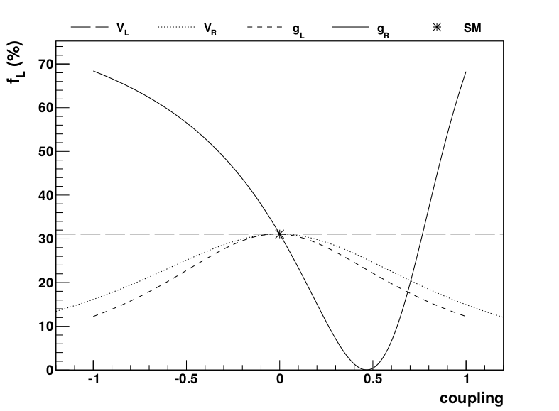
Figure 1: Fraction of left-handed $W$-bosons from top-quark decays as a function of anomalous couplings. The asterisk indicates the SM values.

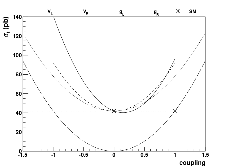
Figure 2: Cross section for $t$-channel single top-quark production as a function of anomalous couplings. The asterisk indicates the SM values.

5.2 Measurements and assumptions

The measurements of the $W$-boson polarisation and the $t$-channel cross sections considered in this example are taken from Refs. Chatrchyan:2013jna and Aad:2014fwa , respectively. The uncertainties on these measurements are assumed to be derived from multivariate Gaussian distributions. The measured values are

$$f_{L} = 0.310\pm 0.031$$

$$f_{0} = 0.682\pm 0.045$$

$$\sigma_{t} = 46\pm 6\,\mathrm{pb}$$

$$\sigma_{\bar{t}} = 23\pm 3\,\mathrm{pb}\,.$$

The correlation between the measurements of $f_{L}$ and $f_{0}$ is quoted in the reference as $\rho(f_{L},f_{0})=-0.95$. We assume that there is no correlation between the helicity and cross-section measurements. This simplifying assumption is made because the measurements are performed by two different experiments and because the event selections for the two measurements are orthogonal. Common sources of systematic uncertainty, e.g. from LHC machine settings or the modelling of top quarks in Monte Carlo generators, could lead to a small correlation, however. Furthermore, we assume that the correlation between the measurements of top- and antitop-quark cross sections is mild, but not negligible, and we thus choose $\rho(\sigma_{t},\sigma_{\bar{t}})=+0.50$. Although the event selections are again orthogonal—the leptons selected differ by the sign of their electric charge—common sources of systematic uncertainty have a similar impact on both measurement, e.g. uncertainties on the jet-energy and lepton-momentum scales or the Monte Carlo generator uncertainties. The total uncertainties and the full correlation matrix used are shown in Tab. 1.

Table 1: Total uncertainties and the correlation matrix of the helicity fraction and $t$-channel cross section measurements.

	Uncertainty	$f_{L}$	$f_{0}$	$\sigma_{t}$	$\sigma_{\bar{t}}$
$f_{L}$	0.031	1.00	-0.95	0.00	0.00
$f_{0}$	0.045	-0.95	1.00	0.00	0.00
$\sigma_{t}$	6 pb	0.00	0.00	1.00	0.50
$\sigma_{\bar{t}}$	3 $\mathrm{pb}$	0.00	0.00	0.50	1.00

The efficiency times acceptance of the measured $t$-channel cross section depends on the anomalous couplings assumed because they have an impact on the kinematic distributions of the final-state particles. Since its evaluation would require further studies including simulations of the detector setup and a repetition of the analysis procedure, they are not considered in this example. In general, these corrections should be provided by the experimental collaborations as such an evaluation often requires access to unpublished material. As described in Section 4.3, the EFTfitter code is prepared to include such correlations.

5.3 Interpretation of measurements

We assume no prior knowledge on the values of the four coupling strengths, i.e. we choose the prior probability density for each coupling to be uniform. The values of $g_{L}$ and $g_{R}$ are limited to a range $[-1,1]$, the values of $V_{L}$ and $V_{R}$ are constrained to be within $[-1.5,1.5]$. These ranges are motivated by the fact that larger anomalous couplings would have been observed by previous measurements.

For the first interpretation, we assume SM values for the vector couplings, i.e., we assume $V_{L}=1$ and $V_{R}=0$. Taking all four measurements and their correlations into account, Figure 3 shows the contours of the smallest areas containing 68.3% and 95.5% probability in the two-dimensional plane of $g_{R}$ vs. $g_{L}$. In comparison, the dark and coloured lines indicate these contours if only the measurements of the $W$-helicity or of the $t$-channel cross sections are considered. While the measurement of the $W$-helicity alone constrains two separate regions in $(g_{L},g_{R})$-space, one centred around the SM prediction of $(0,0)$ and another, smaller one around $(0,0.8)$, the measurement of the $t$-channel cross sections has less constraining power, but excludes the second region. Using all four measurements thus reduces the available parameter space for anomalous couplings by excluding the second region and, if only marginally, by reducing the area of the first region.

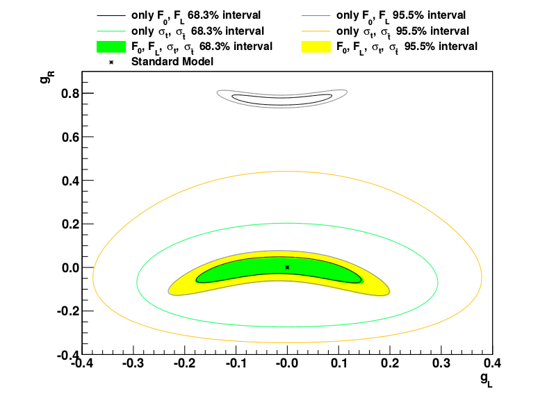
Figure 3: Contours of the smallest areas containing 68.3%, 95.5% and 99.7% posterior probability in the $(g_{L},g_{R})$-plane. The filled areas consider all four measurements, while the open ones take into account only two measurements. Also indicated is the SM prediction.

The relative importance of each of the four measurements is illustrated in Tab. 2, which shows a ranking based on the relative increase of the area within the 68.3% contour if individual measurements are ignored. This is compared to a ranking based on the uncertainties of the one-dimensional marginal distributions. As expected from Fig. 3, the measurements of the $W$-helicity have a larger impact on the constraints than the $t$-channel measurements. It is worth noting, however, that the ranking only addresses the size of the uncertainties, but not the topology of the contours, i.e. the appearance of a second, disconnected allowed region. The small negative values associated with the measurement of $\sigma_{t}$ can be explained by the fact that the measured value is furthest away from the SM prediction in comparison to the other three measurements.

Table 2: Relative increase of the area contained in the 68.3% posterior probability contour when removing one measurement at a time. Also indicated is the rank.

Measurement	Relative increase [%] (rank)
	$(g_{L},g_{R})$	$g_{L}$	$g_{R}$
$f_{0}$	162.3 (2.)	83.7 (1.)	17.6 (2.)
$f_{L}$	281.5 (1.)	66.3 (2.)	88.2 (1.)
$\sigma_{\bar{t}}$	-002.2 (3.)	2.2 (3.)	0.0 (3.)
$\sigma_{t}$	-003.2 (4.)	-05.4 (4.)	-02.9 (4.)

As an example, we test the impact of the correlation between $\sigma_{t}$ and $\sigma_{\bar{t}}$ on the estimate of $g_{R}$. Fig. 4 shows the one-dimensional marginal posterior probability for $g_{R}$ as a function of the linear correlation coefficient in the range $[-0.99,0.99]$. While the 68.3%, 95.5% and 99.7% intervals do not vary significantly for values of $\rho$ in the range $[-0.6,0.6]$, they become smaller by up to a factor of two for large, negative values and they become slightly larger for large, positive values. Also, the median is shifted towards smaller values of $g_{R}$ in both extreme cases.

Instead of fixing the correlation coefficient between the two cross section measurements, one can also assign an uncertainty to that correlation. Assuming a Gaussian prior on the corresponding nuisance parameter with a mean value of 0.5 and a standard deviation of 0.1, the uncertainty on $g_{L}$ and $g_{R}$ does not change significantly. This is expected from Fig. 4 because the correlation does not have a significant impact in this case.

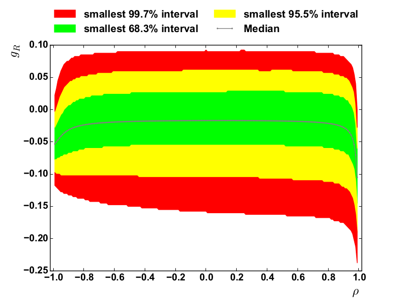
Figure 4: Contours of the smallest areas containing 68.3%, 95.5% and 99.7% posterior probability for $g_{R}$ as a function of the linear correlation coefficient $\rho$ between the measurements of $\sigma_{t}$ and $\sigma_{\bar{t}}$.

For the second interpretation, we assume all four couplings to be free parameters of the fit. As an example, Figs. 5, Fig. 6 and Fig. 7 show the marginal posterior distributions in the $(V_{L},V_{R})$-plane, in the $(V_{L},g_{R})$-plane, and in the $(g_{L},g_{R})$-plane, respectively. All three distributions have highly non-Gaussian shapes and some show disconnected regions. In each of the projections, the local mode is consistent with the predictions of the SM and the absence of anomalous couplings.

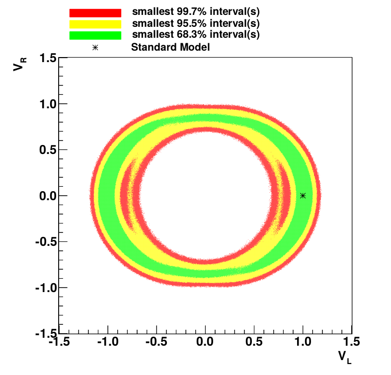
Figure 5: Marginal posterior distributions in the $(V_{L},V_{R})$-plane when all four parameters are left free in the fit and all four measurements are considered.

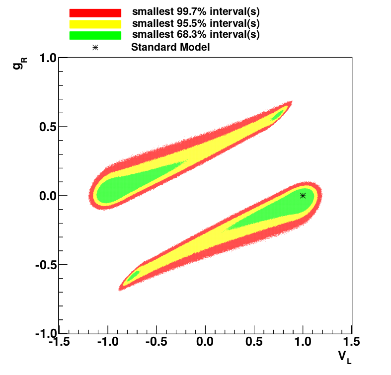
Figure 6: Marginal posterior distributions in the $(V_{L},g_{R})$-plane when all four parameters are left free in the fit and all four measurements are considered.

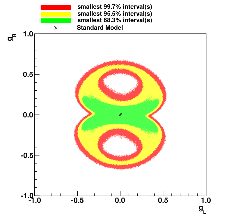
Figure 7: Marginal posterior distributions in the $(g_{L},g_{R})$-plane when all four parameters are left free in the fit and all four measurements are considered.

The global mode is found at $V_{L}=1.02$, $V_{R}=-0.06$, $g_{L}=0.03$, and $g_{R}=-0.01$. Since the smallest four-dimensional hypervolume containing 68.3% posterior probability is strongly non-Gaussian in shape and features several disconnected subsets, one-dimensional measures, such as the standard deviation or smallest intervals, are rendered useless.

6 Conclusions

We have presented a tool for interpreting measurements in the context of effective field theories. This EFTfitter allows implementing a user-defined model, either directly or via interfaces to other software tools, including predictions of observables based on the free parameters of the model. Measurements of these observables are then combined and used to constrain the free parameters. A variety of features of the EFTfitter helps to quantify and visualise the results. An example in the field of top-quark physics was shown, for which anomalous couplings of the $Wtb$-vertex were constrained based on measurements of the $W$-boson helicity fractions and the single-top $t$-channel cross sections.

- (1) F. Beaujean, C. Bobeth, D. van Dyk, Eur. Phys. J. C74, 2897 (2014). [Erratum: Eur. Phys. J. C74, 3179 (2014)]
- (2) P. Bechtle, K. Desch, P. Wienemann, Comput. Phys. Commun. 174, 47 (2006)
- (3) H. Flacher, et al., Eur. Phys. J. C60, 543 (2009). [Erratum: Eur. Phys. J. C71, 1718 (2011)]
- (4) M. Czakon, A. Mitov, JHEP 01, 080 (2013)
- (5) M. Czakon, A. Mitov, Comput. Phys. Commun. 185, 2930 (2014)
- (6) M. Czakon, P. Fiedler, A. Mitov, Phys. Rev. Lett. 110, 252004 (2013)
- (7) P. Langacker, M. Luo, Phys. Rev. D44, 817 (1991)
- (8) R.T. Bayes, Phil. Trans. Roy. Soc. Lond. 53, 370 (1764)
- (9) A. Valassi, Nucl. Instrum. Meth. A500, 391 (2003)
- (10) L. Lyons, D. Gibaut, P. Clifford, Nucl. Instrum. Meth. A270, 110 (1988)
- (11) S. Brandt, Data Analysis - Statistical and Computational Methods for Scientists and Engineers (Springer, 1999)
- (12) T. Leonard, J. Hsu, Ann. Stat. 20, 1669 (1992)
- (13) J. Barnard, R. McCulloch, X.L. Meng, Stat. Sinica 10, 1281 (2000)
- (14) A. Huang, M. Wand, Bayesian Anal. 8, 439 (2013)
- (15) A. Caldwell, D. Kollar, K. Kröninger, Comput. Phys. Commun. 180, 2197 (2009)
- (16) R. Brun, F. Rademakers, Nucl. Instrum. Meth. A389, 81 (1997)
- (17) J.A. Aguilar-Saavedra, et al., Eur. Phys. J. C50, 519 (2007)
- (18) J.A. Aguilar-Saavedra, Nucl. Phys. B804, 160 (2008)
- (19) J.A. Aguilar-Saavedra, Nucl. Phys. B812, 181 (2009)
- (20) C. Zhang, S. Willenbrock, Phys. Rev. D83, 034006 (2011)
- (21) A. Buckley, et al., Phys. Rev. D92, 091501 (2015)
- (22) A. Buckley, et al., JHEP 04, 015 (2016)
- (23) C. Bernardo, et al., Phys. Rev. D90, 113007 (2014)
- (24) M. Fabbrichesi, M. Pinamonti, A. Tonero, Eur. Phys. J. C74, 3193 (2014)
- (25) J.L. Birman, et al., (2016)
- (26) F. Bach, T. Ohl, Phys. Rev. D90, 074022 (2014)
- (27) A. Czarnecki, J.G. Korner, J.H. Piclum, Phys. Rev. D81, 111503 (2010)
- (28) N. Kidonakis, Phys. Rev. D83, 091503 (2011)
- (29) CMS Collaboration, JHEP 10, 167 (2013)
- (30) ATLAS Collaboration, Phys. Rev. D90, 112006 (2014)