Modelling Interaction of Sentence Pair with Coupled-LSTMs

Abstract

Recently, there is rising interest in modelling the interactions of two sentences with deep neural networks. However, most of the existing methods encode two sequences with separate encoders, in which a sentence is encoded with little or no information from the other sentence. In this paper, we propose a deep architecture to model the strong interaction of sentence pair with two coupled-LSTMs. Specifically, we introduce two coupled ways to model the interdependences of two LSTMs, coupling the local contextualized interactions of two sentences. We then aggregate these interactions and use a dynamic pooling to select the most informative features. Experiments on two very large datasets demonstrate the efficacy of our proposed architecture and its superiority to state-of-the-art methods.

1 Introduction

Distributed representations of words or sentences have been widely used in many natural language processing (NLP) tasks, such as text classification Kalchbrenner et al. (2014), question answering and machine translation Sutskever et al. (2014) and so on. Among these tasks, a common problem is modelling the relevance/similarity of the sentence pair, which is also called text semantic matching.

Recently, deep learning based models is rising a substantial interest in text semantic matching and have achieved some great progresses Hu et al. (2014); Qiu and Huang (2015); Wan et al. (2016).

According to the phases of interaction between two sentences, previous models can be classified into three categories.

Weak interaction Models

Some early works focus on sentence level interactions, such as ARC-IHu et al. (2014), CNTNQiu and Huang (2015) and so on. These models first encode two sequences with some basic (Neural Bag-of-words, BOW) or advanced (RNN, CNN) components of neural networks separately, and then compute the matching score based on the distributed vectors of two sentences. In this paradigm, two sentences have no interaction until arriving final phase.

Semi-interaction Models

Some improved methods focus on utilizing multi-granularity representation (word, phrase and sentence level), such as MultiGranCNN Yin and Schütze (2015) and Multi-Perspective CNN He et al. (2015). Another kind of models use soft attention mechanism to obtain the representation of one sentence by depending on representation of another sentence, such as ABCNN Yin et al. (2015), Attention LSTMRocktäschel et al. (2015); Hermann et al. (2015). These models can alleviate the weak interaction problem, but are still insufficient to model the contextualized interaction on the word as well as phrase level.

Strong Interaction Models

These models directly build an interaction space between two sentences and model the interaction at different positions. ARC-II Hu et al. (2014) and MV-LSTM Wan et al. (2016). These models enable the model to easily capture the difference between semantic capacity of two sentences.

In this paper, we propose a new deep neural network architecture to model the strong interactions of two sentences. Different with modelling two sentences with separated LSTMs, we utilize two interdependent LSTMs, called coupled-LSTMs, to fully affect each other at different time steps. The output of coupled-LSTMs at each step depends on both sentences. Specifically, we propose two interdependent ways for the coupled-LSTMs: loosely coupled model (LC-LSTMs) and tightly coupled model (TC-LSTMs). Similar to bidirectional LSTM for single sentence Schuster and Paliwal (1997); Graves and Schmidhuber (2005), there are four directions can be used in coupled-LSTMs. To utilize all the information of four directions of coupled-LSTMs, we aggregate them and adopt a dynamic pooling strategy to automatically select the most informative interaction signals. Finally, we feed them into a fully connected layer, followed by an output layer to compute the matching score.

The contributions of this paper can be summarized as follows.

1. Different with the architectures of using similarity matrix, our proposed architecture directly model the strong interactions of two sentences with coupled-LSTMs, which can capture the useful local semantic relevances of two sentences. Our architecture can also capture the multiple granular interactions by several stacked coupled-LSTMs layers.

2. Compared to the previous works on text matching, we perform extensive empirical studies on two very large datasets. The massive scale of the datasets allows us to train a very deep neural networks. Experiment results demonstrate that our proposed architecture is more effective than state-of-the-art methods.

2 Sentence Modelling with LSTM

Long short-term memory network (LSTM) Hochreiter and Schmidhuber (1997) is a type of recurrent neural network (RNN) Elman (1990), and specifically addresses the issue of learning long-term dependencies. LSTM maintains a memory cell that updates and exposes its content only when deemed necessary.

While there are numerous LSTM variants, here we use the LSTM architecture used by Jozefowicz et al. (2015), which is similar to the architecture of Graves (2013) but without peep-hole connections.

We define the LSTM units at each time step $t$ to be a collection of vectors in $\mathbb{R}^{d}$: an input gate $\mathbf{i}_{t}$, a forget gate $\mathbf{f}_{t}$, an output gate $\mathbf{o}_{t}$, a memory cell $\mathbf{c}_{t}$ and a hidden state $\mathbf{h}_{t}$. $d$ is the number of the LSTM units. The elements of the gating vectors $\mathbf{i}_{t}$, $\mathbf{f}_{t}$ and $\mathbf{o}_{t}$ are in $[0,1]$.

The LSTM is precisely specified as follows.

$$\begin{bmatrix}\mathbf{\tilde{c}}_{t}\\ \mathbf{o}_{t}\\ \mathbf{i}_{t}\\ \mathbf{f}_{t}\end{bmatrix} =\begin{bmatrix}\tanh\\ \sigma\\ \sigma\\ \sigma\end{bmatrix}T_{\mathbf{A},\mathbf{b}}\begin{bmatrix}\mathbf{x}_{t}\\ \mathbf{h}_{t-1}\end{bmatrix},$$ (1)

$$\mathbf{c}_{t} =\mathbf{\tilde{c}}_{t}\odot\mathbf{i}_{t}+\mathbf{c}_{t-1}\odot\mathbf{f}_{t},$$ (2)

$$\mathbf{h}_{t} =\mathbf{o}_{t}\odot\tanh\left(\mathbf{c}_{t}\right),$$ (3)

where $\mathbf{x}_{t}$ is the input at the current time step; $T_{\mathbf{A},\mathbf{b}}$ is an affine transformation which depends on parameters of the network $\mathbf{A}$ and $\mathbf{b}$. $\sigma$ denotes the logistic sigmoid function and $\odot$ denotes elementwise multiplication. Intuitively, the forget gate controls the amount of which each unit of the memory cell is erased, the input gate controls how much each unit is updated, and the output gate controls the exposure of the internal memory state.

The update of each LSTM unit can be written precisely as follows

$$(\mathbf{h}_{t},\mathbf{c}_{t}) =\mathbf{LSTM}(\mathbf{h}_{t-1},\mathbf{c}_{t-1},\mathbf{x}_{t}).$$ (4)

Here, the function $\mathbf{LSTM}(\cdot,\cdot,\cdot)$ is a shorthand for Eq. (1-3).

3 Coupled-LSTMs for Strong Sentence Interaction

To deal with two sentences, one straightforward method is to model them with two separate LSTMs. However, this method is difficult to model local interactions of two sentences. An improved way is to introduce attention mechanism, which has been used in many tasks, such as machine translation Bahdanau et al. (2014) and question answering Hermann et al. (2015).

Inspired by the multi-dimensional recurrent neural network Graves et al. (2007); Graves and Schmidhuber (2009); Byeon et al. (2015) and grid LSTM Kalchbrenner et al. (2015) in computer vision community, we propose two models to capture the interdependences between two parallel LSTMs, called coupled-LSTMs (C-LSTMs).

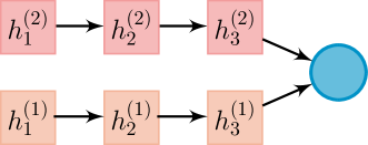
(a) Parallel LSTMs

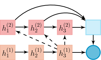
(b) Attention LSTMs

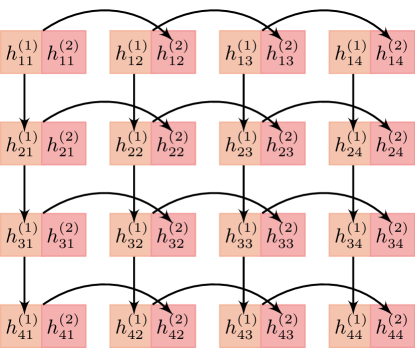
(c) Loosely coupled-LSTMs

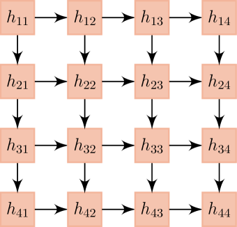
(d) Tightly coupled-LSTMs

Figure 1: Four different coupled-LSTMs.

To facilitate our models, we firstly give some definitions. Given two sequences $X=x_{1},x_{2},\cdots,x_{n}$ and $Y=y_{1},y_{2},\cdots,y_{m}$, we let $\mathbf{x}_{i}\in\mathbb{R}^{d}$ denote the embedded representation of the word $x_{i}$. The standard LSTM have one temporal dimension. When dealing with a sentence, LSTM regards the position as time step. At position $i$ of sentence $x_{1:n}$, the output $\mathbf{h}_{i}$ reflects the meaning of subsequence $x_{0:i}={x_{0},\cdots,x_{i}}$.

To model the interaction of two sentences as early as possible, we define $\mathbf{h}_{i,j}$ to represent the interaction of the subsequences $x_{0:i}$ and $y_{0:j}$.

Figure 1(c) and 1(d) illustrate our two propose models. For intuitive comparison of weak interaction parallel LSTMs, we also give parallel LSTMs and attention LSTMs in Figure 1(a) and 1(b).

We describe our two proposed models as follows.

3.1 Loosely Coupled-LSTMs (LC-LSTMs)

To model the local contextual interactions of two sentences, we enable two LSTMs to be interdependent at different positions. Inspired by Grid LSTM Kalchbrenner et al. (2015) and word-by-word attention LSTMs Rocktäschel et al. (2015), we propose a loosely coupling model for two interdependent LSTMs.

More concretely, we refer to $\mathbf{h}_{i,j}^{(1)}$ as the encoding of subsequence $x_{0:i}$ in the first LSTM influenced by the output of the second LSTM on subsequence $y_{0:j}$. Meanwhile, $\mathbf{h}_{i,j}^{(2)}$ is the encoding of subsequence $y_{0:j}$ in the second LSTM influenced by the output of the first LSTM on subsequence $x_{0:i}$

$\mathbf{h}_{i,j}^{(1)}$ and $\mathbf{h}_{i,j}^{(2)}$ are computed as

$$\mathbf{h}_{i,j}^{(1)} =\mathbf{LSTM}^{1}(\mathbf{H}_{i-1}^{(1)},\mathbf{c}_{i-1,j}^{(1)},\mathbf{\mathbf{x}}_{i}),$$ (5)

$$\mathbf{h}_{i,j}^{(2)} =\mathbf{LSTM}^{2}(\mathbf{H}_{j-1}^{(2)},\mathbf{c}_{i,j-1}^{(2)},\mathbf{y}_{j}),$$ (6)

where

$$\mathbf{H}_{i-1}^{(1)}=[\mathbf{h}_{i-1,j}^{(1)},\mathbf{h}_{i-1,j}^{(2)}],$$ (7)

$$\mathbf{H}_{j-1}^{(2)}=[\mathbf{h}_{i,j-1}^{(1)},\mathbf{h}_{i,j-1}^{(2)}].$$ (8)

3.2 Tightly Coupled-LSTMs (TC-LSTMs)

The hidden states of LC-LSTMs are the combination of the hidden states of two interdependent LSTMs, whose memory cells are separated. Inspired by the configuration of the multi-dimensional LSTM Byeon et al. (2015), we further conflate both the hidden states and the memory cells of two LSTMs. We assume that $\mathbf{h}_{i,j}$ directly model the interaction of the subsequences $x_{0:i}$ and $y_{0:j}$, which depends on two previous interaction $\mathbf{h}_{i-1,j}$ and $\mathbf{h}_{i,j-1}$, where $i,j$ are the positions in sentence $X$ and $Y$.

We define a tightly coupled-LSTMs units as follows.

$$\begin{bmatrix}\mathbf{\tilde{c}}_{i,j}\\ \mathbf{o}_{i,j}\\ \mathbf{i}_{i,j}\\ \mathbf{f}_{i,j}^{1}\\ \mathbf{f}_{i,j}^{2}\end{bmatrix} =\begin{bmatrix}\tanh\\ \sigma\\ \sigma\\ \sigma\\ \sigma\end{bmatrix}T_{\mathbf{A},\mathbf{b}}\begin{bmatrix}\mathbf{x}_{i}\\ \mathbf{y}_{j}\\ \mathbf{h}_{i,j-1}\\ \mathbf{h}_{i-1,j}\end{bmatrix},$$ (9)

$$\mathbf{c}_{i,j} =\mathbf{\tilde{c}}_{i,j}\odot\mathbf{i}_{i,j}+[\mathbf{c}_{i,j-1},\mathbf{c}_{i-1,j}]^{\mathrm{T}}\begin{bmatrix}\mathbf{f}_{i,j}^{1}\\ \mathbf{f}_{i,j}^{2}\\ \end{bmatrix}$$ (10)

$$\mathbf{h}_{i,j} =\mathbf{o}_{t}\odot\tanh\left(\mathbf{c}_{i,j}\right)$$ (11)

where the gating units $\mathbf{i}_{i,j}$ and $\mathbf{o}_{i,j}$ determine which memory units are affected by the inputs through $\mathbf{\tilde{c}}_{i,j}$, and which memory cells are written to the hidden units $\mathbf{h}_{i,j}$. $T_{\mathbf{A},\mathbf{b}}$ is an affine transformation which depends on parameters of the network $\mathbf{A}$ and $\mathbf{b}$. In contrast to the standard LSTM defined over time, each memory unit $\mathbf{c}_{i,j}$ of a tightly coupled-LSTMs has two preceding states $\mathbf{c}_{i,j-1}$ and $\mathbf{c}_{i-1,j}$ and two corresponding forget gates $\mathbf{f}_{i,j}^{1}$ and $\mathbf{f}_{i,j}^{2}$.

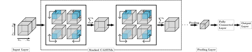
Figure 2: Architecture of coupled-LSTMs for sentence-pair encoding. Inputs are fed to four C-LSTMs followed by an aggregation layer. Blue cuboids represent different contextual information from four directions.

3.3 Analysis of Two Proposed Models

Our two proposed coupled-LSTMs can be formulated as

$$(\mathbf{h}_{i,j},\mathbf{c}_{i,j}) =\textbf{C-LSTMs}(\mathbf{h}_{i-1,j},\mathbf{h}_{i,j-1},\mathbf{c}_{i-1,j},\mathbf{c}_{i,j-1},\mathbf{x}_{i},\mathbf{y}_{j}),$$ (12)

where C-LSTMs can be either TC-LSTMs or LC-LSTMs.

The input consisted of two type of information at step $(i,j)$ in coupled-LSTMs: temporal dimension $\mathbf{h}_{i-1,j},\mathbf{h}_{i,j-1},\mathbf{c}_{i-1,j},\mathbf{c}_{i,j-1}$ and depth dimension $\mathbf{x}_{i},\mathbf{y}_{j}$. The difference between TC-LSTMs and LC-LSTMs is the dependence of information from temporal and depth dimension.

Interaction Between Temporal Dimensions

The TC-LSTMs model the interactions at position $(i,j)$ by merging the internal memory $\mathbf{c}_{i-1,j}$ $\mathbf{c}_{i,j-1}$ and hidden state $\mathbf{h}_{i-1,j}$ $\mathbf{h}_{i,j-1}$ along row and column dimensions. In contrast with TC-LSTMs, LC-LSTMs firstly use two standard LSTMs in parallel, producing hidden states $\mathbf{h}^{1}_{i,j}$ and $\mathbf{h}^{2}_{i,j}$ along row and column dimensions respectively, which are then merged together flowing next step.

Interaction Between Depth Dimension

In TC-LSTMs, each hidden state $\mathbf{h}_{i,j}$ at higher layer receives a fusion of information $\mathbf{x}_{i}$ and $\mathbf{y}_{j}$, flowed from lower layer. However, in LC-LSTMs, the information $\mathbf{x}_{i}$ and $\mathbf{y}_{j}$ are accepted by two corresponding LSTMs at the higher layer separately.

The two architectures have their own characteristics, TC-LSTMs give more strong interactions among different dimensions while LC-LSTMs ensures the two sequences interact closely without being conflated using two separated LSTMs.

3.3.1 Comparison of LC-LSTMs and word-by-word Attention LSTMs

The main idea of attention LSTMs is that the representation of sentence X is obtained dynamically based on the alignment degree between the words in sentence X and Y, which is asymmetric unidirectional encoding. Nevertheless, in LC-LSTM, each hidden state of each step is obtained with the consideration of interaction between two sequences with symmetrical encoding fashion.

4 End-to-End Architecture for Sentence Matching

In this section, we present an end-to-end deep architecture for matching two sentences, as shown in Figure 2.

4.1 Embedding Layer

To model the sentences with neural model, we firstly need transform the one-hot representation of word into the distributed representation. All words of two sequences $X=x_{1},x_{2},\cdots,x_{n}$ and $Y=y_{1},y_{2},\cdots,y_{m}$ will be mapped into low dimensional vector representations, which are taken as input of the network.

4.2 Stacked Coupled-LSTMs Layers

After the embedding layer, we use our proposed coupled-LSTMs to capture the strong interactions between two sentences. A basic block consists of five layers. We firstly use four directional coupled-LSTMs to model the local interactions with different information flows. And then we sum the outputs of these LSTMs by aggregation layer. To increase the learning capabilities of the coupled-LSTMs, we stack the basic block on top of each other.

4.2.1 Four Directional Coupled-LSTMs Layers

The C-LSTMs is defined along a certain pre-defined direction, we can extend them to access to the surrounding context in all directions. Similar to bi-directional LSTM, there are four directions in coupled-LSTMs.

$$(\mathbf{h}^{1}_{i,j},\mathbf{c}^{1}_{i,j}) =\textbf{C-LSTMs}(\mathbf{h}_{i-1,j},\mathbf{h}_{i,j-1},\mathbf{c}_{i-1,j},\mathbf{c}_{i,j-1},\mathbf{x}_{i},\mathbf{y}_{j}),$$

$$(\mathbf{h}^{2}_{i,j},\mathbf{c}^{2}_{i,j}) =\textbf{C-LSTMs}(\mathbf{h}_{i-1,j},\mathbf{h}_{i,j+1},\mathbf{c}_{i-1,j},\mathbf{c}_{i,j+1},\mathbf{x}_{i},\mathbf{y}_{j}),$$

$$(\mathbf{h}^{3}_{i,j},\mathbf{c}^{3}_{i,j}) =\textbf{C-LSTMs}(\mathbf{h}_{i+1,j},\mathbf{h}_{i,j+1},\mathbf{c}_{i+1,j},\mathbf{c}_{i,j+1},\mathbf{x}_{i},\mathbf{y}_{j}),$$

$$(\mathbf{h}^{4}_{i,j},\mathbf{c}^{4}_{i,j}) =\textbf{C-LSTMs}(\mathbf{h}_{i+1,j},\mathbf{h}_{i,j-1},\mathbf{c}_{i+1,j},\mathbf{c}_{i,j-1},\mathbf{x}_{i},\mathbf{y}_{j}).$$

4.2.2 Aggregation Layer

The aggregation layer sums the outputs of four directional coupled-LSTMs into a vector.

$$\hat{\mathbf{h}}_{i,j}=\sum_{d=1}^{4}\mathbf{h}_{i,j}^{d},$$ (13)

where the superscript $t$ of $\mathbf{h}_{i,j}$ denotes the different directions.

4.2.3 Stacking C-LSTMs Blocks

To increase the capabilities of network of learning multiple granularities of interactions, we stack several blocks (four C-LSTMs layers and one aggregation layer) to form deep architectures.

4.3 Pooling Layer

The output of stacked coupled-LSTMs layers is a tensor $\mathbf{H}\in\mathbb{R}^{n\times m\times d}$, where $n$ and $m$ are the lengths of sentences, and $d$ is the number of hidden neurons. We apply dynamic pooling to automatically extract $\mathbb{R}^{p\times q}$ subsampling matrix in each slice $\mathbf{H}_{i}\in\mathbb{R}^{n\times m}$, similar to Socher et al. (2011).

More formally, for each slice matrix $\mathbf{H}_{i}$, we partition the rows and columns of $\mathbf{H}_{i}$ into $p\times q$ roughly equal grids. These grid are non-overlapping. Then we select the maximum value within each grid. Since each slice $\mathbf{H}_{i}$ consists of the hidden states of one neuron at different positions, the pooling operation can be regarded as the most informative interactions captured by the neuron.

Thus, we get a $p\times q\times d$ tensor, which is further reshaped into a vector.

4.4 Fully-Connected Layer

The vector obtained by pooling layer is fed into a full connection layer to obtain a final more abstractive representation.

4.5 Output Layer

The output layer depends on the types of the tasks, we choose the corresponding form of output layer. There are two popular types of text matching tasks in NLP. One is ranking task, such as community question answering. Another is classification task, such as textual entailment.

1. For ranking task, the output is a scalar matching score, which is obtained by a linear transformation after the last fully-connected layer.

2. For classification task, the outputs are the probabilities of the different classes, which is computed by a softmax function after the last fully-connected layer.

5 Training

Our proposed architecture can deal with different sentence matching tasks. The loss functions varies with different tasks.

Max-Margin Loss for Ranking Task

Given a positive sentence pair $(X,Y)$ and its corresponding negative pair $(X,\hat{Y})$. The matching score $s(X,Y)$ should be larger than $s(X,\hat{Y})$.

For this task, we use the contrastive max-margin criterion Bordes et al. (2013); Socher et al. (2013) to train our models on matching task.

The ranking-based loss is defined as

$$L(X,Y,\hat{Y})=max(0,1-s(X,Y)+s(X,\hat{Y})).$$ (14)

where $s(X,Y)$ is predicted matching score for $(X,Y)$.

Cross-entropy Loss for Classification Task

Given a sentence pair $(X,Y)$ and its label $l$. The output $\hat{l}$ of neural network is the probabilities of the different classes. The parameters of the network are trained to minimise the cross-entropy of the predicted and true label distributions.

$$L(X,Y;\emph{{l}},\hat{\emph{{l}}})=-\sum_{j=1}^{C}\emph{{l}}_{j}\log(\hat{\emph{{l}}}_{j}),$$ (15)

where l is one-hot representation of the ground-truth label $l$; ${\hat{\emph{{l}}}}$ is predicted probabilities of labels; $C$ is the class number.

To minimize the objective, we use stochastic gradient descent with the diagonal variant of AdaGrad Duchi et al. (2011). To prevent exploding gradients, we perform gradient clipping by scaling the gradient when the norm exceeds a threshold Graves (2013).

6 Experiment

In this section, we investigate the empirical performances of our proposed model on two different text matching tasks: classification task (recognizing textual entailment) and ranking task (matching of question and answer).

	MQA	RTE
Embedding size	100	100
Hidden layer size	50	50
Initial learning rate	0.05	0.005
Regularization	$5E{-5}$	$1E{-5}$
Pooling $(p,q)$	(2,1)	(1,1)

Table 1: Hyper-parameters for our model on two tasks.

6.1 Hyperparameters and Training

The word embeddings for all of the models are initialized with the 100d GloVe vectors (840B token version, Pennington et al. (2014)) and fine-tuned during training to improve the performance. The other parameters are initialized by randomly sampling from uniform distribution in $[-0.1,0.1]$.

For each task, we take the hyperparameters which achieve the best performance on the development set via an small grid search over combinations of the initial learning rate $[0.05,0.0005,0.0001]$, $l_{2}$ regularization $[0.0,5E{-5},1E{-5},1E{-6}]$ and the threshold value of gradient norm [5, 10, 100]. The final hyper-parameters are set as Table 1.

6.2 Competitor Methods

• Neural bag-of-words (NBOW): Each sequence as the sum of the embeddings of the words it contains, then they are concatenated and fed to a MLP.

• Single LSTM: A single LSTM to encode the two sequences, which is used in Rocktäschel et al. (2015).

• Parallel LSTMs: Two sequences are encoded by two LSTMs separately, then they are concatenated and fed to a MLP.

• Attention LSTMs: An attentive LSTM to encode two sentences into a semantic space, which used in Rocktäschel et al. (2015).

• Word-by-word Attention LSTMs: An improvement of attention LSTM by introducing word-by-word attention mechanism, which used in Rocktäschel et al. (2015).

6.3 Experiment-I: Recognizing Textual Entailment

Recognizing textual entailment (RTE) is a task to determine the semantic relationship between two sentences. We use the Stanford Natural Language Inference Corpus (SNLI) Bowman et al. (2015). This corpus contains 570K sentence pairs, and all of the sentences and labels stem from human annotators. SNLI is two orders of magnitude larger than all other existing RTE corpora. Therefore, the massive scale of SNLI allows us to train powerful neural networks such as our proposed architecture in this paper.

Model	$k$	$|\theta|_{M}$	Train	Test
NBOW	100	80K	77.9	75.1
single LSTM Rocktäschel et al. (2015)	100	111K	83.7	80.9
parallel LSTMs Bowman et al. (2015)	100	221K	84.8	77.6
Attention LSTM Rocktäschel et al. (2015)	100	252K	83.2	82.3
Attention(w-by-w) LSTM Rocktäschel et al. (2015)	100	252K	83.7	83.5
LC-LSTMs (Single Direction)	50	45K	80.8	80.5
LC-LSTMs	50	45K	81.5	80.9
four stacked LC-LSTMs	50	135K	85.0	84.3
TC-LSTMs (Single Direction)	50	77.5K	81.4	80.1
TC-LSTMs	50	77.5K	82.2	81.6
four stacked TC-LSTMs	50	190K	86.7	85.1

Table 2: Results on SNLI corpus.

Index of Cell	Word or Phrase Pairs
$3$-th	(in a pool, swimming), (near a fountain, next to the ocean), (street, outside)
$9$-th	(doing a skateboard, skateboarding), (sidewalk with, inside), (standing, seated)
$17$-th	(blue jacket, blue jacket), (wearing black, wearing white), (green uniform, red uniform)
$25$-th	(a man, two other men), (a man, two girls), (an old woman, two people)

Table 3: Multiple interpretable neurons and the word-pairs/phrase-pairs captured by these neurons.

6.3.1 Results

Table 2 shows the evaluation results on SNLI. The $3$rd column of the table gives the number of parameters of different models without the word embeddings.

Our proposed two C-LSTMs models with four stacked blocks outperform all the competitor models, which indicates that our thinner and deeper network does work effectively.

Besides, we can see both LC-LSTMs and TC-LSTMs benefit from multi-directional layer, while the latter obtains more gains than the former. We attribute this discrepancy between two models to their different mechanisms of controlling the information flow from depth dimension.

Compared with attention LSTMs, our two models achieve comparable results to them using much fewer parameters (nearly $1/5$). By stacking C-LSTMs, the performance of them are improved significantly, and the four stacked TC-LSTMs achieve $85.1\%$ accuracy on this dataset.

Moreover, we can see TC-LSTMs achieve better performance than LC-LSTMs on this task, which need fine-grained reasoning over pairs of words as well as phrases.

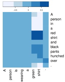
(a) 3rd neuron

(b) 17th neuron

Figure 3: Illustration of two interpretable neurons and some word-pairs capture by these neurons. The darker patches denote the corresponding activations are higher.

6.3.2 Understanding Behaviors of Neurons in C-LSTMs

To get an intuitive understanding of how the C-LSTMs work on this problem, we examined the neuron activations in the last aggregation layer while evaluating the test set using TC-LSTMs. We find that some cells are bound to certain roles.

Let $h_{i,j,k}$ denotes the activation of the $k$-th neuron at the position of $(i,j)$, where $i\in\{1,\ldots,n\}$ and $j\in\{1,\ldots,m\}$. By visualizing the hidden state $\mathbf{h}_{i,j,k}$ and analyzing the maximum activation, we can find that there exist multiple interpretable neurons. For example, when some contextualized local perspectives are semantically related at point $({i},{j})$ of the sentence pair, the activation value of hidden neuron $h_{{i},{j},k}$ tend to be maximum, meaning that the model could capture some reasoning patterns.

Figure 3 illustrates this phenomenon. In Figure 3(a), a neuron shows its ability to monitor the local contextual interactions about color. The activation in the patch, including the word pair “(red, green)”, is much higher than others. This is informative pattern for the relation prediction of these two sentences, whose ground truth is contradiction. An interesting thing is there are two words describing color in the sentence “ A person in a red shirt and black pants hunched over.”. Our model ignores the useless word “black”, which indicates that this neuron selectively captures pattern by contextual understanding, not just word level interaction.

In Figure 3(b), another neuron shows that it can capture the local contextual interactions, such as “(walking down the street, outside)”. These patterns can be easily captured by pooling layer and provide a strong support for the final prediction.

Table 3 illustrates multiple interpretable neurons and some representative word or phrase pairs which can activate these neurons. These cases show that our models can capture contextual interactions beyond word level.

6.3.3 Error Analysis

Although our models C-LSTMs are more sensitive to the discrepancy of the semantic capacity between two sentences, some semantic mistakes at the phrasal level still exist. For example, our models failed to capture the key informative pattern when predicting the entailment sentence pair “A girl takes off her shoes and eats blue cotton candy/The girl is eating while barefoot.”

Besides, despite the large size of the training corpus, it’s still very different to solve some cases, which depend on the combination of the world knowledge and context-sensitive inferences. For example, given an entailment pair “a man grabs his crotch during a political demonstration/The man is making a crude gesture”, all models predict “neutral”. This analysis suggests that some architectural improvements or external world knowledge are necessary to eliminate all errors instead of simply scaling up the basic model.

6.4 Experiment-II: Matching Question and Answer

Matching question answering (MQA) is a typical task for semantic matching. Given a question, we need select a correct answer from some candidate answers.

In this paper, we use the dataset collected from Yahoo! Answers with the getByCategory function provided in Yahoo! Answers API, which produces $963,072$ questions and corresponding best answers. We then select the pairs in which the length of questions and answers are both in the interval $[4,30]$, thus obtaining $220,000$ question answer pairs to form the positive pairs.

For negative pairs, we first use each question’s best answer as a query to retrieval top $1,000$ results from the whole answer set with Lucene, where $4$ or $9$ answers will be selected randomly to construct the negative pairs.

The whole dataset is divided into training, validation and testing data with proportion $20:1:1$. Moreover, we give two test settings: selecting the best answer from 5 and 10 candidates respectively.

Model	$k$	P@1(5)	P@1(10)
Random Guess	-	20.0	10.0
NBOW	50	63.9	47.6
single LSTM	50	68.2	53.9
parallel LSTMs	50	66.9	52.1
Attention LSTMs	50	73.5	62.0
LC-LSTMs (Single Direction)	50	75.4	63.0
LC-LSTMs	50	76.1	64.1
three stacked LC-LSTMs	50	78.5	66.2
TC-LSTMs (Single Direction)	50	74.3	62.4
TC-LSTMs	50	74.9	62.9
three stacked TC-LSTMs	50	77.0	65.3

Table 4: Results on Yahoo question-answer pairs dataset.

6.4.1 Results

Results of MQA are shown in the Table 4. For our models, due to stacking block more than three layers can not make significant improvements on this task, we just use three stacked C-LSTMs.

By analyzing the evaluation results of question-answer matching in table 4, we can see strong interaction models (attention LSTMs, our C-LSTMs) consistently outperform the weak interaction models (NBOW, parallel LSTMs) with a large margin, which suggests the importance of modelling strong interaction of two sentences.

Our proposed two C-LSTMs surpass the competitor methods and C-LSTMs augmented with multi-directions layers and multiple stacked blocks fully utilize multiple levels of abstraction to directly boost the performance.

Additionally, LC-LSTMs is superior to TC-LSTMs. The reason may be that MQA is a relative simple task, which requires less reasoning abilities, compared with RTE task. Moreover, the parameters of LC-LSTMs are less than TC-LSTMs, which ensures the former can avoid suffering from overfitting on a relatively smaller corpus.

7 Related Work

Our architecture for sentence pair encoding can be regarded as strong interaction models, which have been explored in previous models.

An intuitive paradigm is to compute similarities between all the words or phrases of the two sentences. Socher et al. [2011] firstly used this paradigm for paraphrase detection. The representations of words or phrases are learned based on recursive autoencoders. Wan et al. [2016] used LSTM to enhance the positional contextual interactions of the words or phrases between two sentences. The input of LSTM for one sentence does not involve another sentence.

A major limitation of this paradigm is the interaction of two sentence is captured by a pre-defined similarity measure. Thus, it is not easy to increase the depth of the network. Compared with this paradigm, we can stack our C-LSTMs to model multiple-granularity interactions of two sentences.

Rocktäschel et al. [2015] used two LSTMs equipped with attention mechanism to capture the iteration between two sentences. This architecture is asymmetrical for two sentences, where the obtained final representation is sensitive to the two sentences’ order.

Compared with the attentive LSTM, our proposed C-LSTMs are symmetrical and model the local contextual interaction of two sequences directly.

8 Conclusion and Future Work

In this paper, we propose an end-to-end deep architecture to capture the strong interaction information of sentence pair. Experiments on two large scale text matching tasks demonstrate the efficacy of our proposed model and its superiority to competitor models. Besides, our visualization analysis revealed that multiple interpretable neurons in our proposed models can capture the contextual interactions of the words or phrases.

In future work, we would like to incorporate some gating strategies into the depth dimension of our proposed models, like highway or residual network, to enhance the interactions between depth and other dimensions thus training more deep and powerful neural networks.

References

- Bahdanau et al. [2014] D. Bahdanau, K. Cho, and Y. Bengio. Neural machine translation by jointly learning to align and translate. ArXiv e-prints, September 2014.
- Bordes et al. [2013] Antoine Bordes, Nicolas Usunier, Alberto Garcia-Duran, Jason Weston, and Oksana Yakhnenko. Translating embeddings for modeling multi-relational data. In NIPS, 2013.
- Bowman et al. [2015] Samuel R. Bowman, Gabor Angeli, Christopher Potts, and Christopher D. Manning. A large annotated corpus for learning natural language inference. In Proceedings of the 2015 Conference on Empirical Methods in Natural Language Processing, 2015.
- Byeon et al. [2015] Wonmin Byeon, Thomas M Breuel, Federico Raue, and Marcus Liwicki. Scene labeling with lstm recurrent neural networks. In Proceedings of the IEEE Conference on Computer Vision and Pattern Recognition, pages 3547–3555, 2015.
- Duchi et al. [2011] John Duchi, Elad Hazan, and Yoram Singer. Adaptive subgradient methods for online learning and stochastic optimization. The Journal of Machine Learning Research, 12:2121–2159, 2011.
- Elman [1990] Jeffrey L Elman. Finding structure in time. Cognitive science, 14(2):179–211, 1990.
- Graves and Schmidhuber [2005] Alex Graves and Jürgen Schmidhuber. Framewise phoneme classification with bidirectional lstm and other neural network architectures. Neural Networks, 18(5):602–610, 2005.
- Graves and Schmidhuber [2009] Alex Graves and Jürgen Schmidhuber. Offline handwriting recognition with multidimensional recurrent neural networks. In Advances in Neural Information Processing Systems, pages 545–552, 2009.
- Graves et al. [2007] Alex Graves, Santiago Fernández, and Jürgen Schmidhuber. Multi-dimensional recurrent neural networks. In Artificial Neural Networks–ICANN 2007, pages 549–558. Springer, 2007.
- Graves [2013] Alex Graves. Generating sequences with recurrent neural networks. arXiv preprint arXiv:1308.0850, 2013.
- He et al. [2015] Hua He, Kevin Gimpel, and Jimmy Lin. Multi-perspective sentence similarity modeling with convolutional neural networks. In Proceedings of the 2015 Conference on Empirical Methods in Natural Language Processing, pages 1576–1586, 2015.
- Hermann et al. [2015] Karl Moritz Hermann, Tomas Kocisky, Edward Grefenstette, Lasse Espeholt, Will Kay, Mustafa Suleyman, and Phil Blunsom. Teaching machines to read and comprehend. In Advances in Neural Information Processing Systems, pages 1684–1692, 2015.
- Hochreiter and Schmidhuber [1997] Sepp Hochreiter and Jürgen Schmidhuber. Long short-term memory. Neural computation, 9(8):1735–1780, 1997.
- Hu et al. [2014] Baotian Hu, Zhengdong Lu, Hang Li, and Qingcai Chen. Convolutional neural network architectures for matching natural language sentences. In Advances in Neural Information Processing Systems, 2014.
- Jozefowicz et al. [2015] Rafal Jozefowicz, Wojciech Zaremba, and Ilya Sutskever. An empirical exploration of recurrent network architectures. In Proceedings of The 32nd International Conference on Machine Learning, 2015.
- Kalchbrenner et al. [2014] Nal Kalchbrenner, Edward Grefenstette, and Phil Blunsom. A convolutional neural network for modelling sentences. In Proceedings of ACL, 2014.
- Kalchbrenner et al. [2015] Nal Kalchbrenner, Ivo Danihelka, and Alex Graves. Grid long short-term memory. arXiv preprint arXiv:1507.01526, 2015.
- Pennington et al. [2014] Jeffrey Pennington, Richard Socher, and Christopher D Manning. Glove: Global vectors for word representation. Proceedings of the Empiricial Methods in Natural Language Processing (EMNLP 2014), 12:1532–1543, 2014.
- Qiu and Huang [2015] Xipeng Qiu and Xuanjing Huang. Convolutional neural tensor network architecture for community-based question answering. In Proceedings of International Joint Conference on Artificial Intelligence, 2015.
- Rocktäschel et al. [2015] Tim Rocktäschel, Edward Grefenstette, Karl Moritz Hermann, Tomáš Kočiskỳ, and Phil Blunsom. Reasoning about entailment with neural attention. arXiv preprint arXiv:1509.06664, 2015.
- Schuster and Paliwal [1997] Mike Schuster and Kuldip K Paliwal. Bidirectional recurrent neural networks. Signal Processing, IEEE Transactions on, 45(11):2673–2681, 1997.
- Socher et al. [2011] Richard Socher, Eric H Huang, Jeffrey Pennin, Christopher D Manning, and Andrew Y Ng. Dynamic pooling and unfolding recursive autoencoders for paraphrase detection. In Advances in Neural Information Processing Systems, 2011.
- Socher et al. [2013] Richard Socher, Danqi Chen, Christopher D Manning, and Andrew Ng. Reasoning with neural tensor networks for knowledge base completion. In Advances in Neural Information Processing Systems, pages 926–934, 2013.
- Sutskever et al. [2014] Ilya Sutskever, Oriol Vinyals, and Quoc VV Le. Sequence to sequence learning with neural networks. In Advances in Neural Information Processing Systems, pages 3104–3112, 2014.
- Wan et al. [2016] Shengxian Wan, Yanyan Lan, Jiafeng Guo, Jun Xu, Liang Pang, and Xueqi Cheng. A deep architecture for semantic matching with multiple positional sentence representations. In AAAI, 2016.
- Yin and Schütze [2015] Wenpeng Yin and Hinrich Schütze. Convolutional neural network for paraphrase identification. In Proceedings of the 2015 Conference of the North American Chapter of the Association for Computational Linguistics: Human Language Technologies, pages 901–911, 2015.
- Yin et al. [2015] Wenpeng Yin, Hinrich Schütze, Bing Xiang, and Bowen Zhou. Abcnn: Attention-based convolutional neural network for modeling sentence pairs. arXiv preprint arXiv:1512.05193, 2015.