Pairing mechanism of unconventional superconductivity in doped Kane-Mele model

Abstract

We study the pairing symmetry of a doped Kane-Mele model on a honeycomb lattice with on-site Coulomb interaction. The pairing instability of Cooper pair is calculated based on the linearized $\acute{\mathrm{E}}$liashberg equation within the random phase approximation (RPA). When the magnitude of the spin-orbit coupling is weak, even-frequency spin-singlet even-parity (ESE) pairing is dominant. On the other hand, with the increase of the spin-orbit coupling, we show that the even-frequency spin-triplet odd-parity (ETO) $f$-wave pairing exceeds ESE one. ETO $f$-wave pairing is supported by the longitudinal spin fluctuation. Since the transverse spin fluctuation is strongly suppressed by spin-orbit coupling, ETO $f$-wave pairing becomes dominant for large magnitude of spin-orbit coupling.

1 Introduction

To explore unconventional pairing in superconductivity has been an important issue in condensed matter physics[1]. It is known that $d$-wave pairing has been realized in high $T_{\mathrm{c}}$ cuprate [2, 3, 4, 5] and there have been many remarkable quantum phenomena specific to unconventional pairing having sign changes of gap function on the Fermi surface [2, 6, 7]. There are several strongly correlated systems where spin-singlet $d$-wave pairing are realized. On the other hand, spin-triplet $p$-wave pairing is realized in superfluid ³He [8]. In solid state materials, pairing symmetry of Sr₂RuO₄ is believed to be spin-triplet $p$-wave pairing [9].

As a natural extension of these anisotropic pairing, spin-triplet $f$-wave pairing has been also proposed [10, 11, 12, 13, 14, 15, 16]. Since $f$-wave pairing has a higher angular momentum, its gap function must have sign changes much more as compared to $d$-wave and $p$-wave pairings. Thus, it cannot be stable due to the presence of many nodes on the Fermi surface as far as we are considering simple Fermi surface located around the $\Gamma$ point. However, as proposed by Kuroki $et.$ $al.$, $f$-wave pairing is possible if we consider disconnected Fermi surfaces since the gap nodes do not have to cross the Fermi surface [10].

One of the possible systems is quasi one-dimensional organic superconductor (TMTSF)₂X (X=PF₆, ClO₄, etc. ). [17] A remarkable feature of this system is the coexistence of 2k_F charge density wave and 2k_F spin density wave (SDW). Then, the charge fluctuation becomes important and it favors the realization of spin-triplet pairing [11, 16]. Based on a fluctuation mediated pairing mechanism, $d$-wave and $f$-wave pairings become possible candidates. There have been several theoretical studies which support realization of spin-triplet $f$-wave pairing [11, 18, 19, 16, 20, 21, 22].

Another possibility of $f$-wave pairing was intensively discussed just after the discovery of superconductivity in $\mathrm{Na}_{x}$CoO₂ $\cdot$ $y$H₂O [23]. A triangular lattice structure of this material can host the disconnected Fermi surface around the K and K’ points. Spin-triplet $f$-wave pairing was proposed based on the fluctuation exchange method [12, 24]. Although there have been several theories supporting $f$-wave pairing [15, 13, 14, 25, 26, 27, 28], due to the presence of conflicting results[29, 30, 31], the pairing mechanism of this material is still controversial.

Other than these materials, there are several unconventional superconductors, $e.g.$, UPt₃ [32, 33] and SrPtAs [34, 35], where the possibility of spin-triplet $f$-wave pairing has been suggested. Also, in optical lattice systems, spin-triplet $f$-wave pairing has been proposed [36]. In the light of the preexisting theories, to explore spin-triplet $f$-wave pairing in hexagonal structures [37, 38, 39, 40, 41] is a challenging issue.

Recently, Zhang $et.$ $al.$ proposed that spin-triplet $f$-wave pairing is possible in doped silicene by applying an electric field [42]. Silicene, single atomic layer of Si forming a 2D honeycomb lattice like graphene[43], becomes a topical material from the view points of monolayer material and topological insulator. Nowadays, there are several works to explore unconventional superconductivity in atomic layered systems [44, 45, 46, 47, 48, 49]. Thus, to study the superconductivity in doped Kane-Mele model is interesting since it is a canonical model of monolayer systems with non-trivial topological property[50, 51]. We naively expect that the spin-orbit coupling may help the generation of spin-triplet pairing.

In this paper, we study the pairing instability of Cooper pair in doped Kane-Mele model with on-site Coulomb interaction by the linearized $\acute{\mathrm{E}}$liashberg equation within the random phase approximation (RPA). We clarify that even-frequency spin-singlet even-parity (ESE) pairing is dominant when the magnitude of the spin-orbit coupling is weak. On the other hand, with the increase of the spin-orbit coupling, we show that even-frequency spin-triplet odd-parity (ETO) $f$-wave pairing becomes dominant. We clarify physical reasons why $f$-wave pairing is realized.

The organization of this paper is as follows. In section II, we show a model Hamiltonian and formulations of the pairing interaction within RPA. An $\acute{\mathrm{E}}$liashberg equation is also formulated. In section III, we show calculated results of the $\acute{\mathrm{E}}$liashberg equation and discuss the pairing mechanism. In section IV, we summarize our results.

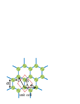
Figure 1: The structure of a honeycomb lattice. The dotted line denotes the unit cell where $\bm{a}_{1}$ and $\bm{a}_{2}$ are the lattice vectors. Each unit cell contains two sublattice $A$ and $B$ with distance $a$.

2 Model and Formulation

2.1 Hamiltonian

In this section, we introduce a model Hamiltonian and the formulations of the $\acute{\mathrm{E}}$liashberg equation to calculate the instabilities of the Cooper pairs. We consider the honeycomb lattice as shown in Fig. 1. Here, we take lattice vectors as ${\bm{a}}_{1}=(\sqrt{3}a,0)$ and ${\bm{a}_{2}}=(-\sqrt{3}a/2,3a/2)$. On this lattice, we consider a Kane-Mele model[50, 51],

$$\mathcal{H}_{0}=\sum_{\bm{k}\sigma}\hat{c}^{{\dagger}}_{\bm{k}\sigma}\hat{H}_{\sigma}(\bm{k})\hat{c}_{\bm{k}\sigma},$$ (1)

$$\hat{H}_{\sigma}(\bm{k})=$$

$$\begin{pmatrix}-\mu+(\sigma_{z})_{\sigma\sigma}\lambda_{\mathrm{SO}}W_{\mathrm{SO}}(\bm{k})&tW(\bm{k})\\ tW^{*}(\bm{k})&-\mu-(\sigma_{z})_{\sigma\sigma}\lambda_{\mathrm{SO}}W_{\mathrm{SO}}(\bm{k})\end{pmatrix},$$ (2)

$$W({\bm{k}})=(1+e^{-i\bm{k}\cdot{\bm{a}}_{2}}+e^{-i\bm{k}\cdot({\bm{a}}_{1}+{\bm{a}}_{2})}),$$ (3)

$$W_{\mathrm{SO}}({\bm{k}})=\frac{2}{3\sqrt{3}}\{\sin\bm{k}\cdot{\bm{a}}_{1}+\sin\bm{k}\cdot{\bm{a}}_{2}-\sin\bm{k}\cdot({\bm{a}}_{1}+{\bm{a}}_{2})\},$$ (4)

where $\hat{c}^{\dagger}_{\bm{k}\sigma}=(c^{\dagger}_{\bm{k}A\sigma}\ c^{\dagger}_{\bm{k}B\sigma})$ and $\hat{c}_{\bm{k}\sigma}=(c_{\bm{k}A\sigma}\ c_{\bm{k}B\sigma})^{T}$ are creation and annihilation operators of the electron with momentum ${\bm{k}}$ and spin $\sigma$ ($\sigma=\uparrow$ or $\downarrow$) on sublattice $A$ and $B$. $\mu$, $t$ and $\lambda_{\mathrm{SO}}$ denote the chemical potential, the nearest-neighbor hopping and the intrinsic spin-orbit interaction, respectively. $\sigma_{z}$ is the Pauli matrix in spin space. By diagonalizing $\hat{H}_{\sigma}(\bm{k})$, we obtain the dispersion relation in the normal state,

$$E_{\sigma}^{\pm}(\bm{k})=-\mu\pm\sqrt{t^{2}|W(\bm{k})|^{2}+\lambda_{\mathrm{SO}}^{2}W_{\mathrm{SO}}(\bm{k})^{2}}.$$ (5)

Since the spin-orbit interaction considered in the present model does not break the inversion symmetry and the time-reversal symmetry, the energy bands are doubly degenerated. In other words, $E_{\sigma}^{\pm}(\bm{k})$ does not depend on $\sigma$. Without the spin-orbit interaction $\lambda_{\mathrm{SO}}$, the valence bands and the conduction bands touch at the K and K’ points because $W(\bm{k})=0$ there. However, $\lambda_{\mathrm{SO}}$ makes band gaps as shown in Fig. 2.

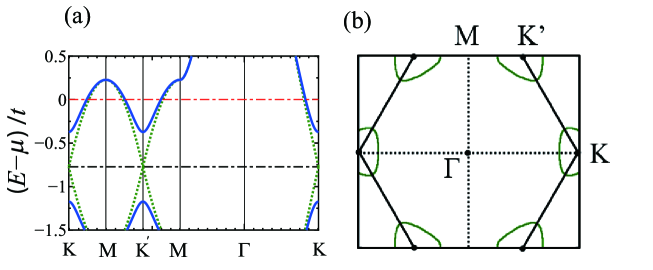
Figure 2: (a)The dispersion relation at $\lambda_{\mathrm{SO}}/t=$0 (dotted lines) and 0.4 (solid lines). $\mu/t=0.77$ for both cases. (b)Fermi surface in the normal states at $\lambda_{\mathrm{SO}}/t=$0.4 and $\mu/t=0.77$. The hexagonal line shows the first Brillouin zone.

To study the superconductivity in this system, we consider slightly carrier doped metallic state in the conduction bands. In this paper, we choose $\mu$ as the number of carrier in the conduction bands becomes 0.1 in each spin component. The obtained Fermi surfaces at $\lambda_{\mathrm{SO}}/t=0.4$ are shown in Fig. 2(b). As seen in the figure, two disconnected electron-pockets are formed at the K and K’ points. The shape of the Fermi surfaces is almost the same for other values of $\lambda_{\mathrm{SO}}$ used in the present paper, and the above character does not change.

As well as the non-interacting term in Eq. (1), we introduce the on-site repulsive interaction,

$$\mathcal{H}_{I} =\frac{U}{N}\sum_{{\bm{k}}{\bm{k}}^{\prime}{\bm{q}}\alpha}c^{\dagger}_{\bm{k+q}\alpha\uparrow}c^{\dagger}_{\bm{k^{\prime}-q}\alpha\downarrow}c_{\bm{k^{\prime}}\alpha\downarrow}c_{\bm{k}\alpha\uparrow}.$$ (6)

Here, $U$ and $N$ represent the on-site repulsive interaction and the system size. This interaction is treated by RPA.

2.2 Susceptibilities and effective pairing interactions

In this subsection, we calculate susceptibilities and resulting pairing interactions in the framework of RPA. For this purpose, we introduce the non-interacting temperature Green’s function,

$$\hat{G}^{\sigma}(\bm{k},i\varepsilon_{n}) =(i\varepsilon_{n}-H_{\sigma}(\bm{k}))^{-1}$$

$$=\begin{pmatrix}G_{AA}^{\sigma}(\bm{k},i\varepsilon_{n})&G_{AB}^{\sigma}(\bm{k},i\varepsilon_{n})\\ G_{BA}^{\sigma}(\bm{k},i\varepsilon_{n})&G_{BB}^{\sigma}(\bm{k},i\varepsilon_{n})\end{pmatrix},$$ (7)

where $\varepsilon_{n}=(2n+1)\pi k_{\mathrm{B}}T$ is a fermionic Matsubara frequency. Then, the irreducible susceptibilities are given by

$$\chi_{\alpha\beta;\gamma\delta}^{\sigma\tau}(\bm{q},i\omega_{m}) =-\frac{k_{\mathrm{B}}T}{N}\sum_{\bm{k},i\varepsilon_{n}}G_{\alpha\gamma}^{\sigma}(\bm{k}+\bm{q},i\varepsilon_{n}+i\omega_{m})G_{\delta\beta}^{\tau}(\bm{k},i\varepsilon_{n}),$$ (8)

where $\omega_{m}=2m\pi k_{\mathrm{B}}T$ is a bosonic Matsubara frequency. $\alpha$, $\beta$, $\gamma$ and $\delta$ ($\sigma$ and $\tau$) indicate sublattice (spin) indeces. From these irreducible susceptibilities, we construct bubble and ladder-type diagrams to calculate the spin and charge susceptibilities,

$$\chi_{\alpha\sigma,\beta\tau}^{\mathrm{B}}(\bm{q},i\omega_{m})$$

$$=\delta_{\sigma\tau}\chi_{\alpha\alpha;\beta\beta}^{\sigma\sigma}(\bm{q},i\omega_{m})-\sum_{\gamma}\chi_{\alpha\alpha;\gamma\gamma}^{\sigma\sigma}(\bm{q},i\omega_{m})U\chi_{\gamma\bar{\sigma},\beta\tau}^{\mathrm{B}}(\bm{q},i\omega_{m}),$$ (9)

$$\chi_{\alpha\sigma,\beta\sigma}^{\mathrm{L}}(\bm{q},i\omega_{m})$$

$$=\chi_{\alpha\alpha;\beta\beta}^{\sigma\bar{\sigma}}(\bm{q},i\omega_{m})+\sum_{\gamma}\chi_{\alpha\alpha;\gamma\gamma}^{\sigma\bar{\sigma}}(\bm{q},i\omega_{m})U\chi_{\gamma\sigma,\beta\sigma}^{\mathrm{L}}(\bm{q},i\omega_{m}),$$ (10)

where $\bar{\sigma}=\uparrow$ and $\downarrow$ for $\sigma=\downarrow$ and $\uparrow$, respectively. Note that $\chi_{\alpha\sigma,\beta\bar{\sigma}}^{\mathrm{L}}(\bm{q},i\omega_{m})$ with $\sigma\neq\bar{\sigma}$ are absent since there is no spin-flipping term in the non-perturbative Hamiltonian and on-site interaction acts between electrons with opposite spins. By solving simultaneous equations in Eqs. (9) and (10), we obtain $\chi_{\alpha\sigma,\beta\tau}^{\mathrm{B}}(\bm{q},i\omega_{m})$ and $\chi_{\alpha\sigma,\beta\sigma}^{\mathrm{L}}(\bm{q},i\omega_{m})$ as,

$$\chi_{\alpha\sigma,\alpha\sigma}^{\mathrm{B}}=(\chi_{\alpha\sigma,\alpha\sigma}^{\mathrm{B0}}+U^{2}\chi_{\bar{\alpha}\bar{\sigma},\bar{\alpha}\bar{\sigma}}^{\mathrm{B0}}\phi^{\mathrm{B0}}_{\sigma})/D^{\mathrm{B}},$$ (11)

$$\chi_{\alpha\sigma,\bar{\alpha}\sigma}^{\mathrm{B}}=(\chi_{\alpha\sigma,\bar{\alpha}\sigma}^{\mathrm{B0}}-U^{2}\chi_{\alpha\bar{\sigma},\bar{\alpha}\bar{\sigma}}^{\mathrm{B0}}\phi^{\mathrm{B0}}_{\sigma})/D^{\mathrm{B}},$$ (12)

$$\chi_{\alpha\sigma,\alpha\bar{\sigma}}^{\mathrm{B}}=\left(-U\sum_{\beta}\chi_{\alpha\sigma,\beta\sigma}^{\mathrm{B0}}\chi_{\beta\bar{\sigma},\alpha\bar{\sigma}}^{\mathrm{B0}}+U^{3}\Phi^{\mathrm{B0}}\right)/D^{\mathrm{B}},$$ (13)

$$\chi_{\alpha\sigma,\bar{\alpha}\bar{\sigma}}^{\mathrm{B}}=\left(-U\sum_{\beta}\chi_{\alpha\sigma,\beta\sigma}^{\mathrm{B0}}\chi_{\beta\bar{\sigma},\bar{\alpha}\bar{\sigma}}^{\mathrm{B0}}\right)/D^{\mathrm{B}},$$ (14)

with

$$\chi_{\alpha\sigma,\beta\sigma}^{\mathrm{B0}} =\chi_{\alpha\alpha;\beta\beta}^{\sigma\sigma},$$ (16)

$$D^{\mathrm{B}} =1-U^{2}\sum_{\alpha\beta}\chi_{\alpha\uparrow,\beta\uparrow}^{\mathrm{B0}}\chi_{\beta\downarrow,\alpha\downarrow}^{\mathrm{B0}}+U^{4}\Phi^{\mathrm{B0}},$$ (17)

$$\phi^{\mathrm{B0}}_{\sigma} =\chi_{A\sigma,B\sigma}^{\mathrm{B0}}\chi_{B\sigma,A\sigma}^{\mathrm{B0}}-\chi_{A\sigma,A\sigma}^{\mathrm{B0}}\chi_{B\sigma,B\sigma}^{\mathrm{B0}},$$ (18)

$$\Phi^{\mathrm{B0}} =\phi^{\mathrm{B0}}_{\uparrow}\phi^{\mathrm{B0}}_{\downarrow},$$ (19)

and

$$\chi_{\alpha\sigma,\alpha\sigma}^{\mathrm{L}}=(\chi_{\alpha\sigma,\alpha\sigma}^{\mathrm{L0}}+U\phi^{\mathrm{L0}}_{\sigma})/D^{\mathrm{L}}_{\sigma},$$ (20)

$$\chi_{\alpha\sigma,\bar{\alpha}\sigma}^{\mathrm{L}}=\chi_{\alpha\sigma,\bar{\alpha}\sigma}^{\mathrm{L0}}/D^{\mathrm{L}}_{\sigma},$$ (21)

with

$$\chi_{\alpha\sigma,\beta\sigma}^{\mathrm{L0}} =\chi_{\alpha\alpha;\beta\beta}^{\sigma\bar{\sigma}},$$ (22)

$$\phi^{\mathrm{L0}}_{\sigma} =\chi_{A\sigma,B\sigma}^{\mathrm{L0}}\chi_{B\sigma,A\sigma}^{\mathrm{L0}}-\chi_{A\sigma,A\sigma}^{\mathrm{L0}}\chi_{B\sigma,B\sigma}^{\mathrm{L0}},$$ (23)

$$D^{\mathrm{L}}_{\sigma} =1-U\sum_{\alpha}\chi_{\alpha\sigma,\alpha\sigma}^{\mathrm{L0}}-U^{2}\phi^{\mathrm{L0}}_{\sigma},$$ (24)

where we abbreviate the variable $\bm{q}$ and $i\omega_{m}$. Then, we derive the longitudinal and transverse spin and charge susceptibilities,

$$\chi^{zz}_{\alpha\beta}(\bm{q},i\omega_{m})=\frac{1}{4}\sum_{\sigma}(\chi_{\alpha\sigma,\beta\sigma}^{\mathrm{B}}(\bm{q},i\omega_{m})-\chi_{\alpha\sigma,\beta\bar{\sigma}}^{\mathrm{B}}(\bm{q},i\omega_{m})),$$ (25)

$$\chi^{+-}_{\alpha\beta}(\bm{q},i\omega_{m})=\chi_{\alpha\sigma,\beta\sigma}^{\mathrm{L}}(\bm{q},i\omega_{m}),$$ (26)

$$\chi^{\mathrm{C}}_{\alpha\beta}(\bm{q},i\omega_{m})=\frac{1}{2}\sum_{\sigma\sigma^{\prime}}\chi_{\alpha\sigma,\beta\sigma^{\prime}}^{\mathrm{B}}(\bm{q},i\omega_{m}),$$ (27)

where $\chi^{zz}_{\alpha\beta}(\bm{q},i\omega_{m})$, $\chi^{+-}_{\alpha\beta}(\bm{q},i\omega_{m})$ and $\chi^{\mathrm{C}}_{\alpha\beta}(\bm{q},i\omega_{m})$ denote longitudinal spin, transverse spin and charge susceptibilities, respectively. Without the spin-orbit interaction, spin rotational symmetry leads to the relation $\chi^{+-}_{\alpha\beta}(\bm{q},i\omega_{m})=2\chi^{zz}_{\alpha\beta}(\bm{q},i\omega_{m})$. However, this relation is broken in the presence of spin-orbit interaction. When $D^{\mathrm{B}}$ ($D^{\mathrm{L}}_{\sigma}$) becomes 0, longitudinal (transverse) spin susceptibility diverges. In other words, we can determine the critical temperature for magnetic instability by solving these equations.

2.3 Linearized $\acute{E}$liashberg equation

In this subsection, we introduce the $\acute{\mathrm{E}}$liashberg equation to discuss the pairing instability. The $\acute{\mathrm{E}}$liashberg equation is used to determine the critical temperature $T_{\mathrm{c}}$ of superconductivity and gap function just below $T_{\mathrm{c}}$. In this temperature region, the gap function and the anomalous Green’s function can be linearized in the Dyson-Gor’kov equation. Then, the Dyson-Gor’kov equation can be reduced to the eigenvalue equation. This eigenvalue equation is called the $\acute{\mathrm{E}}$liashberg equation given by

$$\lambda\Delta_{\alpha\sigma,\beta\tau}(\bm{k},i\varepsilon_{n})$$

$$=-\frac{k_{B}T}{N}\sum_{\bm{k}^{\prime},i\varepsilon_{n^{\prime}}}\sum_{\gamma,\delta}V_{\alpha\sigma,\beta\tau;\gamma\sigma^{\prime},\delta\tau^{\prime}}(\bm{k}-\bm{k}^{\prime},i\varepsilon_{n}-i\varepsilon_{n^{\prime}})F_{\gamma\sigma^{\prime},\delta\tau^{\prime}}(\bm{k}^{\prime},i\varepsilon_{n^{\prime}}),$$ (28)

$$F_{\gamma\sigma^{\prime},\delta\tau^{\prime}}(\bm{k}^{\prime},i\varepsilon_{n^{\prime}})$$

$$=\sum_{\alpha^{\prime},\beta^{\prime}}G_{\gamma\alpha^{\prime}}^{\sigma^{\prime}}(\bm{k}^{\prime},i\varepsilon_{n^{\prime}})\Delta_{\alpha^{\prime}\sigma^{\prime},\beta^{\prime}\tau^{\prime}}(\bm{k}^{\prime},i\varepsilon_{n^{\prime}})G_{\delta\beta^{\prime}}^{\tau^{\prime}}(-\bm{k}^{\prime},-i\varepsilon_{n^{\prime}}),$$ (29)

where $\lambda$ denotes the eigenvalue. $V_{\alpha\sigma,\beta\tau;\gamma\sigma^{\prime},\delta\tau^{\prime}}(\bm{q},i\omega_{m})$, $\Delta_{\alpha\sigma,\beta\tau}(\bm{k},i\varepsilon_{n})$, and $F_{\gamma\sigma^{\prime},\delta\tau^{\prime}}(\bm{k}^{\prime},i\varepsilon_{n^{\prime}})$ are effective pairing interaction, energy gap function and anomalous Green’s function, respectively. Effective pairing interactions are given by

$$V_{\alpha\sigma,\beta\bar{\sigma};\alpha\sigma,\beta\bar{\sigma}}(\bm{q},i\omega_{m}) =U\delta_{\alpha\beta}-U^{2}\chi_{\alpha\bar{\sigma},\beta\sigma}^{\mathrm{B}}(\bm{q},i\omega_{m}),$$ (30)

$$V_{\alpha\sigma,\beta\bar{\sigma};\alpha\bar{\sigma},\beta\sigma}(\bm{q},i\omega_{m}) =-U^{2}\chi_{\alpha\sigma,\beta\sigma}^{\mathrm{L}}(\bm{q},i\omega_{m}),$$ (31)

$$V_{\alpha\sigma,\beta\sigma;\alpha\sigma,\beta\sigma}(\bm{q},i\omega_{m}) =-U^{2}\chi_{\alpha\bar{\sigma},\beta\bar{\sigma}}^{\mathrm{B}}(\bm{q},i\omega_{m}).$$ (32)

Using these pairing interactions and the property of Fermi-Dirac statistics, $i.e.$, $\Delta_{\alpha\sigma,\beta\tau}(\bm{k},i\varepsilon_{n})=-\Delta_{\beta\tau,\alpha\sigma}(-\bm{k},-i\varepsilon_{n})$, we obtain the $\acute{\mathrm{E}}$liashberg equations for $(\sigma,\tau)=(\uparrow,\uparrow)$, $(\uparrow,\downarrow)$, $(\downarrow,\uparrow)$ and $(\downarrow,\downarrow)$. In the present system, inversion symmetry exists in the normal state. Thus, the solutions of the $\acute{\mathrm{E}}$liashberg equation should be the eigenstate of the parity. There are ESE and odd-frequency spin-triplet even-parity (OTE) pairings in the even-parity states while ETO and odd-frequency spin-singlet odd-parity (OSO) pairings in the odd-parity states. In general, the solutions of the $\acute{\mathrm{E}}$liashberg equation are mixture of even-frequency and odd-frequency pairings. Without $\lambda_{\mathrm{SO}}$, numerically obtained pairing symmetry is classified into i)ETO with $S_{z}=0$, ii)ETO with $S_{z}=1$, iii)ETO with $S_{z}=-1$, and iv)ESE as shown in Table I. Former three pairings are degenerate due to the spin-rotational symmetry. This degeneracy is lifted by $\lambda_{\mathrm{SO}}$. However, the spin-rotational symmetry around the $z$-direction keeps the degeneracy of pairings ii) and iii). In the presence of $\lambda_{\mathrm{SO}}$, OSO and OTE pairings become subdominant component of ETO pairing with $S_{z}=0$ and ESE one, respectively. There are no subdominant odd-frequency pairing in ETO with $S_{z}=\pm 1$ since $\lambda_{\mathrm{SO}}$ preserves $S_{z}$.

In the $\acute{\mathrm{E}}$liashberg equation, $\lambda$ becomes unity at $T=T_{\mathrm{c}}$ and $\lambda$ increases with decreasing $T$. Therefore, it is presumable that the eigenstate with maximum eigenvalue is the most stable pairing. We find them by the power iteration method.

pairing symmetry	induced odd-frequency
without $\lambda_{\mathrm{SO}}$	pairing by $\lambda_{\mathrm{SO}}$
ETO$(\uparrow\downarrow+\downarrow\uparrow)$	OSO$(\uparrow\downarrow-\downarrow\uparrow)$
ETO$(\uparrow\uparrow)$	no
ETO$(\downarrow\downarrow)$	no
ESE$(\uparrow\downarrow-\downarrow\uparrow)$	OTE$(\uparrow\downarrow+\downarrow\uparrow)$

Table 1: Mixture of even-frequency and odd-frequency pairing by spin-orbit coupling

3 Results

In the following, we fix temperature $k_{\mathrm{B}}T/t=0.04$, where $t$ is the hopping parameter of the nearest neighbors. The system size $N$ and cut-off Matsubara frequency $\varepsilon_{nmax}$ are chosen as $N=64\times 64$ and $nmax=2048$ to guarantee the numerical accuracy. Before we show the calculated energy gap functions, we discuss the general properties about the symmetry of gap functions. The spatial inversion operation changes the sign of $\bm{k}$ and exchanges the site indexes $A$ and $B$. Then, $\Delta_{\alpha\sigma,\beta\tau}(\bm{k},i\varepsilon_{n})=\Delta_{\bar{\alpha}\sigma,\bar{\beta}\tau}(-\bm{k},i\varepsilon_{n})$ is satisfied for the even-parity pairing. Here, $\bar{\alpha}$ and $\bar{\beta}$ are taken as $\bar{\alpha}\neq\alpha$ and $\bar{\beta}\neq\beta$, respectively. Similarly, $\Delta_{\alpha\sigma,\beta\tau}(\bm{k},i\varepsilon_{n})=-\Delta_{\bar{\alpha}\sigma,\bar{\beta}\tau}(-\bm{k},i\varepsilon_{n})$ is satisfied for the odd-parity pairing. In the case of even-parity pairing $\Delta_{\alpha\sigma,\beta\bar{\sigma}}(\bm{k},i\varepsilon_{n})$ is decomposed into ESE pairing and OTE pairing as follows,

$$\Delta_{\alpha\sigma,\beta\bar{\sigma}}(\bm{k},i\varepsilon_{n})=\Delta^{\mathrm{ESE}}_{\alpha\sigma,\beta\bar{\sigma}}(\bm{k},i\varepsilon_{n})+\Delta^{\mathrm{OTE}}_{\alpha\sigma,\beta\bar{\sigma}}(\bm{k},i\varepsilon_{n}).$$ (33)

$\Delta^{\mathrm{ESE}}_{\alpha\sigma,\beta\bar{\sigma}}(\bm{k},i\varepsilon_{n})$ and $\Delta^{\mathrm{OTE}}_{\alpha\sigma,\beta\bar{\sigma}}(\bm{k},i\varepsilon_{n})$ have following relations,

$$\Delta^{\mathrm{ESE}}_{\alpha\sigma,\beta\bar{\sigma}}(\bm{k},i\varepsilon_{n})=\Delta^{\mathrm{ESE}}_{\alpha\sigma,\beta\bar{\sigma}}(\bm{k},-i\varepsilon_{n}),$$ (34)

and

$$\Delta^{\mathrm{OTE}}_{\alpha\sigma,\beta\bar{\sigma}}(\bm{k},i\varepsilon_{n})=-\Delta^{\mathrm{OTE}}_{\alpha\sigma,\beta\bar{\sigma}}(\bm{k},-i\varepsilon_{n}),$$ (35)

respectively.

Figure 3: $\Delta_{A\uparrow,B\downarrow}(\bm{k},i\pi T)$ for ESE pairing with $\lambda_{\mathrm{SO}}/t=0.1$ and $U/t=2.75$: (a) Real part and (b)Imaginary part. Real part is equivalent to $\frac{1}{2}[\Delta_{A\uparrow,B\downarrow}(\bm{k},i\pi T)+\Delta_{B\uparrow,A\downarrow}(\bm{k},i\pi T)]$ and imaginary part is equivalent to $\frac{1}{2i}[\Delta_{A\uparrow,B\downarrow}(\bm{k},i\pi T)-\Delta_{B\uparrow,A\downarrow}(\bm{k},i\pi T)]$

First, we focus on the situation where spin-orbit coupling is not strong. The most dominant pairing is shown in Fig. 3 where ESE pairing is realized. The obtained results are complicated owing to the honeycomb lattice structures including $A$ and $B$ sites. In the present choice of the gauge, the real part of $\Delta^{\mathrm{ESE}}_{A\uparrow,B\downarrow}(\bm{k},i\pi T)$ is an even-function of $\bm{k}$ and its imaginary part is an odd-function of $\bm{k}$.

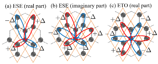
Figure 4: Schematic illustration of (a)Real part of ESE pairing, (b)Imaginary part of ESE pairing, and (c)Real part of ETO $f$-wave pairing. The dashed lines denote the unit cell. In case (c), imaginary part is negligible.

The real part is interpreted as a $d$-wave pairing and the corresponding imaginary part is $f$-wave like pairing as shown in Figs. 4(a) and (b). We have checked that ${\mathrm{Re}}[\Delta^{\mathrm{ESE}}_{A\uparrow,B\downarrow}(\bm{k},i\pi T)]={\mathrm{Re}}[\Delta^{\mathrm{ESE}}_{B\uparrow,A\downarrow}(\bm{k},i\pi T)]$ and ${\mathrm{Im}}[\Delta^{\mathrm{ESE}}_{A\uparrow,B\downarrow}(\bm{k},i\pi T)]=-{\mathrm{Im}}[\Delta^{\mathrm{ESE}}_{B\uparrow,A\downarrow}(\bm{k},i\pi T)]$ are kept. Then, $\Delta^{\mathrm{ESE}}_{A\uparrow,B\downarrow}(\bm{k},i\pi T)=\Delta^{\mathrm{ESE}}_{B\uparrow,A\downarrow}(-\bm{k},i\pi T)$ is satisfied and this relation is consistent with even-parity pairing. On the Fermi surface, the $f$-wave like imaginary component ${\mathrm{Im}}[\Delta^{\mathrm{ESE}}_{A\uparrow,B\downarrow}(\bm{k},i\pi T)]$ is larger than the $d$-wave like real one ${\mathrm{Re}}[\Delta^{\mathrm{ESE}}_{A\uparrow,B\downarrow}(\bm{k},i\pi T)]$.

Besides this ESE pairing, there is a subdominant odd-frequency pairing which is almost two orders smaller than primary ESE pairing. As shown in Fig. 5, OTE pairing is induced.

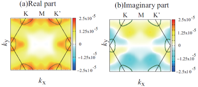
Figure 5: The subdominant OTE pairing $\Delta_{A\uparrow,B\downarrow}(\bm{k},i\pi T)$ for $\lambda_{\mathrm{SO}}/t=0.1$ and $U/t=2.75$: (a)Real part and (b)Imaginary part.

Similar to the primary ESE pairing, this induced odd-frequency gap function satisfies ${\mathrm{Re}}[\Delta^{\mathrm{OTE}}_{A\uparrow,B\downarrow}(\bm{k},i\pi T)]={\mathrm{Re}}[\Delta^{\mathrm{OTE}}_{A\uparrow,B\downarrow}(-\bm{k},i\pi T)]$ and ${\mathrm{Re}}[\Delta^{\mathrm{OTE}}_{A\uparrow,B\downarrow}(\bm{k},i\pi T)]={\mathrm{Re}}[\Delta^{\mathrm{OTE}}_{B\uparrow,A\downarrow}(\bm{k},i\pi T)]$ for real part, and ${\mathrm{Im}}[\Delta^{\mathrm{OTE}}_{A\uparrow,B\downarrow}(\bm{k},i\pi T)]=-{\mathrm{Im}}[\Delta^{\mathrm{OTE}}_{A\uparrow,B\downarrow}(-\bm{k},i\pi T)]$ and ${\mathrm{Im}}[\Delta^{\mathrm{OTE}}_{A\uparrow,B\downarrow}(\bm{k},i\pi T)]=-{\mathrm{Im}}[\Delta^{\mathrm{OTE}}_{B\uparrow,A\downarrow}(\bm{k},i\pi T)]$ for imaginary part. Then, following relation $\Delta^{\mathrm{OTE}}_{A\uparrow,B\downarrow}(\bm{k},i\pi T)=\Delta^{\mathrm{OTE}}_{B\uparrow,A\downarrow}(-\bm{k},i\pi T)$ is satisfied to be consistent with even-parity.

The reason of the generation of this subdominant OTE pairing is as follows. First, we are taking into account the Matsubara frequency dependence of the effective pairing interactions in the process of solving the $\acute{\mathrm{E}}$liahsberg equation, then the existence of the odd-frequency pairing is allowed. Second, spin-orbit coupling breaks the spin-rotational symmetry, then it causes the mixture of spin-triplet component. Since we are considering intrinsic spin-orbit coupling without momentum dependence which does not flip spin, spin-triplet component with $S_{z}=0$ is mixed as a subdominant component. The solution in Figs. 3 and 5 belongs to the E_g representation with double degeneracy. Then, the actual gap function might be a linear combination of these two solutions such as $d+id$-wave pairing.

With the increase of $\lambda_{\mathrm{SO}}$, the obtained pairing symmetry changes from ESE to ETO. As shown in Table. I, three kinds of spin state exist as a solution of the $\acute{\mathrm{E}}$liashberg equation. In the presence of $\lambda_{\mathrm{SO}}$, the degeneracy is lifted while that between $\uparrow\uparrow$ and $\downarrow\downarrow$ is kept. In the present calculation, $\uparrow\uparrow$ and $\downarrow\downarrow$ spin states are more stabilized than $\uparrow\downarrow+\downarrow\uparrow$ one.

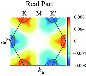
Figure 6: Real part of $\Delta_{A\uparrow,A\uparrow}(\bm{k},i\pi T)$ ETO pairing is plotted for $\lambda_{\mathrm{SO}}/t=0.5$, and $U/t=2.65$.

As shown in Fig. 6, the obtained gap function has a six-fold symmetry as a function of $\bm{k}$ and it is regarded as a $f$-wave pairing as shown in Fig. 4(c). In this case, the imaginary part of $\Delta_{A\uparrow,A\uparrow}(\bm{k},i\pi T)$ is negligible small on the Fermi surface. We have checked that $\Delta_{A\uparrow,A\uparrow}(\bm{k},i\pi T)=-\Delta_{A\uparrow,A\uparrow}(-\bm{k},i\pi T)$ and $\Delta_{A\uparrow,A\uparrow}(\bm{k},i\pi T)=\Delta_{B\uparrow,B\uparrow}(\bm{k},i\pi T)$. In this case, subdominant odd-frequency pairing never appears. This is because the presence of the spatial inversion symmetry. Since the present pair is odd-parity pairing, possible subdominant odd-frequency pairing has an OSO symmetry. On the other hand, there is no spin flipping term in the Hamiltonian. Owing to the parallel spin structure of dominant ETO pair, spin-singlet pair is prohibited.

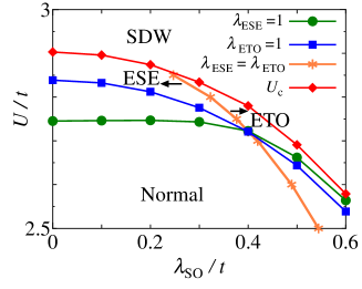
Figure 7: Phase diagram in the space of $U$ and $\lambda_{\mathrm{SO}}$ at $k_{\mathrm{B}}T/t=0.04$. $U_{\mathrm{c}}$ denotes the line above which longitudinal spin susceptibility diverges. $\lambda_{\mathrm{ESE}}=1$ ($\lambda_{\mathrm{ETO}}=1$) is a line where eigenvalue of ESE pairing (ETO $f$-wave like pairing) diverges.

In Fig. 7, we show the phase diagram obtained in this model at $k_{\mathrm{B}}T/t=0.04$. With the increase of the on-site Coulomb interaction $U$, the longitudinal spin susceptibility diverges at $U=U_{\mathrm{c}}$, and SDW phase appears for $U>U_{\mathrm{c}}$. Above the line of $\lambda_{\mathrm{ESE}}=1$ ($\lambda_{\mathrm{ETO}}=1$), ESE (ETO) pairing is stabilized. The pairing instability occurs due to the enhancement of the spin-fluctuation near the SDW phase. The line connecting crossed mark shows the line of $\lambda_{\mathrm{ESE}}=\lambda_{\mathrm{ETO}}$ in this phase diagram. At the left (right) side of this line, eigenvalue $\lambda_{\mathrm{ESE}}$ is larger (smaller) than $\lambda_{\mathrm{ETO}}$. The interesting nature is the transition from ESE pairing to ETO pairing with the increase of $\lambda_{\mathrm{SO}}$.

To understand the pairing mechanism, we show both longitudinal and transverse spin susceptibilities in the following.

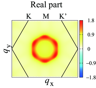
Figure 8: Real part of the longitudinal spin susceptibility $\chi^{zz}_{AA}(\bm{q},i\omega_{m}=0)$ for $\lambda_{\mathrm{SO}}/t=0.1$ and $U/t=2.75$.

The longitudinal spin susceptibility $\chi^{zz}_{AA}(\bm{q},i\omega_{m}=0)$ is shown in Fig. 8. $\chi^{zz}_{AA}(\bm{q},i\omega_{m}=0)$ becomes a real number and it has a maximum at $\bm{q}=\bm{q}_{\mathrm{c}}$, where $\bm{q}_{\mathrm{c}}$ corresponds to a momentum transfer inside Fermi pocket. By contrast to $\chi^{zz}_{AA}(\bm{q},i\omega_{m}=0)$, the longitudinal spin susceptibility $\chi^{zz}_{AB}(\bm{q},i\omega_{m}=0)$ becomes a complex number as shown in Fig. 9. It satisfies $\chi^{zz}_{AB}(\bm{q},i\omega_{m}=0)=[\chi^{zz}_{BA}(\bm{q},i\omega_{m}=0)]^{*}$. The real part of $\chi^{zz}_{AB}(\bm{q},i\omega_{m}=0)$ becomes negative. This means that effective interaction is attractive one between $A$ and $B$ sublattice. Imaginary part of $\chi^{zz}_{AB}(\bm{q},i\omega_{m}=0)$ is an odd-function of $\bm{q}$. Then, it does not contribute to the actual integral kernel of the $\acute{\mathrm{E}}$liashberg equation.

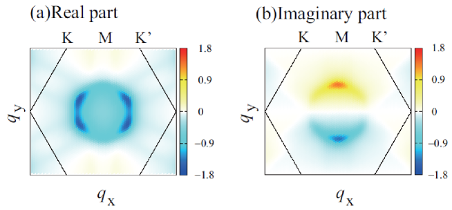
Figure 9: The longitudinal spin susceptibility $\chi^{zz}_{AB}(\bm{q},i\omega_{m}=0)$ for $\lambda_{\mathrm{SO}}/t=0.1$, and $U/t=2.75$: (a)Real part and (b)Imaginary part.

The schematic image of the pair scattering by $\bm{q}_{\mathrm{c}}$ is shown in Fig. 10. It is noted that this pair scattering occurs within each disconnected Fermi surface. In both cases with ESE and ETO pairings, there is no sign change by the pair scattering $\bm{q}_{\mathrm{c}}$. However, the reasons of the absence of sign change are different each other. Singlet and triplet channels of the effective interaction originated from longitudinal susceptibility is given by $\chi^{zz}_{\alpha\beta}(\bm{q},i\omega_{m})U^{2}/2$ and $-\chi^{zz}_{\alpha\beta}(\bm{q},i\omega_{m})U^{2}/2$, respectively. In the present ESE pairing, dominant pair is formed between $A$ and $B$ sites. In this case, $\chi^{zz}_{AB}(\bm{q},i\omega_{m})$ mainly contributes to the effective interaction. Since the real part of $\chi^{zz}_{AB}(\bm{q},i\omega_{m})$ is negative, effective interaction becomes negative, $i.e.$, attractive interaction. On the other hands, for ETO pairing, dominant pair is formed between the same sublattice sites. Then, $\chi^{zz}_{AA}(\bm{q},i\omega_{m})$ mainly contributes to the effective interaction. Though the real part of $\chi^{zz}_{AA}(\bm{q},i\omega_{m})$ is positive, effective interaction becomes negative. This is because the coefficient $-1/2$ for triplet channel gives additional sign. Then, the effective interaction for ETO channel also becomes attractive. As a result, the gap function without sign change on the Fermi surface is favorable as shown in Fig. 10.

Figure 10: Schematic illustrations of the momentum transfer by the pair scattering at $\bm{q}=\bm{q}_{\mathrm{c}}$. (a)Imaginary part of the energy gap function for ESE pairing has a sign change by pair scattering. (b)Enlarged view of (a). (c)Read part of the energy gap function for ETO $f$-wave pairing does not have a sign change by pair scattering. (d)Enlarged view of (c).

In order to clarify how spin fluctuation is influenced by $\lambda_{\mathrm{SO}}$, we study spin susceptibility at $\bm{q}=\bm{q}_{\mathrm{c}}$ and $\bm{q}=0$ as a function of $\lambda_{\mathrm{SO}}$. At $\lambda_{\mathrm{SO}}=0$, $2\chi^{zz}_{\alpha\beta}=\chi^{+-}_{\alpha\beta}$ is satisfied due to the spin- rotational symmetry. However, this relation is broken in the presence of $\lambda_{\mathrm{SO}}$.

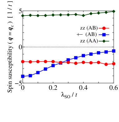
Figure 11: Longitudinal and transverse spin susceptibilities are plotted as a function of $\lambda_{\mathrm{SO}}$ for $U=0.98U_{\mathrm{c}}$ and $\bm{q}=\bm{q}_{\mathrm{c}}$. $zz$ ($\alpha\beta$) and $+-$($\alpha\beta$) denote longitudinal spin susceptibility $\mathrm{Re}[\chi^{zz}_{\alpha\beta}(\bm{q},i\omega_{m}=0)]$ and transverse spin susceptibility $\mathrm{Re}[\chi^{+-}_{\alpha\beta}(\bm{q},i\omega_{m}=0)]$.

First, we show the case with $\bm{q}=\bm{q}_{\mathrm{c}}$ (Fig. 11). The magnitude of $\mathrm{Re}[\chi^{+-}_{AB}(\bm{q}=\bm{q}_{\mathrm{c}},i\omega_{m}=0)]$ is greatly suppressed with the increase of $\lambda_{\mathrm{SO}}$. On the other hand, the magnitude of $\mathrm{Re}[\chi^{zz}_{AA}(\bm{q}=\bm{q}_{\mathrm{c}},i\omega_{m}=0)]$ and $\mathrm{Re}[\chi^{zz}_{AB}(\bm{q}=\bm{q}_{\mathrm{c}},i\omega_{m}=0)]$ are little bit enhanced.

Figure 12: Longitudinal and transverse spin susceptibilities are plotted as a function of $\lambda_{\mathrm{SO}}$ for $U=0.98U_{\mathrm{c}}$ and $\bm{q}=0$. $zz$ ($\alpha\beta$) and $+-$($\alpha\beta$) denote longitudinal spin susceptibility $\chi^{zz}_{\alpha\beta}(\bm{q},i\omega_{m}=0)$ and transverse spin suceptibilitibility $\chi^{+-}_{\alpha\beta}(\bm{q},i\omega_{m}=0)$.

Next, we show the case with $\bm{q}=0$ (Fig. 12). The magnitude of $\chi^{+-}_{AB}(\bm{q}=0,i\omega_{m}=0)$ is suppressed with the increase of $\lambda_{\mathrm{SO}}$ similar to the case of $\bm{q}=\bm{q}_{\mathrm{c}}$. On the other hand, the magnitude of $\chi^{zz}_{AA}(\bm{q}=0,i\omega_{m}=0)$ and $\chi^{zz}_{AB}(\bm{q}=\bm{q}_{\mathrm{c}},i\omega_{m}=0)$ are enhanced. The degree of enhancement of $\chi^{zz}_{AA}(\bm{q}=0,i\omega_{m}=0)$ is greater than that of $\chi^{zz}_{AB}(\bm{q}=0,i\omega_{m}=0)$.

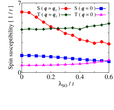
Figure 13: The absolute value of spin susceptibilities are plotted as a function of $\lambda_{\mathrm{SO}}$ for $U=0.98U_{\mathrm{c}}$ with $\bm{q}=\bm{q}_{\mathrm{c}}$ and $\bm{q}=0$. $S(\bm{q}=\bm{q}_{\mathrm{c}})=|\mathrm{Re}[\chi^{zz}_{AB}(\bm{q}_{\mathrm{c}},i\omega_{m}=0)+\chi^{+-}_{AB}(\bm{q}_{\mathrm{c}},i\omega_{m}=0)]|$, $S(\bm{q}=0)=|\mathrm{Re}[\chi^{zz}_{AB}(0,i\omega_{m}=0)+\chi^{+-}_{AB}(0,i\omega_{m}=0)]|$, $T(\bm{q}=\bm{q}_{\mathrm{c}})=|\mathrm{Re}[\chi^{zz}_{AA}(\bm{q}_{\mathrm{c}},i\omega_{m}=0)]|$, and $T(\bm{q}=0)=|\mathrm{Re}[\chi^{zz}_{AA}(0,i\omega_{m}=0)]|.$

In Fig. 13, to see the strength of pairing interaction, we plot

$$S(\bm{q}=\bm{q}_{\mathrm{c}}) =|\mathrm{Re}[\chi^{zz}_{AB}(\bm{q}_{\mathrm{c}},i\omega_{m}=0)+\chi^{+-}_{AB}(\bm{q}_{\mathrm{c}},i\omega_{m}=0)]|,$$ (36)

$$S(\bm{q}=0) =|\mathrm{Re}[\chi^{zz}_{AB}(0,i\omega_{m}=0)+\chi^{+-}_{AB}(0,i\omega_{m}=0)]|,$$ (37)

$$T(\bm{q}=\bm{q}_{\mathrm{c}}) =|\mathrm{Re}[\chi^{zz}_{AA}(\bm{q}_{\mathrm{c}},i\omega_{m}=0)]|,$$ (38)

$$T(\bm{q}=0) =|\mathrm{Re}[\chi^{zz}_{AA}(0,i\omega_{m}=0)]|.$$ (39)

Here, $S(\bm{q})$ and $T(\bm{q})$ express the spin fluctuation which contributes to ESE pairing and ETO pairing, respectively. As seen in Fig. 13, the magnitude of $S(\bm{q}=\bm{q}_{\mathrm{c}})$ is strongly suppressed by spin-orbit coupling $\lambda_{\mathrm{SO}}$. The magnitude of $S(\bm{q}=0)$ is also reduced. This is the reason that ESE pairing becomes destabilized with $\lambda_{\mathrm{SO}}$. On the other hand, $T(\bm{q}=\bm{q}_{\mathrm{c}})$ and $T(\bm{q}=0)$ are enhanced with $\lambda_{\mathrm{SO}}$. This is the reason why ETO pairing becomes dominant with $\lambda_{\mathrm{SO}}$.

Summarizing these results, ESE pairing is induced by transverse spin fluctuation at $\bm{q}=\bm{q}_{\mathrm{c}}$. On the other hand, ETO $f$-wave pairing is supported by longitudinal spin fluctuation at $\bm{q}=\bm{q}_{\mathrm{c}}$ and $\bm{q}=0$. Since the transverse spin fluctuation is strongly suppressed by spin-orbit coupling, ETO $f$-wave pairing becomes dominant for large $\lambda_{\mathrm{SO}}$.

4 Summary

In this paper, we have studied possible pairing symmetries of a doped Kane-Mele model on the honeycomb lattice with on-site Coulomb interaction. We have clarified the pairing instability of Cooper pair by the linearized $\acute{\mathrm{E}}$liashberg equation within RPA. When the magnitude of the spin-orbit coupling is weak, ESE pairing becomes dominant one. Since Cooper pair is formed between $A$ and $B$ sites in this pairing, it has a complicated momentum dependence. In our choice of the gauge, real part has a $d$-wave symmetry while imaginary part has a $f$-wave like symmetry. This $f$-wave like pairing does not contradict even-parity pairing because it has a sign change with the exchange of the index $A$ and $B$. At the same time, OTE pairing with $S_{z}=0$ also mixes as a subdominant component of a solution of the $\acute{\mathrm{E}}$liashberg equation. It is triggered by the intrinsic spin-orbit coupling which does not flip the spin. By contrast to ESE dominant case, odd-frequency subdominant pair never appears since spin-triplet $f$-wave pair is composed of two electrons with equal spin. With the increase of the magnitude of spin-orbit coupling, we have clarified that the spin-triplet $f$-wave pairing becomes dominant. This is because the transverse spin susceptibility is suppressed by spin-orbit coupling and the resulting effective interaction for ESE channel is weakened.

In this paper, we have focused on the pairing mechanism of doped Kane-Mele model and found the instability of unconventional superconductivity. Nowadays, it is known that both even and odd-parity pairings discussed in this paper have surface Andreev bound states (SABS) which are protected by topological invariants [52, 53]. It is interesting to calculate SABS and tunneling spectroscopy via Andreev bound state [54, 55, 56] in order to distinguish spin-triplet odd-parity pairing from spin-singlet even-parity one. Especially charge transport in diffusive normal metal / spin-triplet odd-parity superconductor is interesting since we have obtained anomalous proximity effect by odd-frequency pairing and Majorana fermion in diffusive normal metal / spin-triplet $p$-wave superconductor junctions [57, 58, 59, 60].

- [1] M. Sigrist and K. Ueda: Rev. Mod. Phys. 63 (1991) 239.
- [2] D. J. Van Harlingen: Rev. Mod. Phys. 67 (1995) 515.
- [3] T. Moriya and K. Ueda: Advances in Physics 49 (2000) 555.
- [4] P. A. Lee, N. Nagaosa, and X.-G. Wen: Rev. Mod. Phys. 78 (2006) 17.
- [5] M. Ogata and H. Fukuyama: Reports on Progress in Physics 71 (2008) 036501.
- [6] C. C. Tsuei and J. R. Kirtley: Rev. Mod. Phys. 72 (2000) 969.
- [7] S. Kashiwaya and Y. Tanaka: Rep. Prog. Phys. 63 (2000) 1641.
- [8] A. J. Leggett: Rev. Mod. Phys. 47 (1975) 331.
- [9] Y. Maeno, S. Kittaka, T. Nomura, S. Yonezawa, and K. Ishida: Journal of the Physical Society of Japan 81 (2012) 011009.
- [10] K. Kuroki, R. Arita, and H. Aoki: Phys. Rev. B 63 (2001) 094509.
- [11] Y. Tanaka and K. Kuroki: Phys. Rev. B 70 (2004) 060502.
- [12] K. Kuroki, Y. Tanaka, and R. Arita: Phys. Rev. Lett. 93 (2004) 077001.
- [13] H. Ikeda, Y. Nisikawa, and K. Yamada: Journal of the Physical Society of Japan 73 (2004) 17.
- [14] Y. Tanaka, Y. Yanase, and M. Ogata: Journal of the Physical Society of Japan 73 (2004) 319.
- [15] Y. Nisikawa, H. Ikeda, and K. Yamada: Journal of the Physical Society of Japan 73 (2004) 1127.
- [16] K. Kuroki and Y. Tanaka: Journal of the Physical Society of Japan 74 (2005) 1694.
- [17] D. Jerome, A. Mazaud, M. Ribault, and K. Bechgaard: J. Physique Lett. 41 (1980) 95.
- [18] J. C. Nickel, R. Duprat, C. Bourbonnais, and N. Dupuis: Phys. Rev. Lett. 95 (2005) 247001.
- [19] Y. Fuseya and Y. Suzumura: Journal of the Physical Society of Japan 74 (2005) 1263.
- [20] H. Aizawa, K. Kuroki, and Y. Tanaka: Phys. Rev. B 77 (2008) 144513.
- [21] H. Aizawa, K. Kuroki, T. Yokoyama, and Y. Tanaka: Phys. Rev. Lett. 102 (2009) 016403.
- [22] H. Aizawa, K. Kuroki, and Y. Tanaka: Journal of the Physical Society of Japan 78 (2009) 124711.
- [23] K. Takada, H. Sakurai, E. Takayama-Muromachi, F. Izumi, and R. Dilanian: Nature 422 (2003) 53.
- [24] K. Kuroki, Y. Tanaka, and R. Arita: Phys. Rev. B 71 (2005) 024506.
- [25] Y. Yanase, M. Mochizuki, and M. Ogata: Journal of the Physical Society of Japan 74 (2005) 430.
- [26] Y. Yanase, M. Mochizuki, and M. Ogata: Journal of the Physical Society of Japan 74 (2005) 2568.
- [27] I. I. Mazin and M. D. Johannes: Nature Physics 1 (2005) 91.
- [28] M. Mochizuki, Y. Yanase, and M. Ogata: Phys. Rev. Lett. 94 (2005) 147005.
- [29] K. Yada and H. Kontani: Journal of the Physical Society of Japan 75 (2006) 033705.
- [30] K. Yada and H. Kontani: Phys. Rev. B 77 (2008) 184521.
- [31] M. Sato, Y. Kobayashi, and T. Moyoshi: Physica C: Superconductivity 470 (2010) S673 .
- [32] J. Sauls: Advances in Physics 43 (1994) 113.
- [33] Y. Tsutsumi, M. Ishikawa, T. Kawakami, T. Mizushima, M. Sato, M. Ichioka, and K. Machida: Journal of the Physical Society of Japan 82 (2013) 113707.
- [34] J. Goryo, M. H. Fischer, and M. Sigrist: Phys. Rev. B 86 (2012) 100507.
- [35] W.-S. Wang, Y. Yang, and Q.-H. Wang: Phys. Rev. B 90 (2014) 094514.
- [36] W.-C. Lee, C. Wu, and S. Das Sarma: Phys. Rev. A 82 (2010) 053611.
- [37] C. Honerkamp: Phys. Rev. Lett. 100 (2008) 146404.
- [38] M. L. Kiesel, C. Platt, W. Hanke, D. A. Abanin, and R. Thomale: Phys. Rev. B 86 (2012) 020507.
- [39] M. L. Kiesel and R. Thomale: Phys. Rev. B 86 (2012) 121105.
- [40] M. L. Kiesel, C. Platt, and R. Thomale: Phys. Rev. Lett. 110 (2013) 126405.
- [41] R. Nandkishore, R. Thomale, and A. V. Chubukov: Phys. Rev. B 89 (2014) 144501.
- [42] L. Zhang, F. Yang, and Y. Yao: Scientific Reports 5 (2015) 8203.
- [43] K. S. Novoselov, A. K. Geim, S. V. Morozov, D. Jiang, Y. Zhang, S. V. Dubonos, I. V. Grigorieva, and A. A. Firsov: Science 306 (2004) 666.
- [44] J. T. Ye, Y. J. Zhang, R. Akashi, M. S. Bahramy, R. Arita, and Y. Iwasa: Science 50 (2012) 14916.
- [45] R. Nandkishore, L. S. Levitov, and A. V. Chubukov: Nature Physics 8 (2012) 158.
- [46] L. Chen, B. Feng, and K. Wu: Applied Physics Letters 102 (2013).
- [47] N. F. Q. Yuan, K. F. Mak, and K. T. Law: Phys. Rev. Lett. 113 (2014) 097001.
- [48] A. M. Black-Schaffer and C. Honerkamp: Journal of Physics: Condensed Matter 26 (2014) 423201.
- [49] G. Baskaran: arXiv:1309.2242 .
- [50] C. L. Kane and E. J. Mele: Phys. Rev. Lett. 95 (2005) 146802.
- [51] C. L. Kane and E. J. Mele: Phys. Rev. Lett. 95 (2005) 226801.
- [52] M.Sato, Y.Tanaka, K.Yada, and T.Yokoyama: Phys. Rev. B 83 (2011) 224511.
- [53] Y. Tanaka, M. Sato, and N. Nagaosa: J. Phys. Soc. Jpn. 81 (2012) 011013.
- [54] Y. Tanaka and S. Kashiwaya: Phys. Rev. Lett. 74 (1995) 3451.
- [55] Y. Tanuma, K. Kuroki, Y. Tanaka, and S. Kashiwaya: Phys. Rev. B 64 (2001) 214510.
- [56] Y. Tanuma, K. Kuroki, Y. Tanaka, R. Arita, S. Kashiwaya, and H. Aoki: Phys. Rev. B 66 (2002) 094507.
- [57] Y. Tanaka and S. Kashiwaya: Phys. Rev. B 70 (2004) 012507.
- [58] Y. Tanaka, S. Kashiwaya, and T. Yokoyama: Phys. Rev. B 71 (2005) 094513.
- [59] Y. Tanaka and A. A. Golubov: Phys. Rev. Lett. 98 (2007) 037003.
- [60] Y. Asano and Y. Tanaka: Phys. Rev. B 87 (2013) 104513.