Abstract

Minkowski space, namely $\mathbb{R}^{3}$ endowed with the quadradic form $-\mathrm{d}t^{2}+\mathrm{d}x^{2}+\mathrm{d}y^{2}$, is the local model of 3 dimensionnal flat spacetimes. Recent progress in the description of globally hyperbolic flat spacetimes showed strong link between Lorentzian geometry and Teichmüller space. We notice that Lorentzian generalisations of conical singularities are useful for the endeavours of descripting flat spacetimes, creating stronger links with hyperbolic geometry and compactifying spacetimes. In particular massive particles and extreme BTZ singular lines arise naturally. This paper is three-fold. First, prove background properties which will be useful for future work. Second generalise fundamental theorems of the theory of globally hyperbolic flat spacetimes. Third, defining BTZ-extension and proving it preserves Cauchy-maximality and Cauchy-completeness.

all

Laboratoire de Mathématiques d’Avignon
Université d’Avignon et des pays du Vaucluse

Léo Brunswic
March 12, 2024

1 Introduction

1.1 Context and motivations

The main interest of our study are singular flat globally hyperbolic Cauchy-complete spacetimes. This paper is part of a longer-term objective : construct correspondances between spaces of hyperbolic surfaces, singular spacetimes and singular Euclidean surfaces. A central point which underlies this entire paper as well as a following to come is as follows. Starting from a compact surface $\Sigma$ with a finite set $S$ of marked points, the Teichmüller space of $(\Sigma,S)$ is the set of complete hyperbolic metric on $\Sigma\setminus S$ up to isometry. The universal cover of a point of the Teichmüller space is the Poincaré disc $\mathbb{H}^{2}$ which embbeds in the 3-dimensional Minkowki space, denoted by $\mathbb{E}^{1,2}$. Namely, Minkoswki space is $\mathbb{R}^{3}$ endowed with the undefinite quadratic form $-\mathrm{d}t^{2}+\mathrm{d}x^{2}+\mathrm{d}y^{2}$ where $(t,x,y)$ are the carthesian coordinates of $\mathbb{R}^{3}$ and the hyperbolic plane embbeds as the quadric $\{-t^{2}+x^{2}+y^{2}=-1,t>0\}$. It is in fact in the cone $C=\{t>0,-t^{2}+x^{2}+y^{2}<0\}$ which direct isometry group is exactly the group of isometry of the Poincaré disc : $\mathrm{SO}_{0}(1,2)$. A point of Teichmüller space can then be described as a representation of the fundamental group $\pi_{1}\left(\Sigma\setminus S\right)$ in $\mathrm{SO}_{0}(1,2)$ which image is a lattice $\Gamma$. If the set of marked points is trivial, $S=\emptyset$, then the lattice $\Gamma$ is uniform. The hyperbolic surface $\mathbb{H}^{2}/\Gamma$ embeds into $C/\Gamma$ giving our first non trivial examples of flat globally hyperbolic Cauchy-compact spacetimes. If on the contrary, the set of marked point is not trivial, $S\neq\emptyset$, then the lattice $\Gamma$ contains parabolic isometries each of which fixes point-wise a null ray on the boundary of the cone $C$. The cusp of the hyperbolic metric on $\Sigma\setminus S$ correspond bijectively to the equivalence classes of these null rays under the action of $\Gamma$. More generally, take a discrete subgroup $\Gamma$ of $\mathrm{SO}_{0}(1,2)$. The group $\Gamma$ may have an elliptic isometries i.e. a torsion part. Therefore, on the one hand $\mathbb{H}^{2}/\Gamma$ is a complete hyperbolic surface with conical singularities. On the other hand, $C/\Gamma$ is a flat spacetime with a Lorentzian analogue of conical singularities : massive particles. This spacetime admits a connected sub-surface which intersects exactly once every rays from the origin in the cone $C$. Furthermore, this sub-surface is naturally endowed with a riemannian metric with respect to which it is complete. As an example, consider the modular group $\Gamma=\mathrm{PSL}(2,\mathbb{Z})$. A fundamental domain of the action of $\mathrm{PSL}(2,\mathbb{Z})$ on $\mathbb{H}^{2}$ is decomposed into two triangles isometric to the same ideal hyperbolic triangle $T$ of angles $\frac{\pi}{2}$ and $\frac{\pi}{3}$ . The surface $\mathbb{H}^{2}/\Gamma$ is then obtained by gluing edge to edge these two triangles (see [Rat] for more details about the modular group). The suspension of the hyperbolic triangle $T$ is $\mathrm{Susp}(T)=\mathbb{R}_{+}^{*}\times T$ with the metric $-\mathrm{d}t^{2}+t^{2}\mathrm{d}s_{T}^{2}$. It can be realised as a cone of triangular basis in Minkoswki space as shown on figure 1.a. An edge of the triangulation of $\mathbb{H}^{2}/\Gamma$ corresponds to a face of one of the two suspensions, then the suspensions can be glued together face to face accordingly. In this way we obtain this way a flat spacetime but the same way the vertices of the triangulation give rise to conical singularities, the vertical edges will give rise to singular lines in our spacetime. There are three singular lines we can put in two categories following the classification of Barbot, Bonsante and Schlenker [BBS11, BBS14].

• Two massive particles going through the conical singularities of $\mathbb{H}^{2}/\Gamma$. The corresponding vertical edges are endowed with a negative-definite semi-riemannian metric.

• One extreme BTZ-line toward which the cusp of $\mathbb{H}^{2}/\Gamma$ seems to tend like in figure 1.b. The corresponding vertical edge is endowed with a null semi-riemannian metric.

The spacetime $C/\Gamma$ can be recovered by taking the complement of the extreme BTZ-line. Still, we constructed something more which satisfies two interesting properties.

• Take a horizontal plane in Minkoswki space above the origin. It intersects $\mathrm{Susp}(T)$ along a Euclidean triangle. The gluing of the suspensions induces a gluing of the corresponding Euclidean triangles. We end up with a polyhedral surface which intersects exactly once every rays from the origin : our singular spacetime with extreme BTZ-line have a polyhedral Cauchy-surface.

• This polyhedral surface is compact. Therefore, the spacetime with extreme BTZ-line is Cauchy-compact when $C/\Gamma$ is merely Cauchy-complete.

a) A fundamental domain of $\mathrm{PSL}(2,\mathbb{Z})$ in $\mathbb{H}^{2}$.	b) An embedding in $\mathbb{E}^{1,2}$ and its suspension.

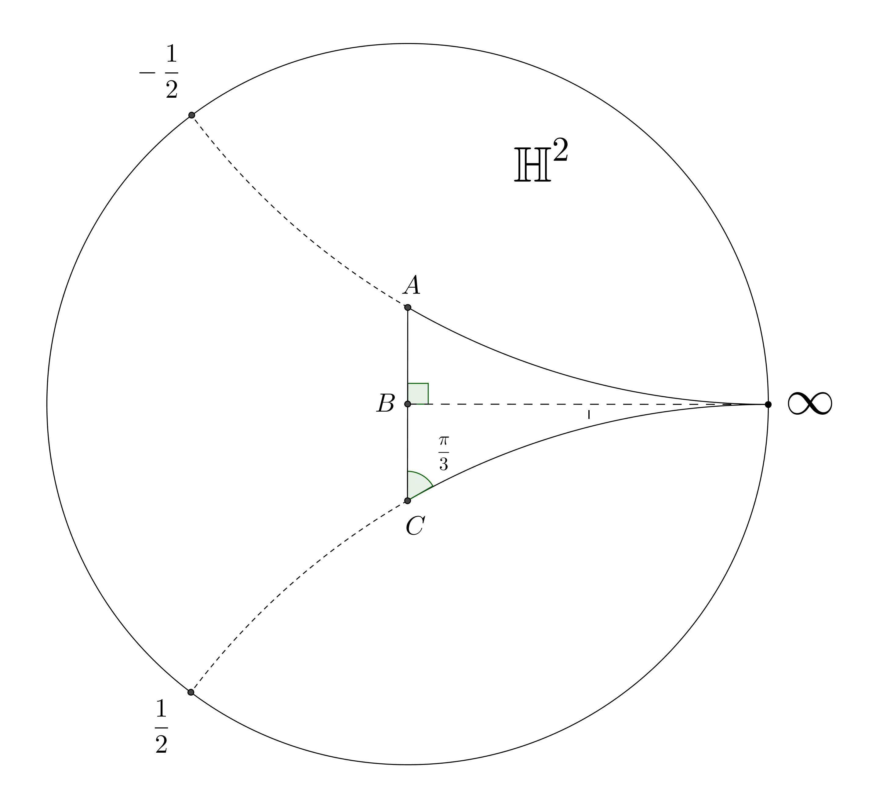
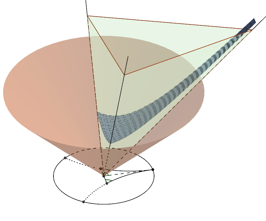
Figure 1: Fundamental domain of the modular group and its suspension.

The fundamental domain of the modular group is represented on the left in the Poincaré disc. The triangles $[AB\infty]$ and $[CB\infty]$ are symetric with respect to the line $(B\infty)$. The modular group sends the edge $[BC]$ on the edge $[BA]$ via an elliptic isometry of angle $\pi$. It sends the edge $[A\infty]$ to $[C\infty]$ via a parabolic isometry of center $\infty$. On the right is depicted the natural embedding of this fundamental domain in Minkoswki space in deep blue. The light blue cone of triangular basis is its suspension. The null cone of Minkoswki space is in red. The stereograpic projection of the Poincaré disc is depicted on the horizontal plane $\{t=0\}$ .

This paper is devoted to the description of the process by which BTZ-lines are added and how it interacts with global properties of the spacetime : global hyperbolicity, Cauchy-completeness and Cauchy-maximality. Since a general theory of such singular spacetimes is lacking, part of the paper is devoted to background properties. A following paper will be devoted to the construction of singular Euclidean surfaces in singular spacetimes as well as a correspondance between hyperbolic, Minkowskian and Euclidean objects. Some compactification properties will also be dealt with.

1.2 Structure of the paper and goals

The paper gives the definition of singular spacetimes as well as Cauchy-something properties and develop some basic properties in section 1.5. Its primary objectives are the following

1. Define a notion of BTZ-extension and prove a maximal BTZ-extension existence and uniqueness theorem. This is Theorem II in Section 3.

2. Prove that Cauchy-completeness and Cauchy-maximality are compatible with BTZ-extensions. This is Theorem III in section 4.

Some secondary objectives are needed both to complete the picture and to the proofs of the main theorems.

1. Prove local rigidity property which is an equivalent of local unicity of solution of Einstein equations in our context. This ensure we have a maximal Cauchy-extension existence and uniqueness theorem, much alike the one of Choquet-Bruhat-Geroch, stated in Section 2.2. The local rigidity is done in Section 1.4.3.

2. Prove the existence of a smooth Cauchy-surface in a globally hyperbolic singular spacetime. Theorem I proves it in Section 2.3.

3. Show that in a Cauchy-maximal spacetime, BTZ-singular lines are complete in the future and posess standard neighborhoods. A proof is given in Section 2.2

1.3 Global properties of regular spacetimes

1.3.1 $(G,X)$-structures

$(G,X)$-structures are used in the preliminary of the present work and may need some reminders. Let $X$ be a topological space and $G\subset\mathrm{Homeo}(X)$ be a group of homeomorphism. The couple $(G,X)$ is an analytical structure if two elements of $G$ agreeing on a non trivial open subset of $X$ are equal. Given $(G,X)$ an analytical structure and $M$ a Hausdorff topological space, a $(G,X)$-structure on $M$ is the data of an atlas $(\mathcal{U}_{i},\varphi_{i})_{i\in I}$ where $\varphi_{i}:\mathcal{U}_{i}\rightarrow\mathcal{V}_{i}\subset X$ are homeomorphisms such that for every $i,j\in I,$ there exists an element $g\in G$ agreeing with $\varphi_{j}\circ\varphi_{i}^{-1}$ on $\mathcal{V}_{i}\cap\phi_{i}(\mathcal{U}_{j}\cap\mathcal{U}_{i})$. A manifold together with a $(G,X)$-structure is a $(G,X)$-manifold. The morphisms $M\rightarrow M^{\prime}$ of $(G,X)$-manifolds are the functions $f:M\rightarrow M^{\prime}$ such that for all couples of charts $(\mathcal{U},\varphi)$ and $(\mathcal{U}^{\prime},\varphi^{\prime})$ of $M$ and $M^{\prime}$ respectively, $\varphi^{\prime}\circ f\circ\varphi^{-1}:\varphi(\mathcal{U}\cap f^{-1}(\mathcal{U}^{\prime}))\rightarrow\varphi^{\prime}(\mathcal{U}^{\prime})$ is the restriction of an element of $G$. Given a local homeomorphism $f:M\rightarrow N$ between differentiable manifolds, for every $(G,X)$-structure on $N$, there exists a unique $(G,X)$-structure on $M$ such that $f$ is a $(G,X)$-morphism. Writing $\widetilde{M}$ the universal covering of a manifold $M$ and $\pi_{1}(M)$ its fundamental group, there exists a unique $(G,X)$-structure on $\widetilde{M}$ such that the projection $\pi:\widetilde{M}\rightarrow M$ is a $(G,X)$-morphism.

Proposition 1.1 (Fundamental property of $(G,X)$-structures).

Let $M$ be a $(G,X)$-manifold. There exists a map $\mathcal{D}:\widetilde{M}\rightarrow X$ called the developping map, unique up to composition by an element of $G$ ; and a morphism $\rho:\pi_{1}(M)\rightarrow G$, unique up to conjugation by an element of $G$ such that $\mathcal{D}$ is a $\rho$-equivariant $(G,X)$-morphism.

Actually, the analyticity of the $(G,X)$-structure ensure that every $(G,X)$-morphism $\widetilde{M}\rightarrow X$ is a developping map.

1.3.2 Minkowski space

The only analytical structure we shall deal with is minkowskian.

Definition 1.2 (Minkowski space).

Let $\mathbb{E}^{1,2}=\left(\mathbb{R}^{3},q\right)$ be the Minkowski space of dimension 3 where $q$ is the bilinear form $-\mathrm{d}t^{2}+\mathrm{d}x^{2}+\mathrm{d}y^{2}$ and $t,x,y$ denote respectively the carthesian coordinates of $\mathbb{R}^{3}$. A non zero vector $u\in\mathbb{E}^{1,2}\setminus\{0\}$ is spacelike, lightlike or timelike whether $q(u,u)$ is positive, zero or negative. A vector is causal if it is timelike or lightlike. The set of non zero causal vectors is the union of two convex cones, the one in which $t$ is positive is the future causal cone and the other is the past causal cone. A continuous piecewise differentiable curve in $\mathbb{E}^{1,2}$ is future causal (resp. chronological) if at all points its tangent vectors are future causal (resp. timelike). The causal (resp. chronological) future of a point $p\in\mathbb{E}^{1,2}$ is the set of points $q$ such that there exists a future causal (resp. chronological) curve from $p$ to $q$ ; it is written $J^{+}(p)$ (resp. $I^{+}(p)$).

Consider a point $p\in\mathbb{E}^{1,2}$, we have

• $I^{+}(p)=\{q\in\mathbb{E}^{1,2}\leavevmode\nobreak\ |\leavevmode\nobreak\ q-p\text{ future timelike}\}$

• $J^{+}(p)=\{q\in\mathbb{E}^{1,2}\leavevmode\nobreak\ |\leavevmode\nobreak\ q-p\text{ future causal or zero}\}$

The causality defines two order relations on $\mathbb{E}^{1,2}$, the causal relation $<$ and the chronological relation $\ll$. More precisely, $x<y$ iff $y\in J^{+}(x)\setminus\{x\}$ and $x\ll y$ iff $y\in I^{+}(x)$. One can then give the most general definition of causal curve. A causal (resp. chronological) curve is a continous curve in $\mathbb{E}^{1,2}$ increasing for the causal (resp. chronological) order. A causal (resp. chronological) curve is inextendible if every causal (resp. chronological) curve containing it is equal. The causal order relation is often called a causal orientation.

Proposition 1.3.

The group $\mathrm{Isom}(\mathbb{E}^{1,2})$ of affine isometries of $\mathbb{E}^{1,2}$ preserving the orientation and preserving the causal order is the identity component of the group of affine isometries of $\mathbb{E}^{1,2}$. Its linear part $\mathrm{SO}_{0}(1,2)$ is the identity component of $\mathrm{SO}(1,2)$.

A linear isometry either is the identity or possesses exactly one fixed direction. It is elliptic (resp. parabolic, resp. hyperbolic) if its line of fixed points is timelike (resp. lightlike, resp. spacelike). Any $(\mathrm{Isom}(\mathbb{E}^{1,2}),\mathbb{E}^{1,2})$-manifold, is naturally causally oriented. Since there are no ambiguity on the group, we will refer to $\mathbb{E}^{1,2}$-manifold

1.3.3 Globally hyperbolic regular spacetimes

A characterisation of $\mathbb{E}^{1,2}$-manifolds, to be reasonable, needs some assumptions.

Definition 1.4.

A subset $P\subset M$ of a spacetime $M$ is acausal if any causal curve intersects $P$ at most once.

Definition 1.5 (Globally hyperbolic $\mathbb{E}^{1,2}$-structure).

A $\mathbb{E}^{1,2}$-manifold $M$ is globally hyperbolic if there exists a topological surface $\Sigma$ in $M$ such that every inextendible causal curve in $M$ intersects $\Sigma$ exactly once. In particular $\Sigma$ is acausal. Such a surface is called a Cauchy-surface.

Definition 1.6 (Cauchy-embedding).

A Cauchy-embedding $f:M\rightarrow N$ between two globally hyperbolic manifolds is an isometric embedding sending a Cauchy-surface (hence every) on a Cauchy-surface. We say that $N$ is a Cauchy-extension of $M$.

A piecewise smooth surface is called spacelike if every tangent vector is spacelike. Such a surface is endowed with a metric space structure induced by the ambiant $\mathbb{E}^{1,2}$-structure. If this metric space is metrically complete, the surface is said complete.

Definition 1.7.

A spacetime admitting a metrically complete piecewise smooth and spacelike Cauchy-surface is called Cauchy-complete.

There is a confusion not to make between Cauchy-complete in this meaning and ”metrically complete” which is sometimes refered to by ”Cauchy complete” : here, the spacetime is not even a metric space. Geroch and Choquet-Bruhat [CBG69] proved the existence and uniqueness of the maximal Cauchy-extension of globally hyperbolic Lorentz manifolds satisfying certain Einstein equations (see [Rin09] for a more modern approach). Our special case correspond to vacuum solutions of Einstein equations. There thus exists a unique maximal Cauchy-extension of a given spacetime. Mess [Mes07] and then Bonsante, Benedetti, Barbot and others [Bar05], [ABB⁺07], constructed a characterisation of maximal Cauchy-complete globally hyperbolic $\mathbb{E}^{1,n}$-manifolds for all $n\in\mathbb{N}^{*}$. This caracterisation is based on the holonomy. We are only concerned in the $n=2$ case.

1.4 Massive particle and BTZ white-hole

1.4.1 Definition and causality

Lorentzian analogue in dimension 3 of conical singularities have been classified in [BBS11]. We are only interested in two specific types we describe below : massive particles and BTZ lines. Massive particles are the most direct Lorentzian analogues of conical singularities. A Euclidean conical singularity can be constructed by quotienting the Euclidean plane by a finite rotation group. The conical angle is then $2\pi/k$ for some $k\in\mathbb{N}^{*}$. The same way, one can construct examples of massive particles by quotienting $\mathbb{E}^{1,2}$ by some finite group of elliptic isometries. The general definitions are as follow. Take the universal covering of the complement of a point in the Euclidean plane. It is isometric to $\mathbb{E}_{\infty}^{2}:=(\mathbb{R}_{+}^{*}\times\mathbb{R},\mathrm{d}r^{2}+r^{2}\mathrm{d}\theta^{2})$. The translation $(r,\theta)\mapsto(r,\theta+\theta_{0})$ are isometries, one can then quotient out $\mathbb{E}^{2}_{\infty}$ by some discrete translation group $\theta_{0}\mathbb{Z}$. The quotient is an annulus $\mathbb{R}_{+}^{*}\times\mathbb{R}/2\pi\mathbb{Z}$ with the metric $\mathrm{d}r^{2}+\theta_{0}r^{2}\mathrm{d}\theta^{2}$ which can be completed by adding one point. The completion is then homeomorphic to $\mathbb{R}^{2}$ but the total angle around the origin is $\theta_{0}$ instead of $2\pi$. Define the model of a massive particle of angle $\alpha$ by the product of a conical singularity of conical angle $\alpha$ by $(\mathbb{R},-\mathrm{d}t^{2})$.

Definition 1.8 (Conical singularity).

Let $\alpha\in\mathbb{R}_{+}^{*}$. The singular plane of conical angle $\alpha$, written $\mathbb{E}^{2}_{\alpha}$, is $\mathbb{R}^{2}$ equipped with the metric expressed in polar coordinates

$$\mathrm{d}r^{2}+\frac{\alpha}{2\pi}r^{2}\mathrm{d}\theta^{2}.$$

The metric is well defined and flat everywhere but at $0$ which is a singular point. The space can be seen as the metric completion of the complement of the singular point. The name comes from the fact the metric of a cone in $\mathbb{E}^{3}$ can be written this way in a suitable coordinate system. While Euclidean cones have a conical angle less than $2\pi$, a spacelike revolution cone of timelike axis in Minkowski space is isometric to $\mathbb{E}^{2}_{\alpha}$ with $\alpha$ greater that $2\pi$. We insist on the fact that the parameter $\alpha$ is an arbitrary positive real number.

Definition 1.9 (Massive particles model spaces).

Let $\alpha$ be a positive real number. We define :

$$\mathbb{E}^{1,2}_{\alpha}:=(\mathbb{R}\times\mathbb{E}^{2}_{\alpha},\mathrm{d}s^{2})\text{ with }\mathrm{d}s^{2}=-\mathrm{d}t^{2}+\mathrm{d}r^{2}+\frac{\alpha}{2\pi}r^{2}\mathrm{d}\theta^{2}$$

where $t$ is the first coordinate of the product and $(r,\theta)$ the polar coordinates of $\mathbb{R}^{2}$ (in particular $\theta\in\mathbb{R}/2\pi\mathbb{Z}$). The complement of the singular line $\mathrm{Sing}(\mathbb{E}^{1,2}_{\alpha}):=\{r=0\}$ is a spacetime called the regular locus and denoted by $Reg(\mathbb{E}^{1,2}_{\alpha})$. For $p\in\mathrm{Sing}(\mathbb{E}^{1,2}_{\alpha})$, we write $]p,+\infty[$ (resp. $[p,+\infty[$) for the open (resp. closed) future singular ray from $p$. We will also use analogue notation of the past singular ray from $p$.

Start from a massive particle model space of angle $\alpha\leq 2\pi$, write $\alpha=\frac{2\pi}{\cosh(\beta)}$ and use the coordinates given in definition 1.9. Consider the following change of coordinate.

$$\left\{\begin{array}[]{lcl}{\tau}&=&t\cosh\left(\beta\right)-r\sinh\left(\beta\right)\\ \mathfrak{r}&=&\displaystyle\frac{r}{\cosh\left(\beta\right)}\\ {\theta^{\prime}}&=&\theta\end{array}\right.$$

In the new coordinates, writing $\omega=\tanh(\beta)$, the metric is

$$\mathrm{d}s_{\omega}^{2}=\mathfrak{r}^{2}\mathrm{d}\theta^{2}+\mathrm{d}\mathfrak{r}^{2}-(1-\omega^{2})\mathrm{d}\tau^{2}-2\omega\mathrm{d}\mathfrak{r}\mathrm{d}\tau.$$

Varying $\omega$ in $]-1,1[$, we obtain a continuous 1-parameter family of metrics on $\mathbb{R}^{3}$ which parametrises all massive particles of angle less than $2\pi$. The metrics have limits when $\omega$ tends toward $\omega=-1$ or $\omega=1$. The limit metric is non-degenerated, Lorentzian and flat everywhere but on the singular line $\mathfrak{r}=r=0$. Again the surfaces $\tau=Cte$ are non singular despite the ambiant space is. Since the coordinate system of massive particles will not play an important role hereafter, with a slight abuse of notation, we use $r$ instead of $\mathfrak{r}$ coordinate.

Definition 1.10 (BTZ white-hole model space).

The BTZ white-hole model space, noted $\mathbb{E}^{1,2}_{0}$, is $\mathbb{R}^{3}$ equipped with the metric

$$\mathrm{d}s^{2}=-2\mathrm{d}\tau\mathrm{d}r+\mathrm{d}r^{2}+r^{2}\mathrm{d}\theta^{2}$$

where $(\tau,r,\theta)$ are the cylindrical coordinates of $\mathbb{R}^{3}$. The singular line $\mathrm{Sing}({\mathbb{E}_{0}^{1,2}}):=\{r=0\}$ is the BTZ line and its complement is the regular locus $Reg({\mathbb{E}_{0}^{1,2}})$ of $\mathbb{E}^{1,2}_{0}$. For $p\in\mathrm{Sing}(\mathbb{E}^{1,2}_{0})$, we write $]p,+\infty[$ (resp. $[p,+\infty[$) for the open (resp. closed) future singular ray from $p$. We will also use analogue notation of the past singular ray from $p$.

Remark 1.11 (View points on the Singular line).

• For $\alpha\in\mathbb{R}_{+}$, notice that the surfaces $\{\tau=\tau_{0}\}$ are isometric to the Euclidean plane but are not totally geodesic. These surfaces give a foliation of $\mathbb{E}^{1,2}_{\alpha}$ by surfaces isometric to $\mathbb{E}^{2}$, which is in particular non-singular.

• The ambiant Lorentzian space is singular since the metric 2-tensor of $Reg(\mathbb{E}^{1,2}_{\alpha})$ does not extend continuously to $\mathbb{E}^{1,2}_{\alpha}$. Though, as long as $c\in\mathscr{C}^{1}_{pw}$ then $s\mapsto\mathrm{d}s^{2}(c^{\prime}(s))$ is piecewise continuous. It can thus be integrated along a curve.

Let $\alpha\in\mathbb{R}_{+}$. The causal curves are well defined on the regular locus of $\mathbb{E}^{1,2}_{\alpha}$. The singular line is itself timelike if $\alpha>0$ and lightlike if $\alpha=0$. We have to define an orientation on the singular line to define a time orientation on the whole $\mathbb{E}^{1,2}_{\alpha}$. All the causal curves in $Reg(\mathbb{E}^{1,2}_{\alpha})$ share the property that the $\tau$ coordinate is monotonic, then we orientate $\mathrm{Sing}(\mathbb{E}^{1,2}_{\alpha})$ as follows. Curves can be decomposed into a union of pieces of $\mathrm{Sing}(\mathbb{E}^{1,2}_{\alpha})$ and of curves in the regular locus potentially with ending points on the singular line. Such a curve is causal (resp. chronological) if each part is causal and if the $\tau$ coordinate is increasing. The causal future of a point $p$, noted $J^{+}(p)$ is then defined as the set of points $q$ such that there exists a future causal curve from $p$ to $q$. Causal/chronological future/past are defined the same way.

Definition 1.12 (Diamonds).

Let $\alpha\in\mathbb{R}_{+}$ and let $p,q$ be two points in $\mathbb{E}^{1,2}_{\alpha}$. Define the closed diamond from $p$ to $q$ :

$$\overline{\Diamond_{p}^{q}}=J^{+}(p)\cap J^{-}(q)$$

and the open diamond from $p$ to $q$ :

$${\Diamond_{p}^{q}}=Int(J^{+}(p)\cap J^{-}(q))$$

Notice that $\Diamond_{p}^{q}=I^{+}(p)\cap I^{-}(q)$ if $\alpha>0$. However, if $\alpha=0$ and $p$ is on the singular line then $I^{+}(p)=Int(J^{+}(p))\setminus]p,+\infty[$, therefore $I^{+}(p)\cap I^{-}(q)=\Diamond_{p}^{q}\setminus]p,+\infty[$. The next proposition justifies the name of BTZ white-hole.

Lemma 1.13.

Let $c=(\tau,r,\theta)\in\mathscr{C}^{0}(]0,1[,{\mathbb{E}_{0}^{1,2}})$.

1. If $c$ is future causal (resp. timelike), then $r$ is increasing (resp. strictly increasing).

2. If $c$ is causal future, then $c$ can be decomposed uniquely into

   $$c=\Delta\cup c^{0}$$

   where $c^{0}=c\cap Reg(\mathbb{E}^{1,2}_{0})$ and $\Delta\subset\mathrm{Sing}(\mathbb{E}^{1,2}_{0})$ are both connected (possibly empty). Furthermore, $\Delta$ lies in the past of $c^{0}$.

Remark that we chose the limit $\omega\rightarrow 1$ to define BTZ white-hole. The limit $\omega\rightarrow-1$ is also meaningful. Its regular part is isometric to $Reg({\mathbb{E}_{0}^{1,2}})$ as a Lorentzian manifold but the time orientation is reversed. This limit is called BTZ black-hole. We will not make use of them even though one could extend the results presented here to include BTZ black-holes. Useful neighborhoods of singular points in $\mathbb{E}^{1,2}_{\alpha}$ are as follows. Take some $\alpha\in\mathbb{R}_{+}$ and consider the cylindrical coordinates used in the definition of $\mathbb{E}^{1,2}_{\alpha}$. A tube or radius $R$ is a set of the form $\{r<R\}$, a compact slice of tube is then of the form $\{r\leq R,a\leq\tau\leq b\}$ for $\alpha=0$ or $\{r\leq R,a\leq t\leq b\}$ for $\alpha>0$. The abuse of notation between $r$ and $\mathfrak{r}$ may induce an imprecision on the radius which may be $R$ or $R/\cosh(\beta)$. However, the actual value of $R$ being non relevant, this imprecision is harmless. More generally an open tubular neighborhood is of the form $\{r<f(\tau),a<\tau<b\}$ where $a$ and $b$ may be infinite.

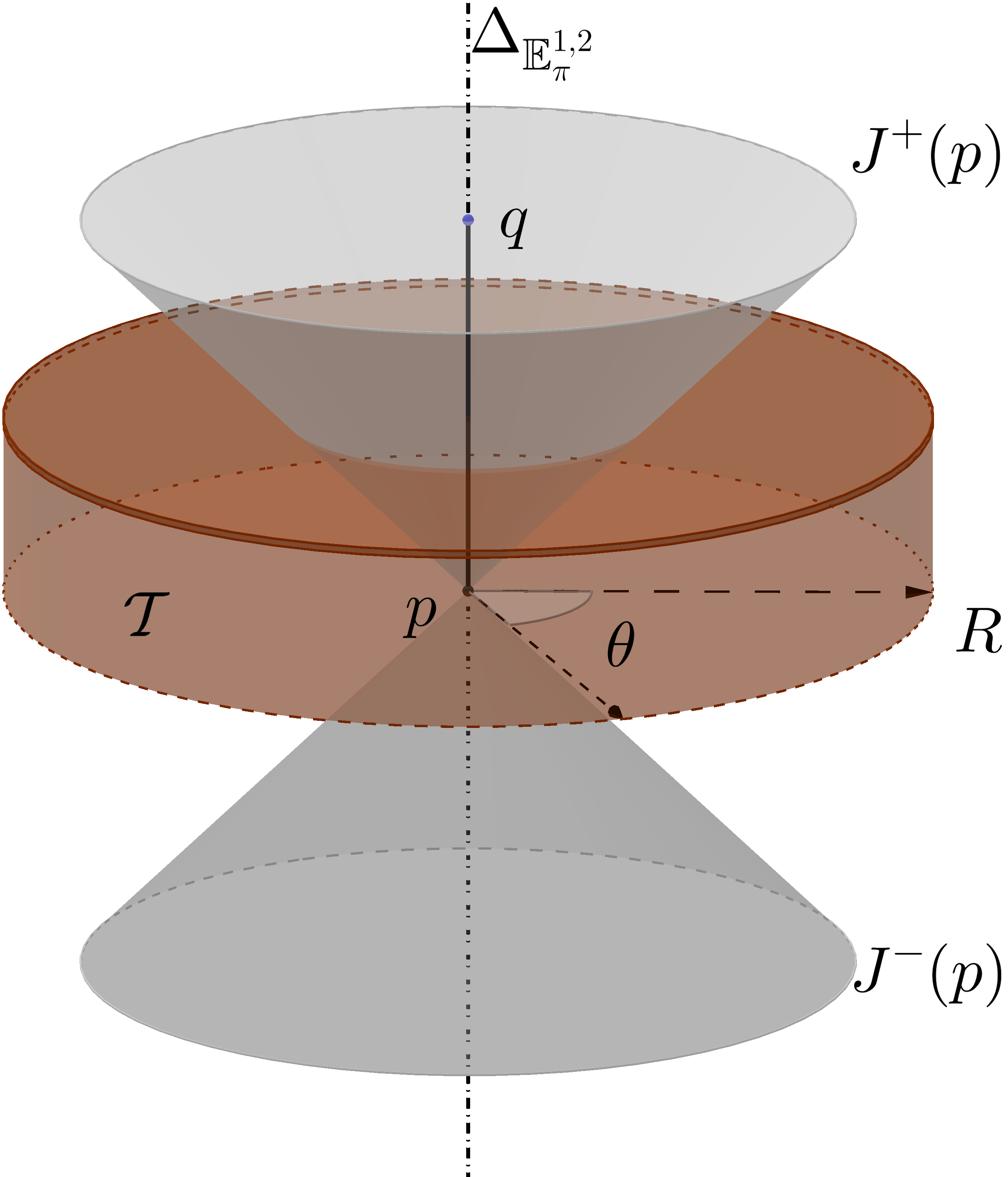
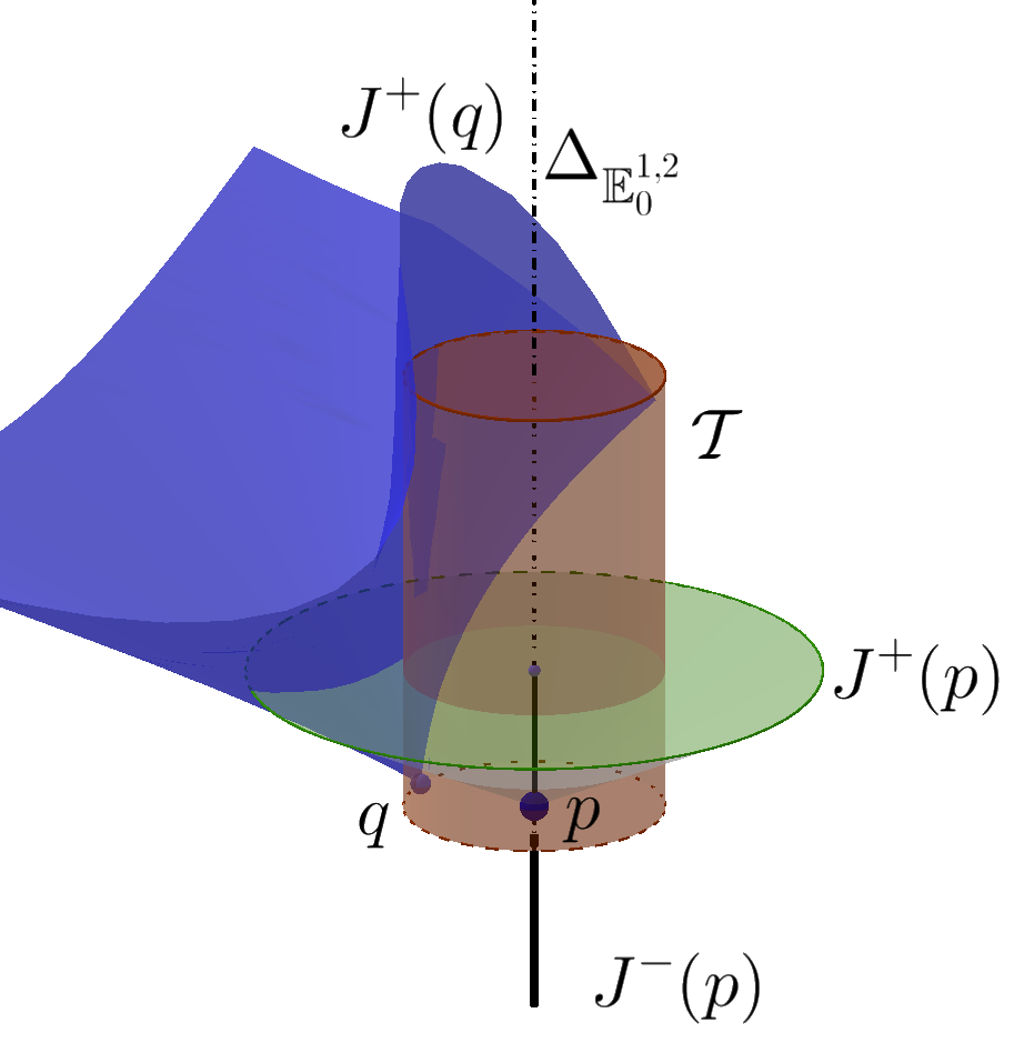
Figure 2: Causal cones in model spaces.

On the left is represented the model space $\mathbb{E}^{1,2}_{\pi}$. The vertical dotted line is the singular line $\Delta_{\mathbb{E}^{1,2}_{\pi}}$. On this line are represented two singular points $p$ and $q$ together with causal future and causal past of $p$ in grey. The segment $[p,q]$ is outlined. A tube $\mathcal{T}$ of radius $R$ is represented in brown The angular coordinate is represented by $\theta$. On the right is represented the model space $\mathbb{E}^{1,2}_{0}$ with the vertical dotted line as the singular line $\mathrm{Sing}(\mathbb{E}^{1,2}_{0})$. A singular point $p$ and a regular point $q$ are represented with their causal future. The causal future of $p$ is in green. We have depicted the tube $\mathcal{T}$ containing $q$ in his boundary. The blue surface is the union of future lightlike geodesics starting from $q$. It does not enter the tube $\mathcal{T}$. The causal past of $p$ is the black ray below $p$. The other part of the singular line is the dotted ray above $p$; it is the complement of $I^{+}(p)$ in the interior of $J^{+}(p)$.

1.4.2 Universal covering and developping map

Let $\alpha$ be a non-negative real number. If $\alpha>0$, the universal covering of $Reg(\mathbb{E}^{1,2}_{\alpha})$ can be naturally identified with

$$(\mathbb{R}\times\mathbb{R}^{*}_{+}\times\mathbb{R},-\mathrm{d}t^{2}+\mathrm{d}r^{2}+r^{2}\mathrm{d}\theta^{2}).$$

Definition 1.14.

Define

$$\mathbb{E}^{1,2}_{\infty}:=\left(\mathbb{R}\times\mathbb{R}_{+}^{*}\times\mathbb{R},-\mathrm{d}t^{2}+\mathrm{d}r^{2}+r^{2}\mathrm{d}\theta^{2}\right).$$

Let $\Delta$ be the vertical timelike line through the origin in $\mathbb{E}^{1,2}$, the group of isometries of $\mathbb{E}^{1,2}$ which sends $\Delta$ to itself is isomorphic to $\mathrm{SO}(2)\times\mathbb{R}$. The $\mathrm{SO}(2)$ factor corresponds to the set of linear isometries of axis $\Delta$ and $\mathbb{R}$ to the translations along $\Delta$. The group of isometries of $\mathbb{E}^{1,2}_{\infty}$ is then the universal covering of $\mathrm{SO}(2)\times\mathbb{R}$, namely $\mathrm{Isom}(\mathbb{E}^{1,2}_{\infty})\simeq\widetilde{\mathrm{SO}}(2)\times\mathbb{R}$. The regular part $Reg(\mathbb{E}^{1,2}_{\alpha})$ is then the quotient of $\mathbb{E}^{1,2}_{\infty}$ by the group of isometries generated by $(\tau,r,\theta)\mapsto(\tau,r,\theta+\alpha)$. We will simply write $\alpha\mathbb{Z}$ for this group. There is a natural choice of developping map $\mathcal{D}$ for $\mathbb{E}^{1,2}_{\infty}$ : the projection onto $\mathbb{E}^{1,2}_{\infty}/2\pi\mathbb{Z}$. Indeed, $\mathbb{E}^{1,2}_{\infty}/2\pi\mathbb{Z}$ can be identified with the complement of $\Delta$ in $\mathbb{E}^{1,2}$. In addition, $\mathcal{D}$ is $\rho$-equivariant with respect to the actions of $\mathrm{Isom}(\mathbb{E}^{1,2}_{\infty})$ and $\mathrm{Isom}(\mathbb{E}^{1,2})$ where $\rho$ is the projection onto $\mathrm{Isom}(\mathbb{E}^{1,2}_{\infty})/2\pi\mathbb{Z}\subset\mathrm{Isom}(\mathbb{E}^{1,2})$. The image of $\rho$ is then the group of rotation-translation around the line $\Delta$ with translation parallel to $\Delta$. This couple $(\mathcal{D},\rho)$ induces a developping map and an holonomy choice for the regular part of $\mathbb{E}^{1,2}_{\alpha}$ which is $(\mathcal{D},\rho_{|\alpha\mathbb{Z}})$. We get common constructions, developping map and holonomy for every $Reg(\mathbb{E}^{1,2}_{\alpha})$ simultaneously. Assume now $\alpha=0$ and let $\Delta$ be a lightlike line through the origin in $\mathbb{E}^{1,2}$. Notice that there exists a unique plane of perpendicular to $\Delta$ containing $\Delta$ since the direction of $\Delta$ is lightlike. Let $\Delta^{\perp}$ be the unique plane containing $\Delta$ and perpendicular to $\Delta$, we have $I^{+}(\Delta)=I^{+}(\Delta^{\perp})$. The causal future of $\Delta$ is $J^{+}(\Delta)=I^{+}(\Delta)\cup\Delta$. The isometries of $\mathbb{E}^{1,2}$ fixing $\Delta$ pointwise are parabolic isometries with a translation part in the direction of $\Delta$. The universal covering $\widetilde{Reg}(\mathbb{E}^{1,2}_{0})$ can be identified with $\mathbb{R}\times\mathbb{R}^{*}_{+}\times\mathbb{R}$ endowed with the metric $-2\mathrm{d}\tau\mathrm{d}r+\mathrm{d}r^{2}+r^{2}\mathrm{d}\theta^{2}$.

Proposition 1.15.

Let $\widetilde{Reg}({\mathbb{E}_{0}^{1,2}})$ be the universal covering of the regular part of ${\mathbb{E}_{0}^{1,2}}$.

• The developping map $\mathcal{D}:\widetilde{Reg}({\mathbb{E}_{0}^{1,2}})\rightarrow\mathbb{E}^{1,2}$ is injective;

• the holonomy sends the translation $(t,r,\theta)\mapsto(t,r,\theta+2\pi)$ to some parabolic isometry $\gamma$ which pointwise fixes a lightlike line $\Delta$;

• the image of $\mathcal{D}$ is the chronological future of $\Delta$.

Proof.

Parametrize $\widetilde{Reg}({\mathbb{E}_{0}^{1,2}})$ by $\left(\mathbb{R}\times\mathbb{R}_{+}^{*}\times\mathbb{R},-2\mathrm{d}\tau\mathrm{d}r+\mathrm{d}r^{2}+r^{2}\mathrm{d}\theta^{2}\right)$. The fundamental group of $Reg({\mathbb{E}_{0}^{1,2}})$ is generated by the translation $g:(\tau,r,\theta)\mapsto(\tau,r,\theta+2\pi)$. We use the carthesian coordinates of $\mathbb{E}^{1,2}$ in which the metric is $-\mathrm{d}t^{2}+\mathrm{d}x^{2}+\mathrm{d}y^{2}$. Let $\Delta=\mathbb{R}\cdot(1,1,0)$, let $\gamma$ be the linear parabolic isometry fixing $\Delta$ and sending $(0,0,1)$ on $(1,1,1)$. Then define

$$\mathcal{D}:\begin{array}[]{l|rcl}&\displaystyle\widetilde{Reg}({\mathbb{E}_{0}^{1,2}})&\longrightarrow&\displaystyle\mathbb{E}^{1,2}\\ &\displaystyle\left(\tau,r,\frac{\theta}{2\pi}\right)&\longmapsto&\displaystyle\begin{pmatrix}t\\ x\\ y\end{pmatrix}=\begin{pmatrix}\tau+\frac{1}{2}r\theta^{2}\\ \tau+\frac{1}{2}r\theta^{2}-r\\ -r\theta\end{pmatrix}\end{array}.$$

A direct computation shows that $\mathcal{D}$ is injective of image $I^{+}(\Delta)$ and one can see that

1. $\mathcal{D}$ is a $\mathbb{E}^{1,2}$-morphism ;

2. $\mathcal{D}(g\cdot(\tau,r,\theta))=\gamma\mathcal{D}(\tau,r,\theta)$.

From $(i)$, $\mathcal{D}$ is a developping map and from $(ii)$ the associated holonomy representation sends the translation $g$ to $\gamma$. ∎

Corollary 1.16.

We obtain a homeomorphism $\overline{\mathcal{D}}:Reg(\mathbb{E}^{1,2}_{0})\rightarrow I^{+}(\Delta)/\langle\gamma\rangle$

Remark 1.17.

Let $\mathcal{D}$ be a developping map of $Reg({\mathbb{E}_{0}^{1,2}})$, let $\gamma$ be a generator of the image of the holonomy associated to $\mathcal{D}$. Let $\lambda\in\mathbb{R}^{*}_{+}$ and let $h$ be a linear hyperbolic isometry of $\mathbb{E}^{1,2}$ which eigenspace associated to $\lambda$ is the line of fixed points of $\gamma$. The hyperbolic isometry $h$ defines an isometry $Reg({\mathbb{E}_{0}^{1,2}})\rightarrow Reg({\mathbb{E}_{0}^{1,2}})$. The pullback metric by $h$ is

$$\mathrm{d}s^{2}_{\lambda}=-2\mathrm{d}\tau\mathrm{d}r+\mathrm{d}r^{2}+\lambda^{2}r^{2}\mathrm{d}\theta^{2}.$$

Therefore, the above metric on $\mathbb{R}^{3}$ is isometric to ${\mathbb{E}_{0}^{1,2}}$ for every $\lambda>0$.

Remark 1.18.

This allows to generalizes remark 1.11 above. For all $\lambda>0$, the coordinates of ${\mathbb{E}_{0}^{1,2}}$ above induce a foliation $\{\tau=\tau_{0}\}$ for $\tau_{0}\in\mathbb{R}$. Each leaf is isometric to $\mathbb{E}^{2}_{\lambda}$.

Figure 3: Tubular neighborhood of a BTZ point and its development

On the left, a tubular subset of $\mathbb{E}^{1,2}_{0}$. On the right its development into $\mathbb{E}^{1,2}$. Colors are associated to remarkable sub-surfaces and their developments.

1.4.3 Rigidity of morphisms between model spaces

The next proposition is a rigidity property. A relatively compact subset of $\mathbb{E}^{1,2}$ embeds in every $\mathbb{E}^{1,2}_{\alpha}$, however we prove below that the regular part of a neighborhood of a singular point in $\mathbb{E}^{1,2}_{\alpha}$ ($\alpha\neq 2\pi$) cannot be embedded in any other $\mathbb{E}^{1,2}_{\beta}$. Furthermore, the embedding has to be the restriction of a global isometry of $\mathbb{E}^{1,2}_{\alpha}$. This proposition is central to the definition of singular spacetime.

Proposition 1.19.

Let $\alpha,\beta\in\mathbb{R}_{+}$ with $\alpha\neq 2\pi$, and let $\mathcal{U}$ be an open connected subset of $\mathbb{E}^{1,2}_{\alpha}$ containing a singular point and let $\phi$ be a continuous function $\mathcal{U}\rightarrow\mathbb{E}^{1,2}_{\beta}$. If the restriction of $\phi$ to the regular part is an injective $\mathbb{E}^{1,2}$-morphism then $\alpha=\beta$ and $\phi$ is the restriction of an element of $\mathrm{Isom}(\mathbb{E}^{1,2}_{\alpha})$.

Proof.

One can assume that $\mathcal{U}$ is a compact slice of tube around the singular line without loss of generality. We use the notation introduced in section 1.4.2. Assume $\alpha\beta\neq 0$. Lift $\phi$ to $\widetilde{\phi}:\widetilde{Reg}(\mathcal{U})\subset\mathbb{E}^{1,2}_{\infty}\rightarrow\mathbb{E}^{1,2}_{\infty}$ equivariant with respect to some morphism $\chi:\alpha\mathbb{Z}\rightarrow\beta\mathbb{Z}$. Writing $D$ the natural projection $\mathbb{E}^{1,2}_{\infty}\rightarrow\mathbb{E}^{1,2}$, $D_{|\widetilde{Reg}(\mathcal{U})}$ and $D\circ\widetilde{\phi}$ are two developping map of $Reg(\mathcal{U})$ and a thus equal up to composition by some isometry $\gamma\in\mathrm{Isom}(\mathbb{E}^{1,2})$, we will call the former standard and the latter twisted. Their image is a tube of respective axis $\Delta=\{r=0\}$ for the former and $\gamma\Delta$ for the latter. Furthermore, writing $\rho$ the projection of $\mathrm{Isom}(\mathbb{E}^{1,2}_{\infty})\rightarrow\mathrm{Isom}(\mathbb{E}^{1,2})$, $\gamma\cdot\rho_{|\alpha\mathbb{Z}}\cdot\gamma^{-1}=(\rho\circ\chi)$. Assume $\gamma\Delta\neq\Delta$, since the image of $D$ avoids $\Delta$, so does the twisted development of $\mathcal{U}$. It is then a slice of tube which does not intersect $\Delta$ and it is included in some half-space $H$ of $\mathbb{E}^{1,2}$ which support plane contains $\Delta$ the vertical axis. Then, by connectedness of $\mathcal{U}$, the image of $\widetilde{\phi}$ is included in some sector $\{\theta_{0}\leq\theta\leq\theta_{0}+\pi\}$. However, the image should be invariant under under $\chi(\alpha\mathbb{Z})$, and the only subgroup of $\beta\mathbb{Z}$ letting such a sector invariant is the trivial one. Consequently $\chi=0$, thus the lift $\phi:\mathcal{U}\rightarrow\mathbb{E}^{1,2}_{\infty}$ is well defined and $D\circ\widetilde{\phi}$ is injective, then so is $D_{|\widetilde{Reg}(\mathcal{U})}$. Furthermore, $\rho(\alpha)=0$, thus $\alpha=2\pi n$ for some $n$ greater than two. Then $D$ cannot be injective on some loop $\{r=\varepsilon,t=t_{0}\}$ in $\mathcal{U}$. Absurd. Thus $\gamma\Delta=\Delta$, the linear part of $\gamma$ is an elliptic element of axis $\Delta$ and the translation part of $\gamma$ is in $\Delta$. The isometry $\gamma$ is then in the image of $\rho$, one can then assume $\gamma=1$ by considering $\widetilde{\gamma}^{-1}\widetilde{\phi}$ intead of $\widetilde{\phi}$ with $\rho(\widetilde{\gamma})=\gamma$. In this case, $D\circ\widetilde{\phi}:=D$ then $\widetilde{\phi}$ is a translation of angle $2\pi n$, one can then choose the lift $\widetilde{\gamma}$ of $\gamma$ such that $n=0$. Consequently, $\widetilde{\phi}$ is the restriction to $\widetilde{Reg}(\mathcal{U})$ of an element of $\mathrm{Isom}(\mathbb{E}^{1,2}_{\infty})$, $\phi$ is then a covering and the morphism $\chi$ is then the restriction of the multiplication $\mathrm{Isom}(\mathbb{E}^{1,2}_{\infty})\xrightarrow{\times n}\mathrm{Isom}(\mathbb{E}^{1,2}_{\infty})$, then $\alpha\mathbb{Z}=n\beta\mathbb{Z}$ and using again the injectivity of $\phi$ on a standard loop, one get $\alpha=\beta$. Assume $\alpha\beta=0$, one obtain in the same way a morphism $\varphi$ such that $\rho_{\alpha}=\rho_{\beta}\circ\varphi$ induced by a lift $\widetilde{\phi}:\widetilde{\mathcal{U}}\subset\widetilde{Reg(\mathbb{E}^{1,2}_{\alpha})}\rightarrow\widetilde{Reg(\mathbb{E}^{1,2}_{\beta})}$. However, $\mathrm{Im}\rho_{\alpha}$ is generated by an elliptic isometry if $\alpha>0$ and a parabolic one if $\alpha=0$, then $\alpha$ cannot be zero if $\beta$ is not and reciprocally. Then $\alpha=\beta=0$. One again gets two developments of $\mathcal{U}$ the standard one and the one twisted by some $\gamma$, the standard image contains a horocycle around a lightlike line $\Delta$ and is invariant exactly under the stabilizer of $\Delta$. The twisted image is then invariant exactly under the stabilizer of $\gamma\Delta$. Therefore, the image of $\chi$ is in the intersection of the two and is non trivial. Remark that the only isometries $\gamma$ such that $\gamma\mathrm{Stab}(\Delta)\gamma^{-1}\cap\mathrm{Stab}(\Delta)\neq\{1\}$ are exactly $\mathrm{Stab}(\Delta)$. Finally, $\gamma$ stabilizes $\Delta$ and one can conclude the same way as before. ∎

Remark 1.20.

The core argument of the proof above shows that without the hypothesis of injectivity, $\phi$ shall be induced by a branched covering $\mathbb{E}^{1,2}_{\alpha}\rightarrow\mathbb{E}^{1,2}_{\beta}$. Thus $\alpha=n\beta$ for some $n$ and actually knowing that $\alpha=\beta$ gives that $\phi$ is an isomorphism if $\alpha\neq 0$. Beware that $\mathbb{E}^{1,2}_{0}$ is a branched covering of itself since, using cylindrical coordinates $\mathbb{R}\times\mathbb{R}_{+}\times\mathbb{R}/2\pi\mathbb{Z}$, the projection $\mathbb{R}/2\pi\mathbb{Z}\rightarrow\mathbb{R}/(\frac{2\pi}{p}\mathbb{Z})$, for instance, induces an isometric branched covering $\mathbb{R}\times\mathbb{R}_{+}\times\mathbb{R}/2\pi\mathbb{Z}\rightarrow\mathbb{R}\times\mathbb{R}_{+}\times\mathbb{R}/2\pi\mathbb{Z}$, the former with the metric $-\mathrm{d}\tau\mathrm{d}r+\mathrm{d}r^{2}+r^{2}\mathrm{d}\theta^{2}$ and the latter with the metric $-\mathrm{d}\tau\mathrm{d}r+\mathrm{d}r^{2}+\frac{1}{p^{2}}r^{2}\mathrm{d}\theta^{2}$. Both are coordinate systems of $\mathbb{E}^{1,2}_{0}$ from Remark 1.17. Thus one couldn’t get rid of the injectivity condition that easily.

1.5 Singular spacetimes

A singular spacetime is a patchwork of different structures. They can be associated with one another using their regular locus which is a natural $\mathbb{E}^{1,2}$-manifold. Such a patchwork must be given by an atlas identifying part of $M$ to an open subset of one of the model spaces, the chart must send regular part on regular part whenever they intersect and the regular locus must be endowed with a $\mathbb{E}^{1,2}$-structure.

Definition 1.21.

Let $A$ be a subset of $\mathbb{R}_{+}$. A $\mathbb{E}^{1,2}_{A}$-manifold is a second countable Hausdorff topological space $M$ with an atlas $\mathcal{A}=(\mathcal{U}_{i},\phi_{i})_{i\in I}$ such that

• For every $(\mathcal{U},\phi)\in\mathcal{A}$, there exists an open set $\mathcal{V}$ of $\mathbb{E}^{1,2}_{\alpha}$ for some $\alpha\in A$ such that $\phi:\mathcal{U}\rightarrow\mathcal{V}$ is a homeomorphism.

• For all $(\mathcal{U}_{1},\phi_{1}),(\mathcal{U}_{2},\phi_{2})\in\mathcal{A},$

  $$\phi_{2}\circ\phi^{-1}_{1}\left[Reg(\phi_{1}(\mathcal{U}_{2}\cap\mathcal{U}_{1}))\right]\subset Reg(\phi_{2}(\mathcal{U}_{1}\cap\mathcal{U}_{2}))$$

  and the restriction of $\phi_{2}\circ\phi^{-1}_{1}$ to $Reg(\phi_{1}(\mathcal{U}_{1}\cap\mathcal{U}_{2}))$ is a $\mathbb{E}^{1,2}$-morphism.

For $\alpha\in A\setminus\{2\pi\}$, $\mathrm{Sing}_{\alpha}$ denote the subset of $M$ that a chart sends to a singular point of $\mathbb{E}^{1,2}_{\alpha}$, and $\mathrm{Sing}_{2\pi}=\emptyset$.

In the following $A$ is a subset of $\mathbb{R}_{+}$ and $M$ is a $\mathbb{E}^{1,2}_{A}$-manifold. It is not obvious from the definition that a singular point in $M$ does not admit charts of different types. We need to prove the regular part $Reg(M)$ and the singular parts $\mathrm{Sing}_{\alpha}(M),\alpha\in\mathbb{R}_{+}$ form a well defined partition of $M$.

Proposition 1.22.

$\left(\mathrm{Sing}_{\alpha}\right)_{\alpha\in A}$ is a family of disjoint closed submanifolds of dimension 1.

Proof.

Let $\alpha\in\mathbb{R}_{+}\setminus\{2\pi\}$ and let $p\in\mathrm{Sing}_{\alpha}$ be a singular point, there exists a chart $\phi:\mathcal{U}\rightarrow\mathcal{V}$ around $p$ such that $\mathcal{V}\subset\mathbb{E}_{\alpha}$ and such that $\phi(p)\in\mathrm{Sing}(\mathbb{E}_{\alpha})$. For any other chart $\phi^{\prime}:\mathcal{U}^{\prime}\rightarrow\mathcal{V}^{\prime}$, $\phi^{\prime}\circ\phi^{-1}(Reg(\mathcal{V})\cap\phi(\mathcal{U}^{\prime}))\subset Reg(\mathcal{V}^{\prime})$ thus $\mathrm{Sing}_{\alpha}\cap\mathcal{U}=\phi^{-1}(\mathrm{Sing}(\mathbb{E}^{1,2}_{\alpha}))$. Since $\phi$ is a diffeomorphism and $\mathrm{Sing}(\mathbb{E}_{\alpha}^{1,2})$ is a closed 1-dimensional submanifold of $\mathbb{E}_{\alpha}^{1,2}$, so is $\mathrm{Sing}_{\alpha}\cap\mathcal{U}$. For $p\in Reg(M)$ and $\mathcal{U}$ a chart neighborhood of $p$, we have $\mathrm{Sing}_{\alpha}\cap\mathcal{U}=\emptyset$. Then $\mathrm{Sing}_{\alpha}$ is a closed 1-dimensional submanifold. Let $\alpha,\beta\in\mathbb{R}_{+}^{2}$ and assume there exists $p\in\mathrm{Sing}_{\alpha}\cap\mathrm{Sing}_{\beta}$. There exists charts $\phi_{\alpha}:\mathcal{U}_{\alpha}\rightarrow\mathcal{V}_{\alpha}$ $\phi_{\beta}:\mathcal{U}_{\beta}\rightarrow\mathcal{V}_{\beta}$ such that $\phi_{\alpha}(p)\in\Delta_{\mathbb{E}_{\alpha}^{1,2}}$ and $\phi_{\beta}(p)\in\Delta_{\mathbb{E}_{\beta}^{1,2}}$. Then, writing $\mathcal{V}_{\alpha}^{\prime}=Reg(\mathcal{V}_{\alpha}\cap\phi_{\alpha}(\mathcal{U}_{\beta}))$ and $\mathcal{V}_{\beta}^{\prime}=Reg(\mathcal{V}_{\beta}\cap\phi_{\beta}(\mathcal{U}_{\alpha}))$, $\phi_{\beta}\circ\phi_{\alpha}^{-1}:\mathcal{V}_{\alpha}^{\prime}\rightarrow\mathcal{V}^{\prime}_{\beta}$ is an isomorphism of $\mathbb{E}^{1,2}$-structures. Since $\mathcal{V}^{\prime}_{\alpha}$ is the regular part of an open subset of $\mathbb{E}^{1,2}_{\alpha}$ containing a singular point, from Proposition 1.19 we deduce that $\alpha=\beta$. ∎

Definition 1.23 (Morphisms and isomorphisms).

Let $M,N$ be $\mathbb{E}^{1,2}_{A}$-manifolds. A continous map $\phi:M\rightarrow N$ is a $\mathbb{E}_{A}^{1,2}$-morphism if $\phi_{|Reg(M)}^{|Reg(N)}:Reg(M)\rightarrow Reg(N)$ is a $\mathbb{E}^{1,2}$-morphism. A morphism $\phi$ is an isomorphism if it is bijective.

Consider a $\mathbb{E}^{1,2}_{A}$-structure $\mathcal{A}$ on a manifold $M$ and consider thiner atlas $\mathcal{A}^{\prime}$. The second atlas defines a second $\mathbb{E}^{1,2}_{A}$-structure on $M$. The identity is an isomophism between the two $\mathbb{E}^{1,2}_{A}$-structures, they are thus identified.

Proposition 1.24.

Let $M$ and $N$ be connected $\mathbb{E}_{A}^{1,2}$-manifolds. Let $\phi_{1},\phi_{2}:M\rightarrow N$ be two $\mathbb{E}^{1,2}_{A}$-morphisms. If there exists an open subset $\mathcal{U}\subset M$ such that $\phi_{1|\mathcal{U}}=\phi_{2|\mathcal{U}}$ then $\phi_{1}=\phi_{2}$.

Proof.

Since $M$ and $N$ are 3-dimensionnal manifolds and since $Sing(M)$ and $Sing(N)$ are embedded 1-dimensional manifolds, $Reg(M)$ and $Reg(N)$ are open connected and dense. Since $Reg(M)$ is a connected $\mathbb{E}^{1,2}$-structure, $\phi_{1|Reg(M)}=\phi_{2|Reg(M)}$. By density of $Reg(M)$ and continuity of $\phi_{1}$ and $\phi_{2}$, $\phi_{1}=\phi_{2}$. ∎

We end this section by an extension to singular manifold of a property we gave for the BTZ model space.

Lemma 1.25.

Let $M$ a $\mathbb{E}^{1,2}_{A}$-manifold then

• a connected component of $\mathrm{Sing}_{0}(M)$ is an inextendible causal curve ;

• every causal curve $c$ of $M$ decomposes into $c=\Delta\cup c^{0}$ where $\Delta=c\cap\mathrm{Sing}_{0}(M)$ and $c^{0}=c\setminus\mathrm{Sing}_{0}(M)$. Furthermore, $\Delta$ and $c^{0}$ are connected and $\Delta$ is in the past of $c^{0}$.

Proof.

A connected component $\Delta$ of $\mathrm{Sing}_{0}(M)$ is a 1-dimensional submanifold, connected and locally causal. Therefore, it is a causal curve. Since it is closed, it is also inextendible. Assume $\Delta$ is non empty and take some $p\in\Delta$. Let $q\in J^{-}(p)$ and let $c^{\prime}:[0,1]\rightarrow J^{-}(p)$ be a past causal curve such that $c^{\prime}(0)=p$ and $c^{\prime}(1)=q$. Then write :

$$I=\{s\in[0,1]\leavevmode\nobreak\ |\leavevmode\nobreak\ c([0,s])\subset\Delta\}.$$

• $0\in I$ so $I$ is not empty.

• Take $s\in I$, $c^{\prime}(s)$ is of type $\mathbb{E}^{1,2}_{0}$ and in a local chart $\mathcal{U}$, $J^{-}_{\mathcal{U}}(c^{\prime}(s))$ is in the singular line around $c^{\prime}(s)$. Thus for some $\varepsilon>0$, $c^{\prime}(]s,s+\varepsilon[)\subset\Delta_{c^{\prime}(s)}=\Delta$. Thus $[0,s+\varepsilon]\subset I$ and $I$ is open.

• Let $s=\sup I$, $c^{\prime}(]s-\varepsilon,s[)\subset S^{0}$. By closure of $S^{0}$, $\Delta$ is closed thus $c^{\prime}(s)\in\Delta$ and $s\in I$. Then $I$ is closed.

Finally, $I=[0,1]$ and $q\in\Delta$. We conclude that $\Delta$ is connected that there is no point of $c^{0}$ in the past of $\Delta$. ∎

2 Global hyperbolicity and Cauchy-extensions of singular spacetimes

We remind a Geroch characterisation of globally hyperbolic of regular spacetime and extend it to singular one. We extend the smoothing theorem of Bernal and Sanchez and the the Cauchy-Maximal extension theorem by Geroch and Choquet-Bruhat. We also prove that a BTZ line is complete in the future if the space-time is Cauchy-maximal.

2.1 Global hyperbolicity, Geroch characterisation

Let $M$ be a $\mathbb{E}_{A}^{1,2}$-manifold, the causality on $M$ is inherited from the causality and causal orientation of each chart, we can then speak of causal curve, acausal domain, causal/chronological future/past, etc. The chronological past/future are still open (maybe empty) since this property is true in every model spaces. We define global hyperbolicity, give the a Geroch splitting theorem and some properties.

Definition 2.1.

Let $P\subset M$ be a subset of $M$.

• The future Cauchy development of $P$ is the set

  $$D^{+}(P)=\{x\in M|\forall c:[0,+\infty[\rightarrow M\text{\leavevmode\nobreak\ inextendible past causal curve},c(0)=x\Rightarrow c\cap P\neq\emptyset\}$$

• The past Cauchy development of $P$ is the set

  $$D^{-}(P)=\{x\in M|\forall c:[0,+\infty[\rightarrow M\text{\leavevmode\nobreak\ inextendible future causal curve},c(0)=x\Rightarrow c\cap P\neq\emptyset\}$$

• The Cauchy development of $P$ is the set $D(P)=D^{+}(P)\cup D^{-}(P)$

Definition 2.2 (Cauchy Surface).

A Cauchy-surface in a $\mathbb{E}^{1,2}_{A}$-manifold is a $\mathscr{C}^{0}$-surface $\Sigma\subset M$ such that all inextendible causal curves intersects $\Sigma$ exactly once.

In particular if $\Sigma$ is a Cauchy-surface of $M$ then $\mathcal{D}(\Sigma)=M$.

Definition 2.3 (Globally hyperbolic manifold).

If a $\mathbb{E}^{1,2}_{A}$-manifold has a Cauchy-surface, it is globally hyperbolic.

The following theorem gives a fundamental charaterisation of globally hyperbolic spacetimes. Neither Geroch nor Bernal and Sanchez have proved this for singular manifolds but the usual arguments apply. The method is to define a time function as a volume function :

$$T(x)=\ln\frac{\mu(I^{-}(x))}{\mu(I^{+}(x))}$$

where $\mu$ is a finite measure on a spacetime $M$. Usually, one uses an absolutely continuous measure, however such a measure put a zero weight on the past of a BTZ point. The solution in the presence of BTZ lines is to put weight on the BTZ lines and choosing a measure which is the sum of a 3 dimensional absolutely continuous measure on $M$ and a 1 dimensional absolutely continuous measure on $\mathrm{Sing}_{0}(M)$. The definition of causal spacetime along with an extensive exposition of the hierachy of causality properties can be found in [MS08] and a direct exposition of basic properties of such volume functions in [Die88].

Theorem 2.1 ([Ger70],[BS07]).

Let $M$ be a $\mathbb{E}^{1,2}_{A}$-manifold, $(i)\Leftrightarrow(ii)$.

1. $M$ is globally hyperbolic.

2. $M$ is causal and $\forall p,q\in M,\overline{\Diamond}_{p}^{q}$ is compact.

Proposition 2.4.

If $\Sigma$ is a Cauchy-surface of $M$ then there exists a homeomorphism $M\xrightarrow{\phi}\mathbb{R}\times\Sigma$ such that for every $C\in\mathbb{R}$, $\phi^{-1}(\{C\}\times\Sigma)$ is a Cauchy-surface.

Proof.

See [O’N83] ∎

The topology generated by the open diamonds $\Diamond_{p}^{q}$ is called the Alexandrov topology. In the case of globally hyperbolic spacetimes, the Alexandrov topology coincides with the standard topology on the underlying manifold.

Lemma 2.5.

Let $M$ be a globally hyperbolic $\mathbb{E}^{1,2}_{A}$-manifold and let $K_{1},K_{2}$ be compact subsets. Then

• $J^{+}(K_{1})\cap J^{-}(K_{2})$ is compact ;

• $J^{+}(K_{1})$ and $J^{-}(K_{2})$ are closed.

Proof.

The usual arguments apply since they can be formulated using only the Alexandrov topology, the compactness of closed diamonds and the metrisability of the topology. Let $(x_{n})_{n\in\mathbb{N}}$ be a sequence in $J^{+}(K_{1})\cap J^{-}(K_{2})$, there exists sequences $(p_{n})_{n\in\mathbb{N}}\in K_{1}^{\mathbb{N}}$ and $(q_{n})_{n\in\mathbb{N}}\in K_{2}^{\mathbb{N}}$ such that $x_{n}\in\overline{\Diamond}_{p_{n}}^{q_{n}}$ for all $n\in\mathbb{N}$. Extracting a subsequence if necessary, one can assume $p_{n}\xrightarrow{n\rightarrow+\infty}p$ and $q_{n}\xrightarrow{n\rightarrow+\infty}q$ for some $p\in K_{1}$ and $q\in K_{2}$. There exists a neighborhood of $p$ of the form $J^{+}(p^{\prime})$ and a neighborhood of $q$ of the form $J^{-}(q^{\prime})$ for some $p^{\prime}$ and $q^{\prime}$. The sequences $(p_{n})_{n\in\mathbb{N}}$ and $(q_{n})_{n\in\mathbb{N}}$ enters respectively $J^{+}(p^{\prime})$ and $J^{-}(q^{\prime})$, then for $n$ big enough, $x_{n}\in\overline{\Diamond}_{p^{\prime}}^{q^{\prime}}$. This subset is compact, thus one can extract a subsequence of $(x_{n})_{n\in\mathbb{N}}$ converging to some $x_{\infty}\in\overline{\Diamond}_{p^{\prime}}^{q^{\prime}}$. Take a sequence $(p^{\prime}_{n})_{n\in\mathbb{N}}$ of such $p^{\prime}$’s converging toward $p$ and a sequence $(q^{\prime}_{n})_{n\in\mathbb{N}}$ of such $q^{\prime}$’s converging toward $q$. Since each $J^{+}(p^{\prime}_{n})$ is a neighborhood of $p$ and each $J^{-}(q^{\prime}_{n})$ is a neighborhood of $q$ then forall $n$, $x_{k}\in\overline{\Diamond}_{p^{\prime}_{n}}^{q^{\prime}_{n}}$ for $k$ big enough. Finally, by compactness of $\overline{\Diamond}_{p^{\prime}_{n}}^{q^{\prime}_{n}}$, the limit

$$x_{\infty}\in\bigcap_{n\in\mathbb{N}}\overline{\Diamond}_{p^{\prime}_{n}}^{q^{\prime}_{n}}=\overline{\Diamond}_{p}^{q}\subset J^{+}(K_{1})\cap J^{-}(K_{2})$$

Let $x_{n}\xrightarrow{n\rightarrow+\infty}x$ be a converging sequence of points of $J^{+}(K_{1})$. There exists a neighborhood of $x$ of the form $J^{-}(q)$, by global hyperbolicity of $M$, $J^{-}(q)\cap J^{+}(K_{1})$ is compact and contains every points of $x_{n}$ for $n$ big enough. Thus $x\in J^{-}(q)\cap J^{+}(K_{1})$ and $x\in J^{+}(K_{1})$. We prove the same way that $J^{-}(K_{2})$ is closed. ∎

2.2 Cauchy-extension and Cauchy-maximal singular spacetimes

Extensions and maximality of spacetimes are usually defined via Cauchy-embeddings as follows.

Definition 2.6 (Cauchy-embeddings).

Let $M_{1},M_{2}$ be globally hyperbolic $\mathbb{E}^{1,2}_{A}$-manifolds and let $\phi:M_{1}\rightarrow M_{2}$ be a morphism. $\phi$ is a Cauchy-embedding if it is injective and sends a Cauchy-surface of $M_{1}$ on a Cauchy-surface of $M_{2}$.

The definition can be loosen twice, first by only imposing the existence of a Cauchy-surface of $M_{1}$ that $\phi$ sends to a Cauchy-surface of $M_{2}$, it is an exercise to prove that this implies that every Cauchy-surfaces is sent to a Cauchy-surface. Second, injectivity along a Cauchy-surface implies injectivity of $\phi$. We remind that a spacetime is Cauchy-maximal if every Cauchy-extension is trivial. The proof of the Cauchy-maximal extension theorem given by Choquet-Bruhat and Geroch have been improved by Jan Sbierski in [Sbi15]. This new proof has the advantage of not using Zorn’s lemma, it is thus more constructive. The existence and uniqueness of a Maximal Cauchy-extension of a singular spacetime can be proven re-writing the proof given by Sbierski taking some care with the particles. Indeed, it is shown in [BBS11] that collisions of particles can make the uniqueness fail. The rigidity Proposition 1.19 ensures the type of particles is preserved and is an equivalent of local uniqueness of the solution of Einstein’s Equation in our context. The proof of separation given by Sbierski has to be adapted to massive particles of angle greater than $2\pi$ to fully work. It can be done without difficulties and the main ideas of the proof are used in section 3.1 for BTZ extensions, so we don’t rewrite a proof of the theorem here.

Theorem 2.2 (Cauchy-Maximal extension).

Let $M$ be a globally hyperbolic $\mathbb{E}^{1,2}_{A}$-manifold. Then, there exists a maximal Cauchy-extension of $M$ among $\mathbb{E}^{1,2}_{A}$-manifold. Furthermore, it is unique up to isomorphism.

Proof.

See [Sbi15]. ∎

We now prove in a Cauchy-maximal spacetime a BTZ line is complete in the future and there is a standard neighborhood of a future BTZ ray.

Proposition 2.7.

Let $M$ be Cauchy-maximal $\mathbb{E}^{1,2}_{A}$-manifold and let $p$ be a BTZ point in $\mathrm{Sing}_{0}(M)$. Then, the future BTZ ray from $p$ is complete and there exists a future half-tube neighborhood of $[p,+\infty[$ of constant radius.

Proof.

Consider $\Sigma$ a Cauchy-surface of $M$. The connected component $\Delta$ of $p$ in $\mathrm{Sing}_{0}(M)$ is an inextendible causal curve thus it intersects the Cauchy-surface $\Sigma$ exactly once say at $q\in\Sigma\cap\Delta$. There exists a neighborhood $\overline{\mathcal{U}}$ of $q$ isomorphic via some isometry $\phi:\overline{\mathcal{U}}\rightarrow\mathbb{E}^{1,2}_{0}$ to

$$\{\tau\in[\tau_{1},\tau_{2}],r\leq R\}\subset\mathbb{E}^{1,2}_{0}$$

for some positive $R$ and reals $\tau_{1},\tau_{2}\in\mathbb{R}$. Take this neighborhood small enough so that the surface $\{\tau=\tau_{2},r<R\}$ is achronal in $M$. Consider the open tube $\mathcal{T}=\{\tau>\tau_{1},r<R\}\subset\mathbb{E}^{1,2}_{0}$ and $\mathcal{U}=Int(\overline{\mathcal{U}})$. Define

• $M_{0}=M\setminus J^{+}\left(\phi^{-1}(\{\tau=\tau_{2},r\leq R\})\right)$ ;

• $M_{2}=\left(M_{0}\coprod\mathcal{T}\right)/\sim$ with $x\sim y\Leftrightarrow\left(x\in\mathcal{U},y\in\mathcal{T}\text{ and }\phi(x)=y\right)$.

$\Sigma$ is a Cauchy-surface of $M_{0}$ and $M$ is Cauchy-extension of $M_{0}$. In order to prove that $M_{2}$ is a $\mathbb{E}^{1,2}_{A}$-manifold, we only need to prove it is Hausdorff. Indeed $\phi$ is an isomorphism thus the union of the atlases of $M_{0}$ and $\mathcal{T}$ defines a $\mathbb{E}^{1,2}_{A}$-structure on $M_{2}$.
Claim : $M_{2}$ is Hausdorff.
Let $x,y\in M_{2}$, $x\neq y$ and let $\pi$ be the natural projection $\pi:M_{0}\coprod\mathcal{T}\rightarrow M_{2}$. If $x,y\in\pi(\mathcal{U})$, consider $x_{1}=\pi^{-1}(x)\cap\mathcal{U}$, $x_{2}=\pi^{-1}(x)\cap\mathcal{T}$, $y_{1}=\pi^{-1}(y)\cap\mathcal{U}$, $y_{2}=\pi^{-1}(y)\cap\mathcal{T}$. Consider disjoint open neighborhoods $\mathcal{V}_{x_{1}}$ and $\mathcal{V}_{y_{1}}$ of $x_{1}$ and $y_{1}$. Notice that $\mathcal{V}_{x}:=\pi^{-1}(\pi(\mathcal{V}_{x_{1}}))=\mathcal{V}_{x_{1}}\cup\phi(\mathcal{V}_{x_{1}})$ and that $\mathcal{V}_{y}:=\pi^{-1}(\pi(\mathcal{V}_{y_{1}}))=\mathcal{V}_{y_{1}}\cup\phi(\mathcal{V}_{y_{1}})$. Therefore $\mathcal{V}_{x}$ and $\mathcal{V}_{y}$ are open and disjoint neighborhoods of $x$ and $y$. Notice that $\pi^{-1}(\overline{\pi(\mathcal{U})})=\overline{\mathcal{U}}\cup\{\tau\in]\tau_{1},\tau_{2}],r<R\}$. Clearly, if $x$ and $y$ are in $M_{2}\setminus\overline{\pi(\mathcal{U})}$, then they are separated. Then remains when $x,y\in\partial\pi(\mathcal{U})=\pi(\partial\mathcal{U}))\cup\pi(\{\tau=\tau_{2}\})$. Assume $x,y\in\partial\pi(\mathcal{U})$ and consider $x_{1}\in\overline{\mathcal{U}}$, $y_{1}\in\overline{\mathcal{U}}$ such that $\pi(x_{1})=x$ and $\pi(y_{1})=y$. Take two disjoint open neighborhoods $\mathcal{V}_{x_{1}}$ and $\mathcal{V}_{y_{1}}$ of $x_{1}$ and $y_{1}$ in $M_{0}$. We have $\pi^{-1}(\pi(\mathcal{V}_{x_{1}}))=\mathcal{V}_{x_{1}}\cup\phi(\mathcal{V}_{x_{1}}\cap\mathcal{U})$ and $\pi^{-1}(\pi(\mathcal{V}_{y_{1}}))=\mathcal{V}_{y_{1}}\cup\phi(\mathcal{V}_{y_{1}}\cap\mathcal{U})$. Then $x$ and $y$ are separated. The same way, we can separate two points $x,y\in\pi(\{\tau=\tau_{2},r<R\})$. Assume $x=\pi(x_{1})$ with $x_{1}\in\partial\overline{\mathcal{U}}$ and $y=\pi(y_{1})$ with $y_{1}\in\{\tau=\tau_{2},r<R\}$. The point $x_{1}$ is not in $\phi^{-1}(\{\tau=\tau_{2}\})$ by definition of $M_{0}$. Therefore, the $\tau$ coordinate of $\phi(x_{1})$ is less than $\tau_{2}$. Take a neighborhood $\mathcal{V}_{x_{1}}$of $x_{1}$ such that $\phi(\mathcal{V}_{x_{1}}\cap\mathcal{U})\subset\{\tau<\tau_{2}-\varepsilon\}$ for some $\varepsilon>0$. Then, take $\mathcal{V}_{y_{2}}=\{\tau>\tau_{2}-\varepsilon,r<R\}$. We get $\pi^{-1}(\pi(\mathcal{V}_{x_{1}}))=\mathcal{V}_{x_{1}}\cup\phi(\mathcal{U}\cap\mathcal{V}_{x_{1}})$ and $\pi^{-1}(\pi(\mathcal{V}_{x_{2}}))=\mathcal{V}_{x_{2}}\cup\phi^{-1}(\{\tau\in]\tau_{2}-\varepsilon,\tau_{2}[\})$. Therefore, $\pi(\mathcal{V}_{x_{1}})$ and $\pi(\mathcal{V}_{y_{1}})$ are open and disjoint. Finally, $M_{2}$ is Hausdorff. Consider a future inextendible causal curve in $M_{2}$ say $c$ and write $\Pi=\{\tau=\tau_{2},r<R\}\subset\mathcal{T}$. The curve $c$ can be decomposed into two part : $c_{0}=c\cap M_{0}$ and $c_{1}=c\cap J^{+}(\pi(\{\tau=\tau_{2},r<R\}))$. These pieces are connected since $\Pi$ is achronal in $\mathcal{T}$ and $\phi^{-1}(\Pi)$ is achronal in $M$. Therefore, $c_{1}$ and $c_{0}$ are inextendible causal curves if not empty. if $c_{1}$ is non empty, then it intersects $\Pi$ since $D^{+}_{\mathcal{T}}(\Pi)=\{\tau\geq\tau_{2},r<R\}$ and then $c_{0}$ is non empty. Therefore, $c_{0}$ is always non empty. $c_{1}$ does not intersect $\Sigma$ and $c_{0}$ interests $\Sigma$ exactly once thus $c$ interests $\Sigma$ exactly once. We obtain the following diagram of extensions by maximality of $M$

where the arrows are Cauchy-embedding. Therefore, the connected component of $p$ in $\mathrm{Sing}_{0}(M)$ is complete in the future and has a neighborhood isomorphic to $\mathcal{T}$. ∎

2.3 Smoothing Cauchy-surfaces in singular space-times

The question of the existence of a smooth Cauchy-surface of a regular globally hyperbolic manifold has been the object of many endeavours. Seifert [Sei33] was the first one to ask wether the existence of a $\mathscr{C}^{0}$ Cauchy-surface was equivalent to the existence of a $\mathscr{C}^{1}$ one, he gave an proof which turns out to be wrong. Two recent proofs are considered (so far) to be correct : one of Bernal and Sanchez [BS03] and another by Fathi and Siconolfi [FS12] . We give their result in the case of $\mathbb{E}^{1,2}$-manifolds.

Theorem 2.3 ([BS03] ).

Let $M$ be a globally hyperbolic $\mathbb{E}^{1,2}$-manifold, then there exists a spacelike smooth Cauchy-surface of $M$.

We apply their theorem to a globally hyperbolic flat singular spacetime. First we need to define what we mean by spacelike piecewise smooth Cauchy-surfaces. Recall that a smooth surface in $\mathbb{E}^{1,2}$ is spacelike if the restriction of the Lorentzian metric to its tangent plane is positive definite.

Definition 2.8.

Let $M$ be a globally hyperbolic $\mathbb{E}^{1,2}_{A}$-manifold and let $\Sigma$ be a Cauchy-surface of $M$.

• $\Sigma$ is smooth (resp. piecewise smooth) if $\Sigma\cap Reg(M)$ is smooth (resp. piecewise smooth);

• $\Sigma$ is spacelike (piecewise) smooth $\Sigma\cap Reg(M)$ is (piecewise) smooth and spacelike.

Theorem I.

Let $M$ be a globally hyperbolic $\mathbb{E}^{1,2}_{A}$-manifold, then there exists a spacelike smooth Cauchy-surface of $M$.

Proof.

Let $\Sigma_{1}$ be a Cauchy surface of $M$.

• Let $\left(\Delta_{i}\right)_{i\in\Lambda}$ be the connected components of $\mathrm{Sing}_{0}(M)$. Each connected component is an inextendible causal curve intersecting $\Sigma_{1}$ exactly once. Let $p_{i}=\Delta_{i}\cap\Sigma_{1}$ for $i\in\Lambda_{0}$. Let $i\in\Lambda_{0}$, consider $\mathcal{U}_{i}\simeq\{\tau\in[\tau^{-}_{i},\tau^{+}_{i}],r\leq R_{i}\}$ a tube neighborhood of $p_{i}$. Let $\mathbb{D}_{i}^{-}=\{\tau=\tau^{-}_{i},r\leq R\}$. The past set $I^{-}(\Sigma_{1}\cap\mathcal{U}_{i})$ is an open neighborhood of the ray $J^{-}(p_{i})\setminus\{p_{i}\}$. Therefore, noting $q_{i}=\mathbb{D}^{-}_{i}\cap J^{-}(p_{i})$, the past of $\Sigma_{1}$ contains a neighborhood of $q_{i}$ in $\mathbb{D}_{i}$. Reducing $R_{i}$ if necessary, one can assume $\mathbb{D}_{i}^{-}\subset I^{-}(\Sigma_{1})$ and reducing $R_{i}$ even more we can assume $\mathbb{D}_{i}^{+}:=\{\tau=\tau_{i}^{+},r\leq R_{i}\}\subset J^{+}(p_{i})$. In the same way, we index the connected components of the set of massive particles by $\Lambda_{\text{mass}}$. We have $\bigcup_{\alpha>0}\mathrm{Sing}_{\alpha}(M)=\bigcup_{j\in\Lambda_{\text{mass}}}(\Delta_{j})$ and $p_{j}=\Delta_{j}\cap\Sigma_{1}$ for $j\in\Lambda_{\text{mass}}$. Since $\Lambda\cup\Lambda_{\text{mass}}$ is enumerable, one can construct $(U_{i_{n}})_{n\in\mathbb{N}}$ by induction such that for all $n\in\mathbb{N}$, $\mathcal{U}_{i_{n+1}}$ is disjoint from $J^{\pm}(\mathcal{U}_{i_{k}})$ for $k\leq n$. Then define

  $$N=\left(\bigcup_{i\in\Lambda}J^{+}(\mathbb{D}^{+}_{i})\cup J^{-}(\mathbb{D}_{i}^{-})\right)\cup\left(\bigcup_{j\in\Lambda_{\text{mass}}}J^{+}(p_{j})\cup J^{-}(p_{j})\right)$$

  and

  $$M^{\prime}=Reg(M\setminus N).$$

  The closed dimonds of $M^{\prime}$ are compact, thus by Theorem 2.1, $M^{\prime}$ is a globally hyperbolic $\mathbb{E}^{1,2}$-manifold. Theorem 2.3 then ensures there exists a smooth Cauchy surface $\Sigma_{2}$ of $M^{\prime}$. We need to extend $\Sigma_{2}$ to get a Cauchy-surface of $M$.

• We write $\mathbb{D}_{R}$ the compact disc of radius $R$ in $\mathbb{E}^{2}$ and $\mathbb{D}_{R}^{*}:=\mathbb{D}_{R}\setminus\{0\}$. Consider a massive particle point $p_{j}$ for some $j\in\Lambda_{\text{mass}}$ and a tube neighborhood $\mathcal{U}\simeq\{t\in[t^{-},t^{+}],r\leq R\}$ of $p_{j}$ in $M$. We may assume the $t$ coordinate of $p_{j}$ to be $0$, $t^{-}=-t^{+}$ and $R=t^{+}$ so that $\{t=t^{+}\}$ is exactly the basis of the cone $J^{+}(p_{j})$ in $\mathcal{U}$ and $\{t=t^{-}\}$ is exactly the basis of the cone $J^{-}(p_{j})$ in $\mathcal{U}$. Consider the projection

  $$\pi:\begin{array}[]{l|rcl}&\displaystyle(\Sigma_{2}\cap\mathcal{U})\cup\{p_{j}\}&\longrightarrow&\displaystyle\mathbb{D}_{R}\\ &\displaystyle(t,r,\theta)&\longmapsto&\displaystyle(r,\theta)\end{array}$$

  where $(t,r,\theta)$ are the cylindrical coordinates of $\mathcal{U}$. The projection $\pi$ is continuous. Notice that for $r_{0}\in]0,R]$ and $\theta_{0}\in\mathbb{R}/2\pi\mathbb{Z}$, the causal curves $\{r=r_{0},\theta=\theta_{0},t\in]-r_{0},r_{0}[\}$ are inextendible in $M^{\prime}$. They thus intersect $\Sigma_{2}$ exactly once and $\pi$ is thus bijective. Let $(q_{n})_{n\in\mathbb{N}}$ be a sequence of points of $\Sigma$ such that the $r$ coordinates tends to $0$. Writing $r_{n}$ and $t_{n}$ the $r$ and $t$ coordinates of $q_{n}$ for $n\in\mathbb{N}$, we have $|t_{n}|<r_{n}$ thus $q_{n}\rightarrow p_{j}$. Since $\mathcal{U}$ is compact, $\Sigma_{2}\cap\mathcal{U}\cap\{r\geq R_{1}\}$ is compact, it follows that $(\Sigma_{2}\cap\mathcal{U})\cup\{p_{j}\}$ is compact. Then $\pi$ is a homeomorphism.Consider now a BTZ point $p_{i}$ for some $i\in\Lambda_{0}$ and a chart neighborhood of $p_{i}$ as in the first step. Again, the Cauchy-surface $\Sigma_{2}$ is trapped between $\mathbb{D}^{+}_{i}$ and $\mathbb{D}_{i}^{-}$, the projection $\pi:\Sigma_{2}\cap\mathcal{U}\rightarrow\mathbb{D}_{R}^{*}$ is bijective and open thus a homeomorphism. Write $\pi^{-1}=(\tau,Id)$ and let $(a_{n})_{n\in\mathbb{N}},(b_{n})_{n\in\mathbb{N}}$ be two sequences of points of $\mathbb{D}_{R}^{*}$ which tend to $0$. By compactness, we can assume $\left(\tau(a_{n})\right)_{n\in\mathbb{N}}$ and $\left(\tau(b_{n})\right)_{n\in\mathbb{N}}$ converge to some $\tau_{a}$ and $\tau_{b}$ respectively. If $\tau_{a}<\tau_{b}$ then for $n$ big enough $(\tau_{a},0))\in I^{-}(\pi^{-1}(b_{n}))$ which is open. Therefore, there exists $n,m\in\mathbb{N}$ such that $\pi^{-1}(a_{n})\in I^{-}(\pi^{-1}(b_{m}))$. Since $\Sigma_{2}$ is acausal this is absurd and $\tau_{a}=\tau_{b}$. Then $\pi^{-1}$ can be extended to a homeomorphism $\mathbb{D}_{R}\rightarrow\left(\Sigma_{2}\cap\mathcal{U}\right)\cup\{q_{i}\}$ for some $q_{i}\in\Delta_{i}$. Define $\Sigma=\Sigma_{2}\cup\{p_{j}:j\in\Lambda_{\text{mass}}\}\cup\{q_{i}:i\in\Lambda\}=\overline{\Sigma}_{2}$, it is a topological surface smooth on the regular part.

• We need to show $\Sigma_{2}$ is a Cauchy-surface of $M$. Let $c$ be a future causal inextendible curve in $M$. Notice that $N$ can be decomposed

  $$N=N^{+}\cup N^{-}\quad\text{where}\quad N^{\pm}=\bigcup_{i\in\Lambda_{0}}J^{\pm}(\mathbb{D}_{i}^{\pm})\bigcup_{j\in\Lambda_{\text{mass}}}J^{\pm}(\{p_{j}\})$$

  is the future complete part (the union of the $J^{+}$ parts) and $N^{-}$ is the past complete part (the union of the $J^{-}$ parts). A future causal curve entering $N^{+}$ cannot leave $N^{+}$ and a future causal curve leaving $N^{-}$ cannot re-enter $N^{-}$. Therefore, $c$ is decomposed into three connected pieces $c=c^{-}\cup c^{0}\cup c^{+}$, the pieces $c^{-},c^{0},c^{+}$ being in $N^{-}$, $M\setminus N$ and $N^{+}$ respectively.

  • If $c^{0}=\emptyset$ then $c\subset nN$ thus $c\cap\Sigma_{1}\subset N\cap\Sigma=\bigcup_{j\in\Lambda_{\text{mass}}}\{p_{j}\}$. The curve $c$ can then only intersect $\Sigma$ at a massive particle point, but such points of $\Sigma$ are in $\Sigma_{1}$ which is a Cauchy-surface of $M$. Therefore, $c$ intersects $\Sigma$ exactly once at $p_{j}$ for some $j\in\Lambda_{\text{mass}}$.

  • If $c^{0}\neq\emptyset$, then by Lemma 1.13, $c^{0}$ decomposes into a BTZ part $\Delta$ and a non BTZ-part $c^{1}$ with $\Delta$ in the past of $c^{1}$. Then $c=c^{-}\cup\Delta\cup c^{1}\cup c^{+}$.

    • If $c^{1}\neq\emptyset$, then $c^{1}$ is an inextendible causal curve in $M^{\prime}$ and thus intersect $\Sigma_{2}$, thus $\Sigma$, exactly once. If $q_{i}\in\Delta$ for some $i\in\Lambda_{0}$, then $q_{i}\in J^{-}_{M}(\Sigma_{2})\setminus\Sigma_{2}=I^{-}(\Sigma_{2})$. However, $I^{-}(\Sigma_{2})$ is open and $q_{i}\in\overline{\Sigma_{2}}$, thus $I^{-}(\Sigma_{2})\cap\Sigma_{2}\neq\emptyset$ which is absurd since $\Sigma_{2}$ is acausal in $M^{\prime}$. Thus $c\cap\Sigma=c^{1}\cap\Sigma$ which is a singleton.

    • If $c^{1}=\emptyset$, then $\Delta$ is inextendible and thus a connected component of $\mathrm{Sing}_{0}(M\setminus N)$. Such a connected component contains exactly one of the $(q_{i})_{i\in\Lambda}$ thus $c\cap\Sigma=\Delta\cap\Sigma$ is a singleton.

∎

Lemma 2.9.

Let $\Sigma$ a picewise spacelike Cauchy-surface of $M$ and write $\mathbb{D}_{R}=\{r\leq R\}\subset\mathbb{E}^{2}$. For all $p\in\Sigma$, there exists a tube neighborhood $\mathcal{U}\simeq\mathcal{T}\subset\mathbb{E}^{1,2}_{\alpha}$ of $p$ such that

• $\mathcal{T}=\{\tau\in[\tau_{1},\tau_{2}],r\leq R\}$ if $\alpha=0$ ;

• $\mathcal{T}=\{t\in[t_{1},t_{2}],r\leq R\}$ if $\alpha>0$ ;

• $\Sigma\cap\mathcal{U}=\{(f(r,\theta),r,\theta):(r,\theta)\in\mathbb{D}_{R}\}$ for some $f:\mathbb{D}_{R}\rightarrow\mathbb{R}$ which is piecewise smooth on $\mathbb{D}_{R}^{*}$.

Proof.

Steps 1 and 2 of the proof of Theorem I give a continuous parametrisation. The parametrisation is piecewise smooth since the projection is along lightlike line or timelike line which are transverse to the spacelike Cauchy-surface. ∎

The Riemann metric on $Reg(\Sigma)$ induces a length space structure on $Reg(\Sigma)$ and a distance function on $Reg(\Sigma)\times Reg{\Sigma}$. In the next proposition, we extend this length space structure on the whole $\Sigma$ by proving $C^{1}_{pw}$ curve to the whole $\Sigma$

Proposition 2.10.

Let $M$ be a globally hyperbolic $\mathbb{E}^{1,2}_{A}$-manifold and let $\Sigma$ a piecewise smooth spacelike Cauchy-surface. Then the distance function on $Reg(\Sigma)\times Reg{\Sigma}$ extends continuously to $\Sigma\times\Sigma$.

Proof.

We just have to prove it in the neighborhood of a singular point. There are two cases wether the singular point is BTZ or massive. Let $p\in\Sigma\cap\mathrm{Sing}_{0}$, consider a local parametrisation given by Lemma 2.9 by a disc of radius $R>0$ in a compact tube neighborhood $\mathcal{U}$ of $p$. Take a curve on $\Sigma\cap\mathcal{U}$, $c=(\tau(r),r,\theta_{0})$ for $r\in[R,0]$, it is absolutely continuous on $[R,0[$. Since $\Sigma$ is spacelike using the metric of BTZ model space given in Definition 1.10, we have $1-2\frac{\partial\tau}{\partial r}\geq 0$ almost everywhere and

$${length}(c) = \int_{0}^{R}\sqrt{1-2\frac{\partial\tau}{\partial r}}\mathrm{d}r$$ (1)

$$\leq \int_{0}^{R}\sqrt{1+1-2\frac{\partial\tau}{\partial r}}\mathrm{d}r$$ (2)

$$\leq \int_{0}^{R}\left(2-2\frac{\partial\tau}{\partial r}\right)\mathrm{d}r$$ (3)

$$\leq 2R-2\left(\tau(R)-\tau(0)\right)$$ (4)

Then the distance induced by the Riemann metric on $Reg(\Sigma)$ extends continuously to $p$. Let $p\in\Sigma\cap\mathrm{Sing}_{\alpha}$ for some $\alpha>0$, consider a local parametrisation given by Lemma 2.9 by a disc of radius $R>0$ in a compact tube neighborhood $\mathcal{U}$ of $p$. Take a curve on $\Sigma\cap\mathcal{U}$, $c=(t(r),r,\theta_{0})$ for $r\in[R,0]$, it is absolutely continuous on $[R,0[$. Since $\Sigma$ is spacelike using the metric of massive particle model space given in 1.9, $1-\left(\frac{\partial t}{\partial r}\right)^{2}\geq 0$ and

$${length}(c) = \int_{0}^{R}\sqrt{1-\left(\frac{\partial t}{\partial r}\right)^{2}}\mathrm{d}r$$ (5)

$$\leq R$$ (6)

Then the distance induced by the Riemann metric on $Reg(\Sigma)$ extends continuously to $p$. ∎

Definition 2.11.

Let $M$ be a globally hyperbolic $\mathbb{E}^{1,2}_{A}$-manifold, $M$ is Cauchy-complete if there exists a piecewise smooth spacelike Cauchy-surface (in the sense of definition 2.8) which is complete as metric space.

Remark 2.12.

Fathi and Siconolfi in [FS12] proved a smoothing theorem applicable in a wider context than the one of semi-riemannian manifolds. However their result does not apply naively to our singularities. Consider $M$ a differentiable manifold, their starting point is a continuous cone field i.e. a continuous choice of cones in $T_{x}M$ for $x\in M$. If one start from a spacetime using our definition, a natural cone field associate to each point $x$ the set of future pointing causal vectors from $x$. However, as shown on figure 4 this cone field is discontinuous at every singular points!

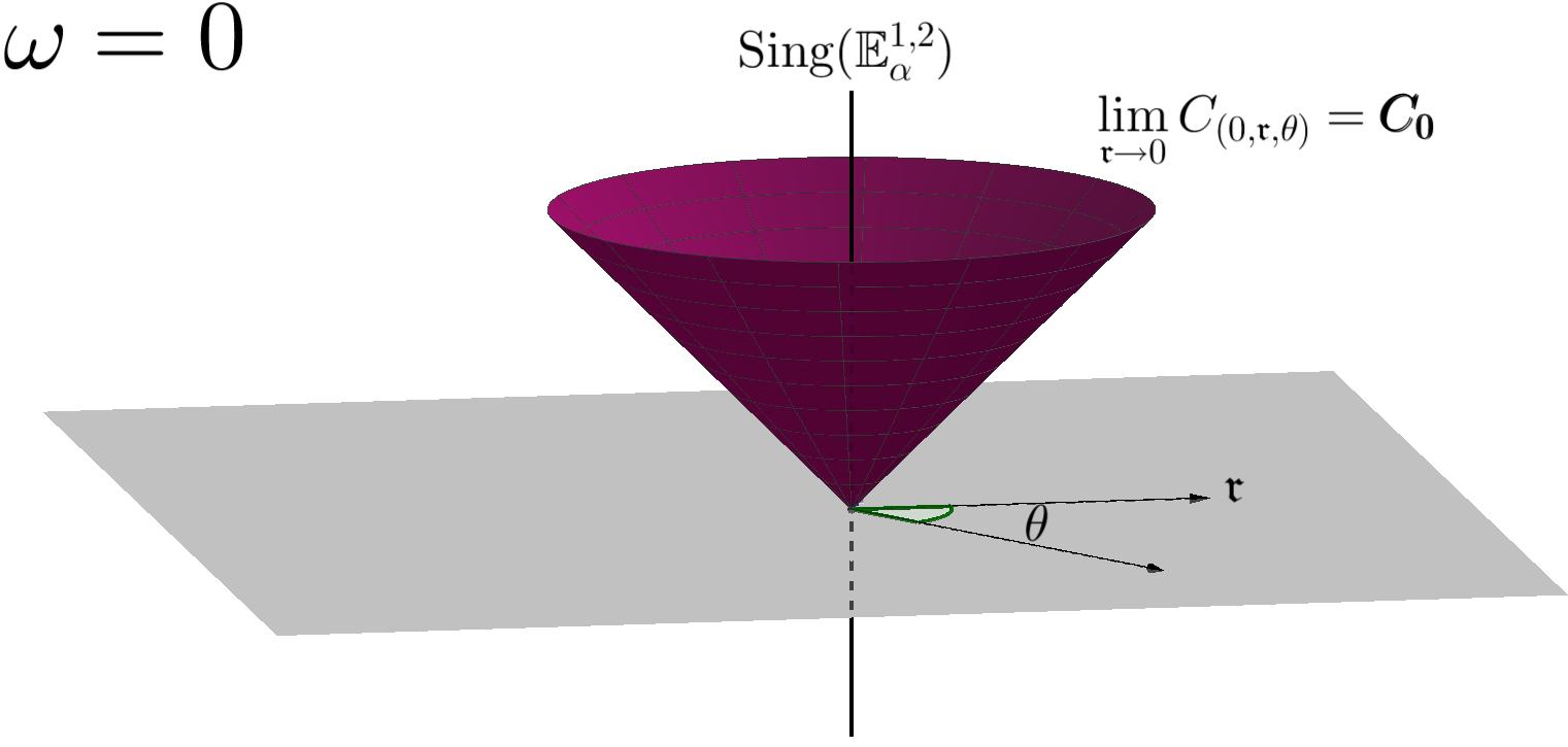
Figure 4: Futur Cones and limit futur cones in the tangent plane of a singular point.

We draw cones of future pointing causal vectors in $T_{p}\mathbb{E}^{1,2}_{\alpha}$ with $\alpha=2\pi\sqrt{1-\omega^{2}}$ and $p\in\mathrm{Sing}(\mathbb{E}^{1,2}_{\alpha})$ in the $(\tau,\mathfrak{r},\theta)$ coordinates. The red cone $C_{0}$ represents the cone of future pointing causal vectors at $p$ and the blue cone represents the radial limit toward $p$ of the cone of future pointing causal vectors. When $\omega=0$ (i.e. $\alpha=2\pi$), there the vertical line is not singular anymore and the red and blue cones blend.

It would be possible to construct a continous cone field wich contains the one of future causal vectors. Providing this new cone field is globally hyperbolic (in the sense of Fathi and Siconolfi) one could then apply the smoothing theorem and recover an everywhere smooth Cauchy-surface. This procedure might be slightly simpler and is much stronger since it allows to control both the position and the tangent plane of the Cauchy-surface. We didn’t write this here since we also needed Lemma 2.9 and we should have written the first two steps of the presented method anyway. Later on in this paper, we will need to control Cauchy-completeness of Cauchy-surfaces which presents, to our knowledge, the same difficulties using either Fathi-Siconolfi theorem or our method. Still, it would be nice to have an extended Fathi-Siconolfi theorem which directly applies. This would require to weaken the continuity hypothesis to some semi-continuity hypothesis which seems reasonable considering the methods they used.

3 Catching BTZ-lines : BTZ-extensions

In the example of the modular group presented in the Introduction, we added BTZ-lines to a Cauchy-maximal spacetime. Therefore, the usual Cauchy-maximal extension theorem doesn’t catch them. Since we want to add BTZ-lines to some given manifold whenever it is possible, we define BTZ-extensions and prove a corresponding maximal BTZ-extension theorem.

3.1 BTZ-extensions, definition and properties

Consider the regular part of $\mathbb{E}^{1,2}_{0}$. It is a Cauchy-maximal globally hyperbolic $\mathbb{E}^{1,2}$-manifold and should be naturally extended into $\mathbb{E}^{1,2}_{0}$. To get this we need new extensions. Let $A\subset\mathbb{R}_{+}$ be a subset containing $0$.

Definition 3.1 (BTZ-embedding, BTZ-extension).

Let $M_{1},M_{2}$ be two globally hyperbolic $\mathbb{E}^{1,2}_{A}$ manifolds and $\phi:M_{1}\rightarrow M_{2}$ a morphism of $\mathbb{E}^{1,2}_{A}$-structure. If $\phi$ is injective and the complement of its image in $M_{2}$ is a union (possibly empty) of BTZ lines then $\phi$ is a BTZ-embedding and $M_{2}$ is a BTZ-extension of $M_{1}$.

The following lemmas ensure that two BTZ lines cannot be joined via an extension and that the BTZ-lines cannot be completed in the future via BTZ-extensions.

Lemma 3.2.

Let $M_{1}$ and $M_{2}$ be two globally hyperbolic $\mathbb{E}^{1,2}_{A}$-manifolds, and $M_{1}\xrightarrow{\phi}M_{2}$ a BTZ extension. Let $p,q\in\mathrm{Sing}_{0}(M_{1})$, if $p$ and $q$ are in the same connected component of $\mathrm{Sing}_{0}(M_{2})$ then they are in the same connected component of $\mathrm{Sing}_{0}(M_{1})$.

Proof.

The connected component of $p$ in $\mathrm{Sing}_{0}(M_{2})$ is an inextendible causal curve we note $\Delta$. We may assume $p\in J^{-}_{M_{2}}(q)$. Since every point of $[p,q]$ is locally modeled on $\mathbb{E}^{1,2}_{0}$, we can construct a tube neighborhood of $[p,q]$ of some radius $R$. Take some regular point $q^{\prime}$ in the chronological future of $q$ in the tube neighborhood. The diamond $J^{-}_{M_{1}}(q^{\prime})\cap J^{+}_{M_{1}}(p)$ is compact, thus $[p,q]\subset\overline{I^{+}(p)\cap I^{-}(q^{\prime})}\subset J^{-}_{M_{1}}(q^{\prime})\cap J^{+}_{M_{1}}(p)\subset M_{1}$. ∎

Lemma 3.3.

Let $M_{1}$ and $M_{2}$ be two globally hyperbolic $\mathbb{E}^{1,2}_{A}$-manifolds, and $M_{1}\xrightarrow{\phi}M_{2}$ a BTZ extension. Let $p,q\in\mathrm{Sing}_{0}(M_{2})$. If $p\in J^{-}_{M_{2}}(q)$ and $p\in M_{1}$ then $q\in M_{1}$.

Proof.

Take some tube neighborhood $\mathcal{T}$ of radius $R$ of $[p,q]$. Take some point $q^{\prime}\in\left(\partial J^{+}_{M_{2}}(q)\right)\cap\mathcal{T}$ then $p\in I^{-}_{M_{2}}(q^{\prime})$. The diamond $\overline{\Diamond}_{p}^{q^{\prime}}$ in $M_{1}$ is compact and its interior is the open diamond $\Diamond_{p}^{q^{\prime}}$. The latter is relatively compact in $M_{2}$ and the former contains its closure in $M_{2}$ which contains $[p,q]$. Thus $[p,q]$ is in $M_{1}$. ∎

3.2 Maximal BTZ-extension theorem

We can now address the maximal BTZ-extension problem for globally hyperbolic $\mathbb{E}^{1,2}_{A}$-manifolds. More precisely, we prove the following theorem.

Theorem II (Maximal BTZ-extension).

Let $A\subset\mathbb{R}_{+}$, let $M$ be a globally hyperbolic $\mathbb{E}^{1,2}_{A}$-manifold. There exists a maximal BTZ-extension $\overline{M}$ of $M$. Furthermore it is unique up to isometry.

Again, we mean that a spacetime is BTZ-maximal if any BTZ-extension is surjective hence an isomophism. The proof has similarities with the one of the maximal Cauchy-extension theorem. Let $M$ a spacetime and consider two BTZ-embeddings $f:M_{0}\rightarrow M_{1}$ and $g:M_{0}\rightarrow M_{2}$.

Definition 3.4.

Define $M_{1}\wedge M_{2}$ the union of extensions $M$ of $M_{0}$ in $M_{1}$ such that there exists a BTZ-embedding $\phi_{M}:M\rightarrow M_{2}$ with $\phi_{M}\circ f=g$.

Definition 3.5 (Greatest common sub-extension).

Define

$$\phi:\begin{array}[]{l|rcl}&\displaystyle M_{1}\wedge M_{2}&\longrightarrow&\displaystyle M_{2}\\ &\displaystyle x&\longmapsto&\displaystyle\phi_{M}(x)\text{ if x}\in M\end{array}$$

This function $\phi$ is well defined since each $\phi_{M}$ is continuous and $f(M_{0})$ is dense in $M_{1}$.

Proposition 3.6.

$\phi$ is a BTZ-embedding.

Proof.

The image of $\phi$ contains the image of $M_{0}$ thus its complement in $M_{2}$ is a subset of $\mathrm{Sing}_{0}(M_{2})$. We must show $\phi$ is injective. Let $N_{1}$ and $N_{2}$ be two subextensions of $M_{1}$ together with BTZ-embeddings $\phi_{i}:N_{i}\rightarrow M_{2}$. Let $(x,y)\in N_{1}\cup N_{2}$ be such that $\phi(x)=\phi(y)=p\in M_{2}$. Notice that $I^{+}(p)\subset M_{2}\setminus\mathrm{Sing}_{0}(M_{2})$ thus

$$\emptyset\neq I^{+}(p)=\phi_{1}(I^{+}(x))=\phi_{2}(I^{+}(y))\subset g(M_{0}).$$

Then $I^{+}(x)=f\circ g^{-1}(I^{+}(p))=I^{+}(y)$ and $x=y$. ∎

Definition 3.7 (Least common extension).

Define the least common extension of $M_{1}$ and $M_{2}$ :

$$M_{1}\vee M_{2}=(M_{1}\coprod M_{2})/(M_{1}\wedge M_{2})$$

where the quotient is understood identifying $M_{1}\wedge M_{2}$ and $\phi(M_{1}\wedge M_{2})$. The define the natural projetction

$$\pi:M_{1}\coprod M_{2}\rightarrow M_{1}\vee M_{2}.$$

The following diagram sums-up the situation.

Notice that $M_{1}\vee M_{2}$ need not be Hausdorff. There could be non spearated points, i.e. points $p,q$ such that for every couple of open neighborhoods $(\mathcal{U},\mathcal{V})$ of $p$ and $q$, $\mathcal{U}\cap\mathcal{V}\neq\emptyset$.

Definition 3.8.

Define $C=\{p\in M_{1}\wedge M_{2}\leavevmode\nobreak\ |\leavevmode\nobreak\ \pi(p)\text{ is not separated}\}$

The following Propositions prove that $(M_{1}\wedge M_{2})\cup C$ is a globally hyperbolic $\mathbb{E}^{1,2}_{A}$-manifold to which $\phi$ extends. Thus it is a sub-BTZ-extension common to $M_{1}$ and $M_{2}$. It will prove that $C=\emptyset$.

Proposition 3.9.

$(M_{1}\wedge M_{2})\cup C$ is open and $\phi$ extends injectively to $(M_{1}\wedge M_{2})\cup C$.

Proof.

Since $M_{1}\wedge M_{2}$ is a $\mathbb{E}^{1,2}_{A}$-manifold we shall only check the existence of a chart around points of $C$. The set $C$ is in the complement of $M_{1}\wedge M_{2}$ and thus is a subset of $\mathrm{Sing}_{0}(M_{1})$. Let $p\in C$ and $p^{\prime}\in M_{2}$ such that $\pi(p)$ and $\pi(p^{\prime})$ are not separated in $M_{1}\vee M_{2}$. Let $\mathcal{U}_{p}\xrightarrow{\psi_{p}}\mathcal{V}_{p}\subset\mathbb{E}^{1,2}_{0}$ a chart around $p$ and $\mathcal{U}_{p^{\prime}}\xrightarrow{\psi_{p^{\prime}}}\mathcal{V}_{p^{\prime}}\subset\mathbb{E}^{1,2}_{\alpha}$ a chart around $p^{\prime}$. Since $\pi(p)$ and $\pi(p^{\prime})$ are not separated, there exists a sequence $(p_{n})_{n\in\mathbb{N}}\in Reg(M_{1})^{\mathbb{N}}$ such that $\lim_{n\rightarrow+\infty}p_{n}=p$ and $\lim_{n\rightarrow+\infty}\phi(p_{n})=p^{\prime}$. Take such a sequence, notice that forall $n\in\mathbb{N}$, $\phi(I^{+}(p_{n}))=I^{+}(\phi(p_{n}))$ and that $I^{+}(p)\subset\bigcup_{n\in\mathbb{N}}I^{+}(p_{n})$ and $I^{+}(p^{\prime})\subset\bigcup_{n\in\mathbb{N}}I^{+}(\phi(p_{n}))$. We then get $\phi(I^{+}(p))=I^{+}(p^{\prime})$. Therefore, taking smaller $\mathcal{U}_{p}$ and $\mathcal{U}_{p^{\prime}}$ if necessary, we may assume, $\mathcal{U}_{p}$ connected and $\phi(I^{+}(p)\cap\mathcal{U}_{p})=I^{+}(p^{\prime})\cap\mathcal{U}_{p^{\prime}}$ then

$$\psi_{p^{\prime}}\circ\phi\circ\psi_{p}^{-1}:I^{+}(\psi_{p}(p))\cap\mathcal{V}_{p}\rightarrow I^{+}(\psi_{p^{\prime}}(p^{\prime}))\cap\mathcal{V}_{p^{\prime}}$$

is an injective $\mathbb{E}^{1,2}$-morphism. The future of a point in $\mathcal{V}_{p}$ is the regular part of a neighborhood of some piece of the singular line in $\mathbb{E}^{1,2}_{0}$. Thus, by Proposition 1.19, $\alpha=0$ and $\psi_{p^{\prime}}\circ\phi\circ\psi_{p}^{-1}$ is the restriction of an isomophism of $\mathbb{E}^{1,2}_{0}$ say $\gamma_{p}$. Choose such neighborhood $\mathcal{U}_{p}$, such $\psi_{p},\psi_{p^{\prime}}$ and such $\gamma_{p}$ for all $p\in C$. The subset $(M_{1}\wedge M_{2})\cup\bigcup_{p\in C}\mathcal{U}_{p}$ is open thus a $\mathbb{E}^{1,2}_{A}$-manifold and the $\mathbb{E}^{1,2}_{A}$-morphism

$$\overline{\phi}:\begin{array}[]{l|rcl}&\displaystyle(M_{1}\wedge M_{2})\cup\bigcup_{p\in C}\mathcal{U}_{p}&\longrightarrow&\displaystyle M_{2}\\ &\displaystyle x&\longmapsto&\displaystyle\left\{\begin{array}[]{ll}\phi(x)&\text{ if }x\in M_{1}\wedge M_{2}\\ \psi_{p^{\prime}}^{-1}\circ\gamma\circ\psi_{p}(x)&\text{ if }x\in\mathcal{U}_{p}\end{array}\right.\end{array}$$

is then well defined by Lemma 1.24. Notice that for all $p\in C$ and all $q\in\mathrm{Sing}_{0}(\mathcal{U}_{p})$, the points $\pi(q)$ and $\pi\circ\overline{\phi}(q)$ of $M_{1}\vee M_{2}$ are not separated. Therefore, either $q\in C$ or $\pi(q)=\pi\circ\overline{\phi}(q)$ thus

$$(M_{1}\wedge M_{2})\cup\bigcup_{p\in C}\mathcal{U}_{p}=(M_{1}\wedge M_{2})\cup C$$

and thus $(M_{1}\wedge M_{2})\cup C$ is open. It remains to show that $\overline{\phi}$ is injective. If $p,q\in(M_{1}\wedge M_{2})\cup C$ have same image by $\overline{\phi}$ then the image by $\overline{\phi}$ of any neighborhood of $p$ intersects the image of any neighborhood of $q$. This intersection is open and thus contains regular points. We can construct sequences of regular points $p_{n}\rightarrow p$ and $q_{n}\rightarrow q$ such that $\phi(p_{n})=\phi(q_{n})$. By injectivity of $\phi$, $\forall n\in\mathbb{N},p_{n}=q_{n}$ and thus, since $M_{1}$ is Hausdorff, $p=q$. ∎

Proposition 3.10.

$(M_{1}\wedge M_{2})\cup C$ is globally hyperbolic.

Proof.

Write $M=(M_{1}\wedge M_{2})\cup C$ and let $p,q\in M$, we now show that $J^{-}_{M}(q)\cap J^{+}_{M}(p)$ is compact. We identify $M_{0}$ and $f(M_{0})\subset M_{1}$. If $p\notin\mathrm{Sing}_{0}(M_{1})$, $J^{+}(p)\subset M\setminus\mathrm{Sing}_{0}(M_{1})\subset M_{0}$ and $J^{-}_{M}(q)\cap J^{+}_{M}(p)=J^{-}_{M_{0}}(q)\cap J^{+}_{M_{0}}(p)$ which is compact. Assume now $p$ is of type $\mathbb{E}^{1,2}_{0}$. Let $(x_{n})\in M^{\mathbb{N}}$ be sequence such that $\forall n\in\mathbb{N},x_{n}\in J^{+}_{M}(p)\cap J^{-}_{M}(q)$. By compactness of $J^{+}_{M_{1}}(p)\cap J^{-}_{M_{1}}(q)$, we can assume $(x_{n})$ converges to some $x\in\mathrm{Sing}_{0}(M_{1})$. Consider some compact tube slice neighborhood $\mathcal{T}$ of $[p,x]$ in $M_{1}$, the subset $M\cap[p,x]$ is open in $[p,x]$ and contains $p$. Consider $I=\{y\in[p,x]\leavevmode\nobreak\ |\leavevmode\nobreak\ [p,y]\subset M\}$. The set $I$ is connected and open in $[p,x]$. Take an increasing sequence $(y_{n})_{n\in\mathbb{N}}\in I^{\mathbb{N}}$, it converges toward some $y_{\infty}\in[p,x]$. Take some compact diamond neighborhood $\overline{\Diamond}_{p}^{p^{\prime}}$ of $]p,y_{\infty}[$ inside $\mathcal{T}$. We can take $p^{\prime}\in\partial J^{+}(y_{\infty})$ so that $p^{\prime}\in M_{0}\cap\mathcal{T}$. The diamond $\phi(\Diamond_{p}^{p^{\prime}})$ of $M_{2}$ is relatively compact thus one can extract a converging subsequence of $\phi(y_{n})$ toward some $y^{\prime}_{\infty}\in M_{2}$. Therefore $\pi(y^{\prime}_{\infty})$ and $\pi(y_{\infty})$ are not separated and $y_{\infty}\in M$. Finally, $M\cap[p,x]$ is closed and $I=[p,x]$. Finally, $x\in M$, the sequence $(x_{n})_{n\in\mathbb{N}}$ has a converging subsequence in $J^{+}_{M}(p)\cap J^{-}_{M}(q)$. ∎

Corollary 3.11.

$M_{1}\vee M_{2}$ is Hausdorff.

Proof.

$(M_{1}\wedge M_{2})\cup C$ is a BTZ-extension of $M_{0}$ inside $M_{1}$ with a BTZ-embedding into $M_{2}$. Therefore it is a subset of $M_{1}\wedge M_{2}$ by maximality of $M_{1}\wedge M_{2}$. Finally, $C=\emptyset$. ∎

The construction above of a least common extension show that the family of BTZ-extensions of $M_{0}$ is a right filtered family and can thus take the direct limit of all such extensions. Consider a family of representants of the isomorphism classes $(M_{i})_{i\in I}$ together with BTZ-embeddings $\phi_{ij}:M_{i}\rightarrow M_{j}$ whenever it exists. The direct limit of this family is

$$\overline{M}_{0}=\varinjlim_{i\in I}M_{i}=\left(\coprod_{i\in I}M_{i}\right)/\sim$$

where $x\sim y\Leftrightarrow\exists(i,j),\phi_{ij}(x)=y$. It remains to check that the topology of such a limit is second countable. The proof is an adaptation of the arguments of Geroch given in [Ger68].

3.3 A remarks on Cauchy and BTZ-extensions

One may ask what happens if one takes the Cauchy-extension then the BTZ-extension. Is the resulting manifold Cauchy-maximal? The answer is no as the following example shows.

Example 3.12.

Let $M_{0}=\{\tau<0,r>0\}$ be the past half tube in cylindrical coordinates of $\mathbb{E}^{1,2}_{0}$ and let $p=(\tau=0,r=0)$. The spacetime be $M_{0}$ is regular and globally hyperbolic. Let $M_{1}$ be its maximal Cauchy-extension, $M_{2}$ the maximal BTZ-extension of $M_{1}$ and $M_{3}$ the maximal Cauchy-extension of $M_{2}$.

• $M_{0}=Reg(\mathbb{E}^{1,2}_{0})\setminus J^{+}(\{\tau=0\})$

• $M_{1}=Reg(\mathbb{E}^{1,2}_{0})\setminus J^{+}(p)$.

• $M_{2}=\mathbb{E}^{1,2}_{0}\setminus J^{+}(p)$

• $M_{3}=\mathbb{E}^{1,2}_{0}$

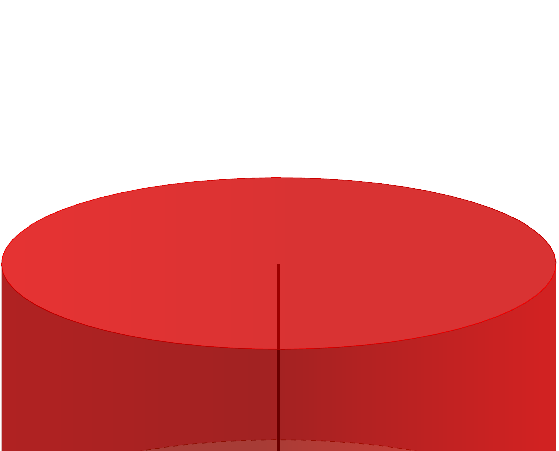
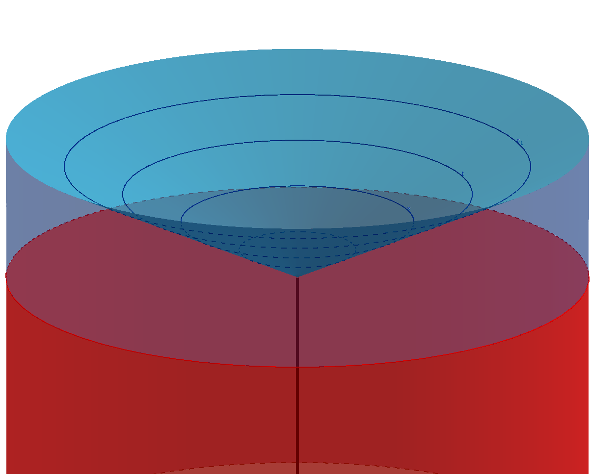
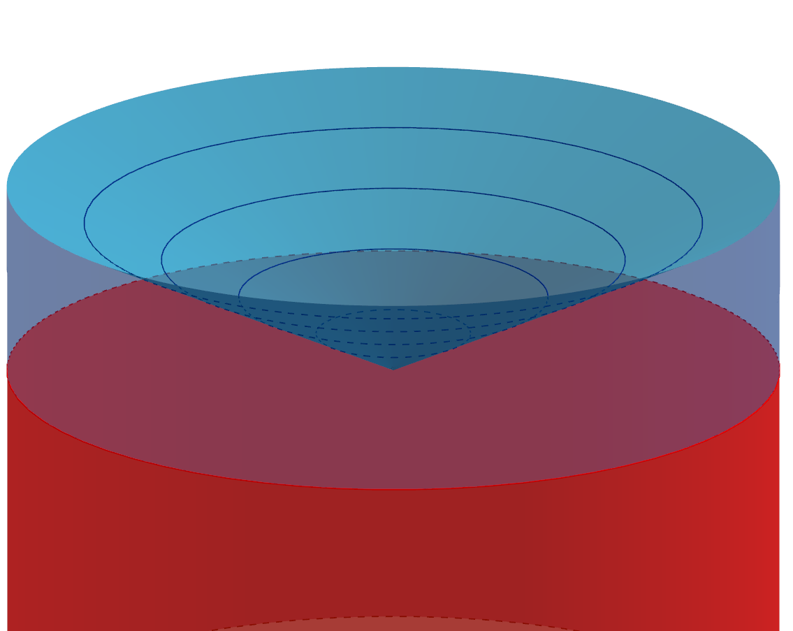
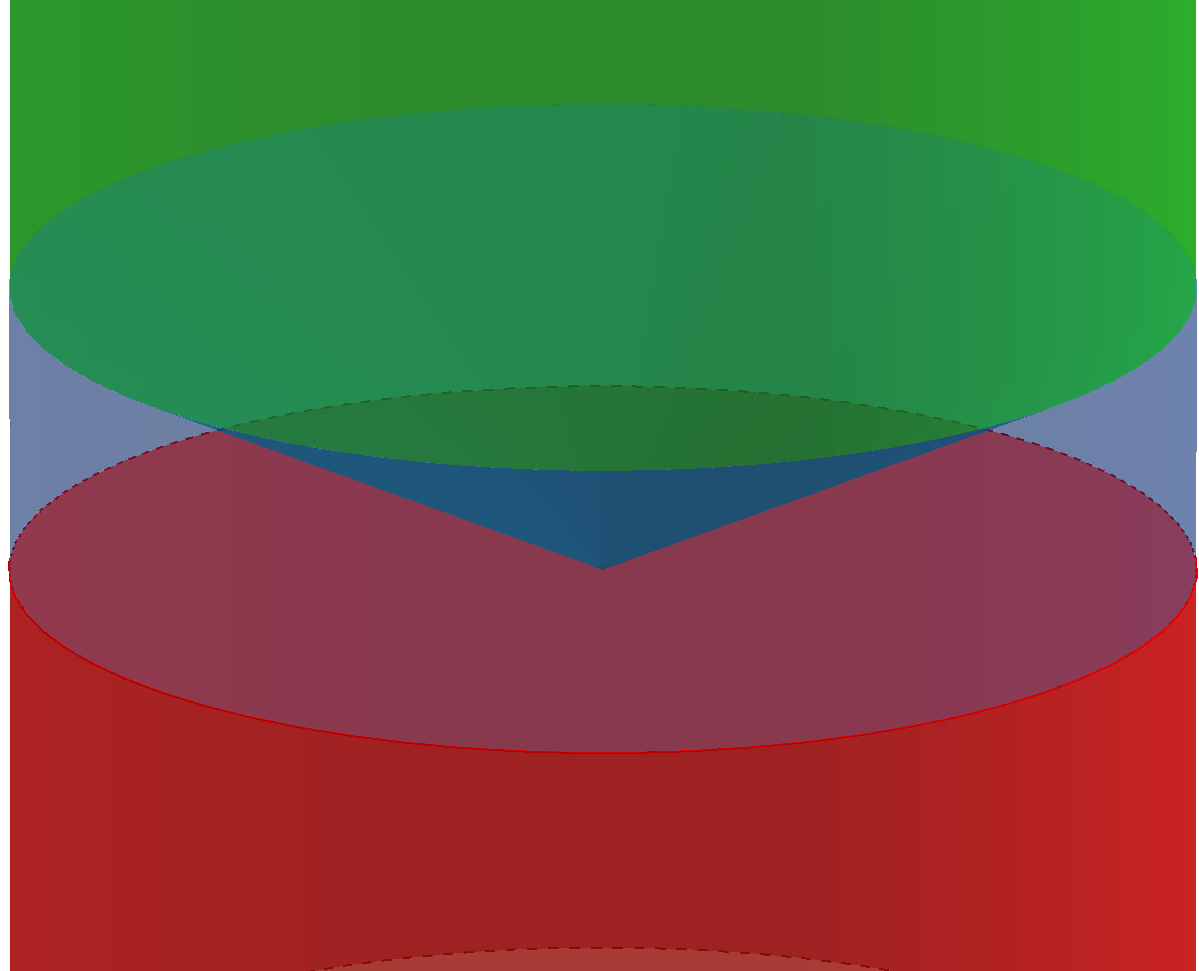
Figure 5: Successive maximal Cauchy-extension and BTZ-extension of a past half tube in ${\mathbb{E}_{0}^{1,2}}$.

In red the initial half tube, in black the BTZ line missing. In blue its Cauchy-extension then the BTZ line is caught via the BTZ-extension. In green the final Cauchy-extension

Conjecture 1.

Let $M_{0}$ be a globally hyperbolic singular manifold, $M_{1}$ its maximal Cauchy-extension, $M_{2}$ the maximal BTZ-extension of $M_{1}$, $M_{3}$ the maximal Cauchy-extension of $M_{2}$. Then $M_{3}$ is both Cauchy-maximal and BTZ-maximal.

4 Cauchy-completeness and extensions of spacetimes

Is the Cauchy-completeness of a space-time equivalent to the Cauchy-completeness of the maximal BTZ-extension ? The answer is yes and the whole section is devoted to the proof of this answer. We then aim at proving the following theorem.

Theorem III (Cauchy-completeness Conservation).

Let $M$ be a globally hyperbolic $\mathbb{E}^{1,2}_{A}$-manifold without BTZ point, the following are equivalent.

1. $M$ is Cauchy-complete and Cauchy-maximal.

2. There exists a Cauchy-complete and Cauchy-maximal BTZ-extension of $M$.

3. The maximal BTZ-extension of $M$ is Cauchy-complete and Cauchy-maximal.

The proof decomposes into four parts. When taking a BTZ-extension, the Cauchy-surface changes. The proof of the theorem needs to modify Cauchy-surfaces in a controlled fashion. The first part is devoted to some lemmas useful to construct good spacelike surfaces. The other two parts solve the causal issues proving that the surfaces constructed using the first part are indeed Cauchy-surfaces. Pieces are put together in the fourth part to prove the theorem.

4.1 Surgery of Cauchy-surfaces around a BTZ-line

We begin by an example illustrating the situation we will soon manage.

Example 4.1.

Consider $\mathbb{E}^{1,2}_{0}$ endowed with its coordinates $(\tau,r,\theta)$ and the Cauchy-surface $\Sigma:=\{\tau=1\}$. The regular part of $\Sigma$, $\Sigma^{*}:=Reg(\Sigma)$, is not a Cauchy-surface of the regular part of $\mathbb{E}^{1,2}_{0}$ since its Cauchy development is $Reg(\mathbb{E}^{1,2}_{0})\setminus J^{+}(\{\tau=1,r=0\})$. The problem is that a curve such as $\{\tau=2r+\tau_{0},\theta=\theta_{0}\}$ is causal, inextendible in $Reg({\mathbb{E}_{0}^{1,2}})$ and doesn’t intersects $\Sigma^{*}$ for $\tau_{0}>0$. A solution consists in noticing that $\Sigma^{*}$ coincides with $\mathbb{H}^{2}_{0}:=\left\{\tau=\frac{1+r^{2}}{2r}\right\}$ on $\{r=1,\tau=1\}$. Therefore, we can glue the piece of $\mathbb{H}^{2}_{0}$ inside the tube of radius 1 with the plane $\{\tau=1\}$ outside the tube of radius 1 and get a complete Cauchy-surface $\Sigma_{1}$ of the regular part of $\mathbb{E}^{1,2}_{0}$. See figure 6 below.

A)	B)

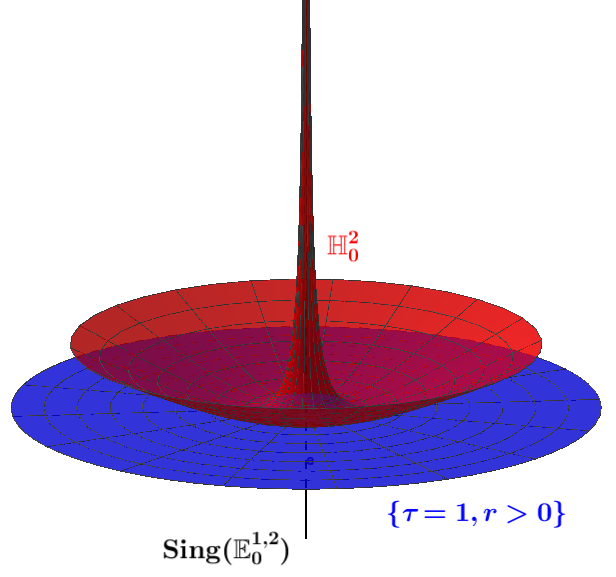
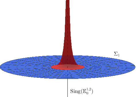
Figure 6: Two acausal surfaces, the boundary of their Cauchy development, two different gluings.

1. The blue plane represents the surface $\Sigma^{*}=\{\tau=1,r>0\}$ and the red surface is $\mathbb{H}_{0}^{2}$.

2. The gluing $\Sigma_{1}$ of $\mathbb{H}^{2}_{0}\cap\{r\leq 1\}$ with $\Sigma^{*}\cap\{r\geq 1\}$. It is a Cauchy-surface of ${\mathbb{E}_{0}^{1,2}}$.

Let $M$ be a Cauchy-complete spacetime. Starting from a complete Cauchy-surface $\Sigma$ of $M$, we need construct a complete Cauchy-surface of $M\setminus\Delta$ where $\Delta$ is a BTZ line. This is done locally around the singular line : the intersection of $\Sigma$ with the boundary of a tube neighborhood of $\Delta$ gives a curves and the second point of the main Lemma 4.3 below show that such a curve can be extended to a complete surface avoiding the singular line of $\mathbb{E}^{1,2}_{0}$. This procedure is the heart of the proof of $(ii)\Rightarrow(i)$ in Theorem III. To obtain $(i)\Rightarrow(iii)$, half of the work consists in doing the opposite task. Let $M$ be a Cauchy-complete spacetime. Starting from a complete Cauchy-surface of $M$, we construct a complete Cauchy-surface of its maximal BTZ extension by modifying locally a Cauchy-surface of $M$ around a singular line. We start from the intersection of the Cauchy-surface of $M$ along the boundary of a tube around a singular line, this gives us a curve on a boundary of a tube in $\mathbb{E}^{1,2}_{0}$. The first point of the main Lemma 4.3 below show that such a curve can be extended to a complete surface which cuts the singular line of $\mathbb{E}^{1,2}_{0}$.

Definition 4.2.

Define $\mathbb{D}_{R}$ the Euclidean disc of radius $R>0$ and $\mathbb{D}_{R}^{*}$ the punctured Euclidean disc of radius $R>0$. We identify frequently $\mathbb{D}_{R}$ with its embedding in $\{\tau=0,r\leq R\}$.

Lemma 4.3.

Let $\mathcal{T}$ be a closed future half-tube in $\mathbb{E}^{1,2}_{0}$ of radius $R$ and let $\tau_{\Sigma}^{R}:\partial\mathbb{D}_{R}\rightarrow\mathbb{R}_{+}$ be a smooth function. Then

1. there exists a piecewise smooth function $\tau_{\Sigma}:\mathbb{D}_{R}\rightarrow\mathbb{R}_{+}$ extending $\tau_{\Sigma}^{R}$ which graph is acausal, spacelike and complete;

2. there exists a piecewise smooth function $\tau_{\Sigma}:\mathbb{D}_{R}^{*}\rightarrow\mathbb{R}_{+}$ extending $\tau_{\Sigma}^{R}$ which graph is acausal, spacelike and complete.

Before proving Lemma 4.3, we need to do some local analysis in a tube of $\mathbb{E}^{1,2}_{0}$. We begin by a local condition for acausality.

Lemma 4.4.

Let $R>0$ and let $\mathcal{T}:=\{\tau>0,r\leq R\}$ be a closed future half tube in ${\mathbb{E}_{0}^{1,2}}$ of radius $R$ in cylindrical coordinates. Let $\tau_{\Sigma}\in\mathscr{C}^{1}(]0,R]\times\mathbb{R}/2\pi\mathbb{Z},\mathbb{R}_{+}^{*})$ and $\Sigma=\mathrm{Graph}(\tau_{\Sigma})=\{(\tau_{\Sigma}(r,\theta),r,\theta):(r,\theta)\in\mathbb{D}^{*}\}$, then $(i)\Leftrightarrow(ii)\Leftrightarrow(iii)$.

1. $\Sigma$ is spacelike and acausal

2. $\Sigma$ is spacelike

3. $\displaystyle 1-2\frac{\partial\tau_{\Sigma}}{\partial r}-\left(\frac{1}{r}\frac{\partial\tau_{\Sigma}}{\partial\theta}\right)^{2}>0$

Proof.

Beware that spacelike is a local condition but acausal is a global one. The implication $(i)\Rightarrow(ii)$ is obvious. Writing $\delta=\left(1-2\frac{\partial\tau_{\Sigma}}{\partial r}-\left(\frac{1}{r}\frac{\partial\tau_{\Sigma}}{\partial\theta}\right)^{2}\right)$ from direct computations :

$$\mathrm{d}s_{\Sigma}^{2}=\delta\mathrm{d}r^{2}+\left(\frac{1}{r}\frac{\partial\tau_{\Sigma}}{\partial\theta}\mathrm{d}r-r\mathrm{d}\theta\right)^{2}.$$

and let $c(s)=\tau_{\Sigma}(r(s),\theta(s)),s\in]s_{*},s^{*}[$ be some path on $\Sigma$, then :

$$\frac{\mathrm{d}s_{c}^{2}}{\mathrm{d}s^{2}}=(r^{\prime})^{2}\delta(s)+\left(\frac{\partial\tau_{\Sigma}}{\partial\theta}\frac{r^{\prime}}{r}-r\theta^{\prime}\right)^{2}$$

$\Sigma$ is spacelike iff its Riemann metric is postive definite iff $\delta>0$ thus $(ii)\Leftrightarrow(iii)$. To prove $(iii)\Rightarrow(i)$ take a smooth future causal curve $c=(\tau,r,\theta)$ such that $c(0)\in\Sigma$, i.e. $\tau_{\Sigma}(r(0),\theta(0))=\tau(0)$. Since $\tau^{\prime}$ is increasing, reparametrizing $c$ if necessary, we can assume $\tau^{\prime}>0$. Let $f:s\mapsto\tau(s)-\tau_{\Sigma}(r(s),\theta(s))$ so that $f(s)=0$ if and only if $c(s)\in\Sigma$, notice $f(0)=0$. On the one hand, since $c$ is causal, we have

$$r^{\prime}\geq 0\quad\text{and}\quad 2\tau^{\prime}(s)r^{\prime}(s)\geq(r^{\prime})^{2}+r^{2}(\theta^{\prime})^{2}.$$

On the other hand, using $\delta>0$, if $r^{\prime}>0$

$$2\left(\frac{\mathrm{d}}{\mathrm{d}s}\tau_{\Sigma}(r,\theta)\right)r^{\prime} = 2\left(\frac{\partial\tau_{\Sigma}}{\partial\theta}\theta^{\prime}+\frac{\partial\tau_{\Sigma}}{\partial r}r^{\prime}\right)r^{\prime}$$ (7)

$$< 2\frac{\partial\tau_{\Sigma}}{\partial\theta}\theta^{\prime}r^{\prime}+(r^{\prime})^{2}-\left(\frac{r^{\prime}}{r}\frac{\partial\tau_{\Sigma}}{\partial\theta}\right)^{2}$$ (8)

$$\leq -\frac{\left(2\theta^{\prime}r^{\prime}\right)^{2}-4\left(-\frac{(r^{\prime})^{2}}{r^{2}}\right)(r^{\prime})^{2}}{-4\frac{(r^{\prime})^{2}}{r^{2}}}$$ (9)

$$= r^{2}(\theta^{\prime})^{2}+(r^{\prime})^{2}.$$ (10)

Let $s\in\mathbb{R}$, if $r^{\prime}(s)>0$ then the computation above shows $f^{\prime}(s)>0$. If $r^{\prime}(s)=0$ then $\theta^{\prime}(s)=0$ thus $f^{\prime}(s)=\tau^{\prime}(s)>0$. Thus $f$ is increasing, thus injective. Finally $f$ cannot be naught twice and $c$ cannot intersect $\Sigma$ twice. $\Sigma$ is thus acausal. ∎

Lemma 4.5 (Completeness criteria).

Using the same notation as in Lemma 4.4 we have :

1. $\Sigma$ is spacelike and complete if
   $\exists C>0,\forall(r,\theta)\in\mathbb{D}_{R}^{*},$

   $$1-2\frac{\partial\tau_{\Sigma}}{\partial r}-\left(\frac{1}{r}\frac{\partial\tau_{\Sigma}}{\partial\theta}\right)^{2}\geq\frac{C^{2}}{r^{2}}$$

   Furthermore, in this case the Cauchy development of $\Sigma$ is $\mathcal{T}\setminus\Delta$.

2. If $\Sigma$ is spacelike and complete then,

   $$\lim_{(r,\theta)\rightarrow 0}\tau_{\Sigma}(r,\theta)=+\infty$$

Proof.

We use the same notations as in the proof of Lemma 4.4. We insist on the fact that $\mathcal{T}$ is closed, which means for instance that $\Sigma$ has a boundary parametrised by $\partial\mathbb{D}_{R}$. It also means that a curve ending on the boundary of $\mathcal{T}$ can be extended since it has an ending point.

1. Let $C>0$ be such as $\delta>\frac{C^{2}}{r^{2}}$. It suffice to prove that a finite length curve in $\Sigma$ is extendible. Let $\gamma:\mathbb{R}\rightarrow\Sigma$ be a finite length piecewise smooth curve on $\Sigma$. Write $\gamma(s)=(\tau_{\Sigma}(r(s),\theta(s)),r(s),\theta(s))$ for $s\in\mathbb{R}$ and $l(\gamma)$ its length. Since $l(\gamma)\geq\int_{\mathbb{R}}|r^{\prime}(s)|\frac{C}{R}\mathrm{d}s$ and $l(\gamma)<+\infty$, then $r^{\prime}\in\mathrm{L}^{1}$ and $r$ converges as $s\rightarrow+\infty$, let $r_{\infty}:=\lim_{s\rightarrow+\infty}r(s)$. For all $a\in\mathbb{R}$, $l(\gamma)\geq\left|\int_{0}^{a}\frac{C|r^{\prime}(s)|}{r(s)}\mathrm{d}s\right|\geq C\left|\ln\left(\frac{r(0)}{r(a)}\right)\right|$. Thus

   $$\forall a\in\mathbb{R},\leavevmode\nobreak\ \leavevmode\nobreak\ r(a)\geq r(0)e^{-\frac{1}{C}l(\gamma)}>0$$

   and thus $r_{\infty}>0$. Take $A>0$ such as $\forall s\geq A,r(s)\in[r_{*},r^{*}]$ with $r_{*}=r_{\infty}/2$ and $r^{*}=(r_{\infty}+R)/2$ then for all $b\geq a\geq A$ :

   $$l(\gamma) \geq \int_{[a,b]}r\left|\frac{\partial\tau}{\partial\theta}\frac{r^{\prime}}{r^{2}}-\theta^{\prime}\right|$$ (11)

   $$\geq \int_{[a,b]}r_{*}\left|\frac{\partial\tau}{\partial\theta}\frac{r^{\prime}}{r^{2}}-\theta^{\prime}\right|$$ (12)

   $$\geq \int_{[a,b]}r_{*}\left(\left|\theta^{\prime}\right|-\left|\frac{\partial\tau}{\partial\theta}\frac{r^{\prime}}{r^{2}}\right|\right)$$ (13)

   $$\geq r_{*}\int_{[a,b]}\left|\theta^{\prime}\right|-r_{*}\left(\max_{(r,\theta)\in[r_{*},r^{*}]\times\mathbb{R}/2\pi\mathbb{Z}}\left|\frac{\partial\tau}{\partial\theta}\right|\right)\ \int_{[a,b]}\left|\frac{r^{\prime}}{r^{2}}\right|$$ (14)

   By integration by part, noting $F$ a primitive of $|r^{\prime}|$, and for some constant $C^{\prime}>0$.

   $$l(\gamma)\geq r_{*}\int_{[a,b]}\left|\theta^{\prime}\right|-C^{\prime}\left(\left[\frac{F}{r^{2}}\right]_{a}^{b}+2\int_{a}^{b}\frac{Fr^{\prime}}{r^{3}}\right)$$

   Since $\int_{\mathbb{R}}|r^{\prime}|<+\infty$, $F$ is bounded and can be chosen positive. Set $B=\sup_{s\in\mathbb{R}}R(s)$, thus for some $C^{\prime\prime},C^{\prime\prime\prime}>0$,

   $$\forall b>A,\leavevmode\nobreak\ \leavevmode\nobreak\ \leavevmode\nobreak\ l(\gamma)+C^{\prime\prime}\geq C^{\prime\prime\prime}\int_{[a,b]}|\theta^{\prime}|$$

   Which proves that $\int_{[a,+\infty[}|\theta^{\prime}|\mathrm{d}s<+\infty$, so that $\theta(s)$ converges as $s\rightarrow+\infty$. Consequently, $\tau(r,\theta)$ converges in $\Sigma$. Since $\mathcal{T}$ is closed, the curve $\gamma$ is then extendible. We conclude that $\Sigma$ is complete.
    
   Let $c=(\tau_{c},r_{c},\theta_{c}):\mathbb{R}\rightarrow\mathcal{T}\setminus\Delta$ be an inextendible future oriented causal curve. We must show that $c$ intersects $\Sigma$. Since $c$ is future oriented, $\tau_{c}$ is increasing and $r_{c}$ is non-decreasing. Both functions have then limits at $\pm\infty$. Let $r^{*}=\lim_{s\rightarrow+\infty}r_{c}(s)$, $r_{*}=\lim_{s\rightarrow-\infty}r_{c}(s)$, $\tau_{*}=\lim_{s\rightarrow-\infty}\tau_{c}(s)$ and $\tau^{*}=\lim_{s\rightarrow+\infty}\tau_{c}(s)$. Since $r_{c}$ is non-decreasing, $r^{*}>0$ and since $\tau_{c}$ is increasing, $\tau^{\prime}_{c}>0$. Assume $\tau^{*}<\infty$, then $\tau^{\prime}_{c}\in L^{1}([0,\infty[)$. We have on $[0,+\infty[$:

   $$(r_{c}^{\prime})^{2}+r_{c}^{2}(\theta^{\prime})^{2}-2r_{c}^{\prime}\tau_{c}^{\prime} \leq 0$$ (15)

   $$(\theta^{\prime})^{2} \leq \frac{(\tau_{c}^{\prime})^{2}-(\tau_{c}^{\prime}-r_{c}^{\prime})^{2}}{r_{c}^{2}}$$ (16)

   $$|\theta^{\prime}| \leq \frac{1}{r_{c}(0)}\tau_{c}^{\prime}$$ (17)

   Thus $\theta^{\prime}\in\mathrm{L}^{1}([0,+\infty[)$ and $\theta$ has a limit at $+\infty$. The same way, we have :

   $$|r_{c}^{\prime}-\tau^{\prime}_{c}|\leq\tau_{c}^{\prime}$$

   Thus $(r_{c}^{\prime}-\tau_{c}^{\prime})\in L^{1}([0,\infty[)$ and so is $r^{\prime}_{c}$. Since $r$ has a non zero limit at $+\infty$ and $\mathcal{T}$ is closed, $c$ is extendible ; therefore, $\tau^{*}=+\infty$. Since $r^{*}\in]0,R]$ and since $\tau^{*}=+\infty$,

   $$\exists s_{0}\in\mathbb{R},\forall s>s_{0},\leavevmode\nobreak\ \leavevmode\nobreak\ \tau_{c}(s)>\left(\max_{[r^{*}/2,r^{*}]\times\mathbb{R}/2\pi\mathbb{Z}}\tau_{\Sigma}\right)\geq\tau_{\Sigma}(r_{c}(s),\theta_{c}(s))$$

   Similar arguments can be used to prove that either $\tau_{*}=0$ or $r_{*}=0$. Furthermore, one may check that the assumption implies that $\lim_{r\rightarrow 0}\left(\min_{\theta\in\mathbb{R}/2\pi\mathbb{Z}}\tau_{\Sigma}(r,\theta)\right)=+\infty$. This implies that $\min\tau_{\Sigma}>0$. Assume $\tau_{*}=0$, since $\min\tau_{\Sigma}>0$, we have :

   $$\exists s_{0}\in\mathbb{R},\forall s<s_{0},\leavevmode\nobreak\ \leavevmode\nobreak\ \tau_{c}(s)<\min\tau_{\Sigma}\leq\tau_{\Sigma}(r_{c}(s),\theta_{c}(s))$$

   If on the contrary we assume $\tau_{*}>0$ and $r_{*}=0$ then

   $$\exists r\in\mathbb{R}_{+}^{*},\min_{]0,r]\times\mathbb{R}/2\pi\mathbb{Z}}\tau_{\Sigma}>\tau_{*}$$

   For such an $r\in\mathbb{R}_{+}^{*}$,

   $$\exists s_{0}\in\mathbb{R},\forall s<s_{0},\leavevmode\nobreak\ \leavevmode\nobreak\ \tau_{c}(s)<\tau_{\Sigma}(r_{c}(s),\theta_{c}(s))$$

   In any case, by continuity, there exists $s\in\mathbb{R}$ such that $\tau_{c}(s)=\tau(r_{c}(s),\theta_{c}(s))$ and thus such that $c(s)\in\Sigma$.

2. Since $\Sigma$ is spacelike the point $(ii)$ of Lemma 4.4 ensures that

   $$1-2\frac{\partial\tau_{\Sigma}}{\partial r}-\left(\frac{1}{r}\frac{\partial\tau_{\Sigma}}{\partial\theta}\right)^{2}\geq 0$$

   on $]0,R]\times\mathbb{R}/2\pi\mathbb{Z}$. Consider a sequence $(r_{n},\theta_{n})\rightarrow 0$, we assume $r_{n+1}<\frac{1}{2}r_{n}$, one can construct an inextendible piecewise continuously differentiable curve $c=(\tau_{c},r_{c},\theta_{c}):]0,R]\rightarrow\Sigma$ such that

   • $\forall s\in]0,R],\leavevmode\nobreak\ r_{c}(s)=s$

   • $\forall n\in\mathbb{N},\leavevmode\nobreak\ \theta_{c}(r_{n})=\theta_{n}$

   • $\forall r\in]0,R],\leavevmode\nobreak\ |\theta^{\prime}_{c}(r)|\leq\frac{2}{r_{n}}$

   Writing $l(c)$ the length of $c$, we have :

   $$l(c) = \int_{0}^{R}\sqrt{1+r^{2}\theta_{c}^{\prime}(r)^{2}-2\tau^{\prime}_{c}(r)}$$ (18)

   $$\leq \int_{0}^{R}\sqrt{5-2\tau^{\prime}_{c}(r)}$$ (19)

   The integrand is well defined since $1+r^{2}\theta_{c}^{\prime}(r)^{2}-2\tau_{c}^{\prime}(r)>0$. We deduce in particular that $\tau_{c}^{\prime}\leq 5/2$ and thus $-\tau_{c}^{\prime}\geq|\tau^{\prime}_{c}|-5$. By completeness of $\Sigma$, the length $l(c)$ of $c$ is infinite thus $\int_{0}^{R}\sqrt{|\tau_{c}^{\prime}|}=+\infty$ and thus $\int_{0}^{+\infty}|\tau^{\prime}_{c}|=+\infty$. Finally,

   $$\lim_{n\rightarrow+\infty}{\tau_{\Sigma}(r_{n},\theta_{n})}=\lim_{r\rightarrow 0}\tau_{c}(r)=\int_{0}^{R}\left(-\tau_{c}^{\prime}\right)+\tau(R)\geq\int_{0}^{R}\left(|\tau_{c}^{\prime}|-5\right)+\tau(R)=+\infty$$

∎

Proof of Lemma 4.3.

1. Define $\displaystyle\tau_{\Sigma}(r,\theta)=\tau_{\Sigma}^{R}(\theta)+M\left(\frac{1}{r}-\frac{1}{R}\right)$ with $\displaystyle M=1+\max_{\theta\in\mathbb{R}/2\pi\mathbb{Z}}\left|\frac{\partial\tau_{\Sigma}^{R}}{\partial\theta}\right|^{2}$.
   Then : $\frac{\partial\tau_{\Sigma}}{\partial\theta}=\frac{\partial\tau_{\Sigma}^{R}}{\partial\theta}$ and $\frac{\partial\tau_{\Sigma}}{\partial r}=-\frac{M}{r^{2}}$. So that :

   $$\delta = 1-\left(-\frac{M}{r^{2}}\right)-\frac{1}{r^{2}}\left(\frac{\partial\tau_{\Sigma}^{R}}{\partial\theta}\right)^{2}$$ (20)

   $$= 1+\frac{M-\left(\frac{\partial\tau_{\Sigma}^{R}}{\partial\theta}\right)^{2}}{r^{2}}$$ (21)

   $$= 1+\frac{1+\max_{\theta\in\mathbb{R}/2\pi\mathbb{Z}}\left|\frac{\partial\tau_{\Sigma}^{R}}{\partial\theta}\right|^{2}-\left(\frac{\partial\tau_{\Sigma}^{R}}{\partial\theta}\right)^{2}}{r^{2}}$$ (22)

   $$> \frac{1}{r^{2}}$$ (23)

   Therefore, the surface $\Sigma:=\mathrm{Graph}(\tau_{\Sigma})$ is spacelike and complete.

2. Define

   $$\tau_{\Sigma}(r,\theta)=\left\{\begin{array}[]{ll}\left(\frac{2r-R}{R}\right)^{2}\tau^{R}_{\Sigma}(\theta)+M\left(\frac{1}{r}-\frac{1}{R}\right)&\text{If }r\in[R/2,R]\\ \frac{M}{R}&\text{If }r\in[0,R/2]\end{array}\right.$$

   where $M$ is big enough so that the causality condition is satisfied on $[R/2,R]\times\mathbb{R}/2\pi\mathbb{Z}$. The graph of $\tau_{\Sigma}$ is spacelike and compact.

∎

4.2 Cauchy-completeness and de-BTZ-fication

We give ourselves $M$ a globally hyperbolic $\mathbb{E}^{1,2}_{A}$ spacetime for some $A\subset\mathbb{R}_{+}$. One can check that taking a BTZ line away doesn’t destroy global hyperbolicity.

Remark 4.6.

$M\setminus\mathrm{Sing}_{0}$ is globally hyperbolic.

Proof.

$M$ is causal and so is $M\setminus\mathrm{Sing}_{0}$. Let $p,q\in M\setminus\mathrm{Sing}_{0}$, consider a future causal curve $c$ from $p$ to $q$ in $M$. By Proposition 1.13, we have a decomposition $c=\Delta\cup c^{0}$. Then $p\in\Delta$ or $\Delta=\emptyset$ and since $p\notin\mathrm{Sing}_{0}$, $\Delta=\emptyset$, then $c\subset M\setminus\mathrm{Sing}_{0}$. We deduce that the closed diamond from $p$ to $q$ in $M\setminus\mathrm{Sing}_{0}$ is the same as the one in $M$. The latter is compact by global hyperbolicity of $M$, then so is the former. ∎

We aim at proving the $(ii)\Rightarrow(i)$ of Theorem III.

Proposition 4.7.

If $M$ is Cauchy-complete and Cauchy-maximal then so is $M\setminus\mathrm{Sing}_{0}$.

A proof is divided into Propositions 4.8 and 4.9. The method consists in cutting a given complete Cauchy-surface which intersects the singular lines around each singular lines then use Lemma 4.3 to replace the taken away discs by a surface that avoids the singular line. We then check that the new surface is a Cauchy-surface and prove that the new manifold is Cauchy-maximal. We assume $M$ Cauchy-complete and Cauchy-maximal, write $\Sigma$ a piecewise smooth spacelike and complete Cauchy-surface of $M$.

Proposition 4.8 (Cauchy-completeness).

$M\setminus\mathrm{Sing}_{0}(M)$ is Cauchy-complete.

Proof.

Let $M^{\prime}=M\setminus\mathrm{Sing}_{0}(M)$. Let $\Delta$ be a BTZ-like singular line. We construct a complete Cauchy-surface $\Sigma_{2}$ of the complement of a $\Delta$. The set of singular line being discrete, this construction extend easily to any number of singular line simultaneously. From Proposition 2.7 there exists a neighborhood of $\Sigma\cap\Delta$ isometric to a future half tube $\mathcal{T}=\{\tau>0,r\leq R\}$ of radius $R\in\mathbb{R}_{+}^{*}$ such that $\Sigma\cap\partial\mathcal{T}$ is an embedded circle. Let $\mathcal{T}\cap\Sigma=\mathrm{Graph}(\tau_{\Sigma})$ with $\tau_{\Sigma}:[0,R]\times\mathbb{R}/2\pi\mathbb{Z}\rightarrow\mathbb{R}_{+}^{*}$. From Lemma 4.3, there exists $\tau_{\Sigma_{2}}:\mathbb{D}_{R}^{*}\rightarrow\mathbb{R}_{+}^{*}$ such that $\tau_{\Sigma_{3}}=\tau_{\Sigma}$ on $\partial\mathbb{D}_{R}$ and $\mathrm{Graph}(\tau_{\Sigma_{2}})$ is acausal, spacelike and complete and futhermore, the Cauchy development $D(\mathrm{Graph}(\tau_{\Sigma_{2}}))=Reg(\mathcal{T})$. Let $\Sigma_{2}$ the surface obtained gluing $\Sigma\setminus\mathcal{T}$ and $\mathrm{Graph}(\tau_{\Sigma_{2}})$ along $\Sigma\cap\partial\mathcal{T}$. Since $\Sigma$ and $\mathrm{Graph}(\tau_{\Sigma_{2}})$ are spacelike and complete then so is $\Sigma_{2}$. We now show $\Sigma_{2}$ is a Cauchy-surface of $M\setminus\mathrm{Sing}_{0}(M)$Let $c$ be an inextendible causal curve in $M^{\prime}$, if $\inf(c)\in\mathrm{Sing}_{0}(M)$ then one can extends it by adding the singular ray in its past to obtain an inextendible causal curve $\overline{c}$ in $M$. The curve $\overline{c}$ intersects $\Sigma$ exactly once at some point $p\in\Sigma$.

• Assume $p\notin\mathcal{T}$, then $p\in\Sigma\setminus\mathcal{T}=\Sigma_{2}\setminus\mathcal{T}$ and $c$ intersects $\Sigma_{2}$. Consider $c_{1}$ a connected component of $\overline{c}\cap T$. Notice $D(\Sigma\cap\mathcal{T})=\mathcal{T}$, thus $c_{1}$ is not inextendible in $\mathcal{T}$ and thus $c_{1}$ leaves $\mathcal{T}$ at some parameter $s_{1}$. Then $c_{1}$ can be extended to

  $$c_{2}=c_{1}\cup\{\tau>\tau_{0},r=R,\theta=\theta_{0}\}$$

  for $c_{1}(s_{1})=(\tau_{0},R,\theta_{0})$, which is inextendible in $\mathcal{T}$. The curve $c_{2}$ thus intersects $\Sigma$, but since $c_{1}\cap\Sigma=\emptyset$ then $c_{2}$ intersects $\Sigma$ on the ray we added, and thus $\tau_{\Sigma}(R,\theta_{0})>\tau_{0}$. The regular part of $c_{2}$ is inextendible in $Reg(\mathcal{T})$ and thus intersects $\Sigma_{2}$ exactly once and since $\Sigma$ and $\Sigma_{2}$ agree on $\partial\mathcal{T}$ then $Reg(c_{2})$ intersects $\Sigma_{2}$ on the added ray, and thus $c_{1}\cap\Sigma_{2}=\emptyset$. Finally, $c$ intersects $\Sigma_{2}$ exactly once.

• Assume $p\in\mathcal{T}$, then consider $c_{1}$ the connected component of $p$ in $\overline{c}\cap\mathcal{T}$. Either $c_{1}$ is inextendible or it leaves $\mathcal{T}$ and can be extended by adding some ray $\{\tau>\tau_{0},r=R,\theta=\theta_{0}\}$. Either way, write $c_{2}$ the inextendible extension of $c_{1}$ in $\mathcal{T}$. The regular part $Reg(c_{2})$ is inextendible in $reg(\mathcal{T})$ and thus intersects $\Sigma_{2}\cap\mathcal{T}$ exactly once. It cannot intersect $\Sigma_{2}$ on an eventually added ray $\{\tau>\tau_{0},r=R,\theta=\theta_{0}\}$ other wise $c_{2}$ would intersect $\Sigma$ twice. Then $Reg(c_{2})\cap\Sigma_{2}\in Reg(c_{1})\subset c\cap\mathcal{T}$ and thus $c$ intersects $\Sigma_{2}$. The curve $c$ cannot intersect $\Sigma_{2}$ outside $\mathcal{T}$ thus every point of $c\cap\Sigma_{2}$ are in $\mathcal{T}$. Let $c_{3}$ another connected component of $\overline{c}\cap\mathcal{T}$. It cannot be inextendible otherwise it would intersect $\Sigma$, thus it leaves $\Sigma$ and can be extended by adding some ray $\{\tau>\tau_{0},r=R,\theta=\theta_{0}\}$, we obtain an inextendible curve $c_{4}$. This curve intersects $\Sigma$ and $\Sigma_{2}$ exactly once. Since $p\in c_{1}$ and $\overline{c}\cap\Sigma=\{p\}$, we have $c_{3}\cap\Sigma=\emptyset$ and $c_{4}\cap\Sigma\in\{\tau>\tau_{0},r=R,\theta=\theta_{0}\}$. Therefore, $c_{4}\cap\Sigma=c_{4}\cap\Sigma_{2}\neq\emptyset$ and, again, $c_{3}$ does not intersect $\Sigma_{2}$. Finally, $c$ intersect $\Sigma_{2}$ exactly once.

$\Sigma_{2}$ is thus a Cauchy-surface of $M\setminus\mathrm{Sing}_{0}(M)$. ∎

Proposition 4.9 (Cauchy-maximality).

$M\setminus\mathrm{Sing}_{0}$ is Cauchy-maximal.

Proof.

Write $M_{0}=M\setminus\mathrm{Sing}_{0}$, take $M_{1}$ a Cauchy-extension of $M_{0}$ and write $i:M_{0}\rightarrow M$ the natural inclusion and $j:M_{0}\rightarrow M_{1}$ the Cauchy-embedding. Consider $M_{2}=(M\coprod M_{1})/M_{0}$. Note $\pi:M\coprod M_{1}\rightarrow M_{2}$ the natural projection, $\pi$ is open. Assume $M_{2}$ is not Hausdorf. Let $(p,q)\in M\times M_{1}$ such that for all $\mathcal{U}$ neighborhood of $p$ and $\mathcal{V}$ neighborhood of $q$, $\pi(\mathcal{U})\cap\pi(\mathcal{V})\neq\emptyset$. Take a sequence $(a_{n})_{n\in\mathbb{N}}\in M_{0}^{\mathbb{N}}$ such that $\lim i(a_{n})=p$ and $\lim j(a_{n})=q$. Since $j\circ i^{-1}:M_{0}\rightarrow j(M_{0})$ is a $\mathbb{E}^{1,2}_{A}$-isomorphism,

$$j\circ i^{-1}\left(I^{+}(p)\right) = j\circ i^{-1}\left[Int\left(\bigcap_{N\in\mathbb{N}}\bigcup_{n\geq N}I^{+}(i(a_{n}))\right)\right]$$ (24)

$$= Int\left(\bigcap_{N\in\mathbb{N}}\bigcup_{n\geq N}I^{+}\left(j(a_{n})\right)\right)$$ (25)

$$= I^{+}(q)\cap j(M_{0})$$ (26)

Consider a chart neighborhood $\mathcal{U}$ of $p$ and a chart neighborhood $\mathcal{V}$ of $q$ and assume $\mathcal{U}=\Diamond_{p^{-}}^{p^{+}}$ and $\mathcal{V}=\Diamond_{q^{-}}^{q^{+}}$. The image $j\circ i^{-1}(p^{+})$ is in $I^{+}(q)$ thus $\Diamond^{j\circ i^{-1}(p^{+})}_{q^{-}}$ is a neighborhood of $q$ and so is $\Diamond^{j\circ i^{-1}(p^{+})}_{q^{-}}\cap\Diamond_{q^{-}}^{q^{+}}$. Then $I^{+}(q)\cap j(M_{0})\cap\Diamond^{j\circ i^{-1}(p^{+})}_{q^{-}}\cap\Diamond_{q^{-}}^{q^{+}}\neq\emptyset$ and we take some $a^{+}\in M_{0}$ such that $i(a^{+})\in I^{+}(p)\cap\mathcal{U}$ and $j(a^{+})\in I^{+}(q)\cap\mathcal{V}$, so

$$\mathcal{U}\supset j\circ i^{-1}\left(\Diamond_{p}^{i(a^{+})}\right)=\Diamond_{q}^{j(q^{+})}\subset\mathcal{V}.$$

Then, from Proposition 1.19, $\mathcal{U}$ and $\mathcal{V}$ are in the same model space and $p$ and $q$ are of the same type. However, since $\mathrm{Sing}_{0}(M_{0})=\emptyset$ we also have $\mathrm{Sing}_{0}(M_{1})=\emptyset$, thus $q$ in not a BTZ point and $p\in M_{0}$. Finally, $j\circ i^{-1}(p)=q$ and $\pi(p)=\pi(q)$. Therefore, $M_{2}$ is Hausdorff. A causal analysis as in the proof of Proposition 4.8 shows $M_{2}$ is a Cauchy-extension of $M$. Since $M$ is Cauchy-maximal, $M_{2}=M$ and $M_{1}=M_{0}$. Finally, $M_{0}$ is Cauchy-maximal ∎

Proof of Proposition 4.7.

Propositions 4.9 and 4.8 give respectively Cauchy-completeness and Cauchy-maximality of $M\setminus\mathrm{Sing}_{0}(M)$. ∎

4.3 Cauchy-completeness of BTZ-extensions

We prove that every BTZ-extension of a Cauchy-complete globally hyperbolic spacetime is Cauchy-maximal and Cauchy-complete. Let $M_{0}$ be a Cauchy-complete Cauchy-maximal globally hyperbolic $\mathbb{E}^{1,2}_{A}$-manifold. We denote by $M_{1}$ the maximal BTZ-extension of $M_{0}$ and by $M_{2}$ the maximal Cauchy-extension of $M_{1}$. We assume $M_{0}\subset M_{1}\subset M_{2}$ and take $\Sigma_{0}$ a Cauchy-surface of $M_{0}$. The first step is to ensure ensure that $\Sigma_{0}$ can be parametrised as a graph around a BTZ-line of $M_{1}$.

Lemma 4.10.

Let $\Delta$ be a connected component of $\mathrm{Sing}_{0}(M_{2})$. For $R>0$, write $\mathbb{D}_{R}=\{\tau=0,r\leq R\}$ in ${\mathbb{E}_{0}^{1,2}}$. For all $p\in\Delta\cap(M_{1}\setminus M_{0})$, there exists $\mathcal{U}$ a neighborhood of $]p,+\infty[$ such that

• we have an isomophism $\mathcal{D}:\mathcal{U}\rightarrow\mathcal{T}\subset{\mathbb{E}_{0}^{1,2}}$ with $\mathcal{T}=\{\tau\geq 0,r\leq R\}$ for some $R>0$;

• we have a smooth function $\tau_{\Sigma_{0}}:\mathbb{D}_{R}^{*}\rightarrow\mathbb{R}_{+}$ such that

  $$\mathcal{D}(\Sigma_{0}\cap\mathcal{U})=\mathrm{Graph}(\tau_{\Sigma_{0}})$$

  and $\{\tau\leq\tau_{\Sigma_{0}}\}\subset M_{0}$.

Proof.

From Proposition 2.7 the BTZ-line are complete in the future in $M_{2}$ and there are charts around future half of BTZ-lines in $M_{2}$ which are half tube of some constant radius. Consider such a tubular chart of radius $R$ around a BTZ half-line $\Delta$ of $M_{2}$ which contains a point in $M_{1}\setminus M_{0}$ and take a point $p\in\Delta\cap(M_{1}\setminus M_{0})$. We assume $p$ has coordinate $\tau=0$ and that $\mathcal{U}=\{-\tau^{*}<\tau<\tau^{*},r\leq R\}\subset M_{1}$ for some $\tau^{*}>0$ and that $\mathcal{V}=\{-\tau^{*}<\tau,r\leq R\}\subset M_{2}$. Consider future causal once broken geodesics defined on $\mathbb{R}_{+}^{*}$ of the form

$$c_{\theta_{0}}(s)=\left\{\begin{array}[]{ll}\displaystyle(s/2,s,\theta_{0})&\text{if}\leavevmode\nobreak\ \leavevmode\nobreak\ s\leq R\\ \displaystyle(s/2,R,\theta_{0})&\text{if}\leavevmode\nobreak\ \leavevmode\nobreak\ s>R\end{array}\right.$$

where $\theta_{0}\in\mathbb{R}/2\pi\mathbb{Z}$. These curves parametrise the boundary of $J^{+}(p)\cap\mathcal{V}$. These curves are in the regular part of $M_{2}$ and start in $M_{0}$. Each connected component of the intersection of these curve with $M_{0}$ is an inextendible causal curve. Take the first connected component, it intersects $\Sigma_{0}$ exactly once. Let $B$ be the connected component of $p$ in the boundary of $J^{+}(p)\cap\mathcal{V}\cap M_{1}$. Let $b:\mathbb{R}/2\pi\mathbb{Z}\rightarrow\Sigma_{0}\cap B$ be the function $b:\theta\mapsto(\tau(\theta),r(\theta))$ which parametrizes $\Sigma\cap B$. We have $B$ and $\Sigma_{0}$ are transverse since $B$ is foliated by causal curves and $\Sigma_{0}$ is spacelike, thus $B\cap\Sigma_{0}$ is a topological 1-submanifold and $b$ is continuous and bijective. Then $b$ is a homeomorphism and the $r$ coordinate on $B\cap\Sigma_{0}$ reaches a minimum $R^{\prime}>0$. In the tube $\{r\leq R^{\prime},\tau>-\tau^{*}\}$, consider the future causal curves defined on $\mathbb{R}_{+}^{*}$,

$$c_{r_{0},\theta_{0}}(s)=\left\{\begin{array}[]{ll}\displaystyle(s/2,s,\theta_{0})&\text{if}\leavevmode\nobreak\ \leavevmode\nobreak\ s\leq r_{0}\\ \displaystyle(s/2,r_{0},\theta_{0})&\text{if}\leavevmode\nobreak\ \leavevmode\nobreak\ s>r_{0}\end{array}\right.$$

for $r_{0}\in]0,R^{\prime}[$ and $\theta\in\mathbb{R}/2\pi\mathbb{Z}$. The intersection point with $\Sigma_{0}$ cannot be on the piece $s\in]0,r_{0}]$ while this piece is on a causal curve $c_{\theta_{0}}$ and that $r_{0}<R^{\prime}$. Thus, $\Sigma_{0}$ intersects all such curves on the piece $s>r_{0}$ and the projection $\pi:\mathcal{V}\rightarrow\mathbb{D}^{*}$ restricted to $\Sigma\cap\mathcal{V}$ is continous and bijective. we obtain a parametrisation of $\Sigma_{0}$ as the graph of some function $\tau_{\Sigma}:(r,\theta)\mapsto\tau_{\Sigma_{0}}$ in the tubular chart of radius $R^{\prime}$.

$$\Sigma_{0}=\mathrm{Graph}(\tau_{\Sigma_{0}})\quad\tau_{\Sigma_{0}}(r,\theta)>\frac{1}{2}r>0$$

Since $\pi$ is a projection along lightlike lines and $\Sigma_{0}$ is spacelike, $\tau_{\Sigma_{0}}$ is smooth. Furthermore, by definition of the curves $c_{r_{0},\theta_{0}}$ the portion of curve before intersecting $\Sigma_{0}$ is in $M_{0}$ and thus we get a domain

$$\left\{r\in]0,R^{\prime}],\theta\in\mathbb{R}/2\pi\mathbb{Z},\tau\in\left]-\tau^{*},\tau_{\Sigma_{0}}(r,\theta)\right]\right\}$$

included into $M_{0}$. ∎

Proposition 4.11.

$M_{1}$ is Cauchy-complete and Cauchy-maximal.

Proof.

The proof is divided into 3 steps. First we show that BTZ line in $M_{1}$ are complete in the future and future half of BTZ-lines of $M_{1}$ are contained in a tube neighborhood of some radius. Second we modify the smooth spacelike and complete Cauchy-surface $\Sigma_{0}$ of $M_{0}$ to obtain smooth spacelike and complete Cauchy-surface of $M_{1}$. Third, we show that $(M_{2}\setminus\mathrm{Sing}_{0}(M_{2})$ is a Cauchy-extension of $M_{0}$ and conclude.

1. Consider a BTZ line $\Delta$ in $M_{2}$. Consider $\mathcal{T}$ a closed half-tube neighborhood of radius $R>0$ around $]p,+\infty[$ for some $p\in\Delta\cap(M_{1}\setminus M_{0})$ given by Lemma 4.10. Write $\tau_{\Sigma_{0}}$ the parametrisation of $\Sigma_{0}$ by $\mathbb{D}_{R}$ and $\mathcal{T}^{\prime}=Reg(\mathcal{T})=\mathcal{T}\setminus\Delta$. Consider the complement of $M_{0}$ in the half-tube $\mathcal{T}^{\prime}$, substract its future to $M_{0}$ and then add the full half-tube, namely:

   $$M=\mathcal{T}^{\prime}\cup\left(M_{0}\setminus\left(J^{+}(\mathcal{T}^{\prime}\setminus M_{0})\right)\right).$$

   Since $\Sigma_{0}\cap\mathcal{T}=\mathrm{Graph}(\tau_{\Sigma_{0}})$ and $J^{-}_{\mathcal{T}^{\prime}}(\Sigma_{0})\subset M_{0}$, then $J^{+}(\mathcal{T}^{\prime}\setminus M_{0})\subset J^{+}(\Sigma_{0})$ and thus $\Sigma_{0}\subset M$. Let $c$ be an future inextendible causal curve in $M$. Remark that by construction of $M$, the curve $c$ cannot leave $\mathcal{T}^{\prime}\setminus M_{0}$. Therefore, since $c$ is connected, $c$ decomposes into two connected consecutive parts : a $M_{0}$ part and then a part in $\mathcal{T}^{\prime}\setminus M_{0}$.

   • Assume $c\cap(T^{\prime}\setminus M_{0})\neq\emptyset$. Since $\Sigma_{0}$ is spacelike and complete by Lemma 4.5 $\lim_{(r,\theta)\rightarrow 0}\tau_{\Sigma_{0}}(t,\theta)=+\infty$. The intermediate value theorem then ensures that $c$ intersects $\Sigma_{0}\cap\mathcal{T}^{\prime}$. Furthermore, once in $T^{\prime}\setminus M_{0}$, the curve $c$ stays in $T^{\prime}\setminus M_{0}$ thus $c\cap M_{0}$ is an inextendible causal curve of $M_{0}$ which intersects $\Sigma_{0}$. exactly once. Then, $c$ intersects $\Sigma_{0}$ exactly once.

   • Assume $c\cap(T^{\prime}\setminus M_{0})=\emptyset$. The curve $c$ is then a causal curve in $M_{0}$ and any inextendible extension of $c$ in $M_{0}$ intersects $\Sigma_{0}$ exactly once. Such an inextendible extension cannot leaves $J^{+}(\mathcal{T}^{\prime}\setminus M_{0})$ once it enters it, therefore its intersection point with $\Sigma_{0}$ is on $c$.

   Therefore $\Sigma_{0}$ is a Cauchy-surface of $M$, $M$ is a Cauchy-extension of a neighborhood of $\Sigma_{0}$ in $M_{0}$ and by unicity of the maximal Cauchy-extension Theorem 2.2, $M$ is a subset of $M_{0}$. Finally, $M_{0}$ contains $\mathcal{T}^{\prime}$ and thus $M_{1}$ contains $\mathcal{T}$.

2. Consider a BTZ line $\Delta$ in $M_{2}$ and a tube neighborhood $\mathcal{T}_{\Delta}$ of $\Delta$ given by Lemma 4.10. Let $\tau_{\Sigma_{0}}$ be the parametrisation of $\Sigma_{0}$ inside $\mathcal{T}_{\Delta}$. From step one, $\mathcal{T}_{\Delta}$ is in $M_{1}$ thus from Lemma 4.3, one can extend $\Sigma_{0}\cap\partial\mathcal{T}_{\Delta}$ to some smooth spacelike complete surface $\mathrm{Graph}(\tau_{\Delta})$ in $\mathcal{T}_{\Delta}$ parametrised by $\mathbb{D}_{R}$ for some $R$. The number of BTZ-line being enumerable, one can choose the neighborhoods $\mathcal{T}$ around each BTZ-line such that they don’t intersect. Thus this procedure can be done around every BTZ-line simultaneously. A causal discussion as in Proposition 4.8 shows that the surface

   $$\Sigma_{1}:=(\Sigma_{0}\setminus\bigcup_{\Delta}\mathcal{T}_{\Delta})\cup\bigcup_{\Delta}\mathrm{Graph}(\tau_{\Delta})$$

   is a piecewise smooth spacelike and complete Cauchy-surface of $M_{1}$. Therefore, $M_{1}$ is Cauchy-complete.

3. Consider now $M=\left(M_{2}\setminus\mathrm{Sing}_{0}(M_{2})\right)$ and $c$ a future inextendible causal curve $c$ in $M$. The curve $c$ can be extended to some $c^{\prime}$ inextendible curve of $M_{2}$. From Lemma 4.3, $c^{\prime}$ decomposes into two connected consecutive part : $\Delta$ its BTZ part, then $c^{0}$ its non-BTZ part. By definition of $M$, $\Delta=c^{\prime}\setminus c$ and $c^{0}=c$. Since $M_{2}$ is a Cauchy-extension of $M_{1}$, the curve $c^{\prime}$ intersects $\Sigma_{1}$ exactly once. On the one hand, $\Sigma_{1}$ and $\Sigma_{0}$ coincides outside the tubes $\mathcal{T}_{\Delta}$. On the other hand, notice that an inextendible causal curve inside a $\mathcal{T}_{\Delta}$ intersects $\Sigma_{0}\cap\mathcal{T}$ if and only if it interests $\mathrm{Graph}(\tau_{\Delta})$. Thus $c^{\prime}$ also intersects $\Sigma_{0}$ exactly once and thus $c$ intersects $\Sigma_{0}$ exactly once. We deduce that $M$ is a Cauchy-extension of $M_{0}$ and, by maximality of $M_{0}$, we obtain $M=M_{0}$. Therefore, $M_{2}=M_{1}$ and $M_{1}$ is Cauchy-maximal.

∎

4.4 Proof of the Main Theorem

Theorem III (Cauchy-completeness Conservation).

Let $M$ be a globally hyperbolic $\mathbb{E}^{1,2}_{A}$-manifold without BTZ point, the following are equivalent.

1. $M$ is Cauchy-complete and Cauchy-maximal.

2. There exists a Cauchy-complete and Cauchy-maximal BTZ-extension of $M$.

3. The maximal BTZ-extension of $M$ is Cauchy-complete and Cauchy-maximal.

Proof.

The implication $(iii)\Rightarrow(ii)$ is obvious The implication $(ii)\Rightarrow(i)$ is given by Propositions 4.7. The implication $(i)\Rightarrow(iii)$ is given by Proposition 4.11. ∎

References

- [ABB+07] Lars Andersson, Thierry Barbot, Riccardo Benedetti, Francesco Bonsante, William M. Goldman, François Labourie, Kevin P. Scannell, and Jean-Marc Schlenker. Notes on a paper of Mess. Geometriae Dedicata, 126(1):47–70, 2007. 26 pages.
- [Bar05] Thierry Barbot. Globally hyperbolic flat spacetimes . Journal of Geometry and Physics, 53,no.2:123–165, 2005.
- [BBS11] Thierry Barbot, Francesco Bonsante, and Jean-Marc Schlenker. Collisions of particles in locally AdS spacetimes I. Local description and global examples. Comm. Math. Phys., 308(1):147–200, 2011.
- [BBS14] Thierry Barbot, Francesco Bonsante, and Jean-Marc Schlenker. Collisions of particles in locally AdS spacetimes II. Moduli of globally hyperbolic spaces. Comm. Math. Phys., 327(3):691–735, 2014.
- [BS03] Antonio N. Bernal and Miguel Sánchez. On smooth Cauchy hypersurfaces and Geroch’s splitting theorem. Comm. Math. Phys., 243(3):461–470, 2003.
- [BS07] Antonio N. Bernal and Miguel Sánchez. Globally hyperbolic spacetimes can be defined as ‘causal’ instead of ‘strongly causal’. Classical Quantum Gravity, 24(3):745–749, 2007.
- [CBG69] Yvonne Choquet-Bruhat and Robert Geroch. Global aspects of the Cauchy problem in general relativity. Comm. Math. Phys., 14:329–335, 1969.
- [Die88] J. Dieckmann. Volume functions in general relativity. Gen. Relativity Gravitation, 20(9):859–867, 1988.
- [FS12] Albert Fathi and Antonio Siconolfi. On smooth time functions. Math. Proc. Cambridge Philos. Soc., 152(2):303–339, 2012.
- [Ger68] Robert Geroch. Spinor structure of space-times in general relativity. I. J. Mathematical Phys., 9:1739–1744, 1968.
- [Ger70] Robert Geroch. Domain of dependence. J. Mathematical Phys., 11:437–449, 1970.
- [Mes07] Geoffrey Mess. Lorentz spacetimes of constant curvature. Geom. Dedicata, 126:3–45, 2007.
- [MS08] Ettore Minguzzi and Miguel Sánchez. The causal hierarchy of spacetimes. In Recent developments in pseudo-Riemannian geometry, ESI Lect. Math. Phys., pages 299–358. Eur. Math. Soc., Zürich, 2008.
- [O’N83] Barett O’Neill. Semi-Riemannian geometry. Academic Press, 1983.
- [Rat] John Ratcliffe. Foundations of Hyperbolic Manifolds. 149. Springer-Verlag New York.
- [Rin09] Hans Ringstrom. Cauchy-problem in general relativity. Oxford University Press, 2009.
- [Sbi15] Jan Sbierski. On the existence of a maximal cauchy development for the einstein equations: a dezornification. Annales Henri Poincaré, 2015.
- [Sei33] H. Seifert. Topologie Dreidimensionaler Gefaserter Räume. Acta Math., 60(1):147–238, 1933.