Reconstruction of Ordinary Differential Equations From Time Series Data

Abstract

We develop a numerical method to reconstruct systems of ordinary differential equations (ODEs) from time series data without a priori knowledge of the underlying ODEs using sparse basis learning and sparse function reconstruction. We show that employing sparse representations provides more accurate ODE reconstruction compared to least-squares reconstruction techniques for a given amount of time series data. We test and validate the ODE reconstruction method on known 1D, 2D, and 3D systems of ODEs. The 1D system possesses two stable fixed points; the 2D system possesses an oscillatory fixed point with closed orbits; and the 3D system displays chaotic dynamics on a strange attractor. We determine the amount of data required to achieve an error in the reconstructed functions to less than $0.1\%$. For the reconstructed 1D and 2D systems, we are able to match the trajectories from the original ODEs even at long times. For the 3D system with chaotic dynamics, as expected, the trajectories from the original and reconstructed systems do not match at long times, but the reconstructed and original models possess similar Lyapunov exponents. Now that we have validated this ODE reconstruction method on known models, it can be employed in future studies to identify new systems of ODEs using time series data from deterministic systems for which there is no currently known ODE model.

I Introduction

We will present a methodology to create ordinary differential equations (ODEs) that reproduce measured time series data from physical systems. In the past, physicists have constructed ODEs by writing down the simplest mathematical expressions that are consistent with the symmetries and fixed points of the system. For example, E. N. Lorenz developed an ODE model for atmospheric convection lorenz1963 by approximating solutions to the Navier-Stokes equations for Rayleigh-Bénard convection. Beyond its specific derivation, the Lorenz system of ODEs is employed to model a wide range of systems that display nonlinear and chaotic dynamics, including lasers weiss1986 , electrical circuits cuomo1993 , and MEMS aref2002 devices.

ODE models are also used extensively in computational biology. For example, in systems biology, genetic circuits are modeled as networks of electronic circuit elements Csete2002 ; villaverde2014 . In addition, systems of ODEs are often employed to investigate viral dynamics (e.g. HIV perelson1999 ; callaway2002 ; nelson2002 , hepatitis dahari2009 ; gourley2008 , and influenza hancioglu2007 ; perelson2002 ) and the immune system response to infection day1 ; day2 . Population dynamics and epidemics have also been successfully modeled using systems of ODEs arditi1989 . In most of these cases, an ad hoc ODE model with several parameters is posited baake1992 , and solutions of the model are compared to experimental data to identify the relevant range of parameter values.

A recent study has developed a more systematic computational approach to identify the “best” ODE model to recapitulate time series data. The approach iteratively generates random mathematical expressions for a candidate ODE model. At each iteration, the ODE model is solved and the solution is compared to the time series data to identify the parameters in the candidate model. The selected parameters minimize the distance between the input trajectories and the solutions of the candidate model. Candidate models with small errors are then co-evolved using a genetic algorithm to improve the fit to the input time series data simeone2006 ; bongard2007 ; schmidt2008 ; schmidt2009 . The advantage of this method is that it yields an approximate analytical expression for the ODE model for the dynamical system. The disadvantages of this approach include the computational expense of repeatedly solving ODE models and the difficulty in finding optimal solutions for multi-dimensional nonlinear regression.

Here, we develop a method to build numerical expressions of a system of ODEs that will recapitulate time series data of a dynamical system. This method has the advantage of not needing any input except the time series data, although a priori information about the fixed point structure and basins of attraction of the dynamical system would improve reconstruction. Our method includes several steps. We first identify a basis to sparsely represent the time series data using sparse dictionary learning olshausen1997 ; aharon2006 ; aharon2008 . We then find the sparsest expansion in the learned basis that is consistent with the measured data. This step can be formulated as solving an underdetermined system of linear equations. We will solve the underdetermined systems using ${\rm L}_{1}$-norm regularized regression, which finds the solution to the system with the fewest nonzero expansion coefficients in the learned basis. We test our ODE reconstruction method on time series data generated from known ODE models in one-, two-, and three-dimensional systems, including both non-chaotic and chaotic dynamics. We quantify the accuracy of the reconstruction for each system of ODEs as a function of the amount of data used by the method. Further, we solve the reconstructed system of ODEs and compare the solution to the original time series data. The method developed and validated here can now be applied to large data sets for physical and biological systems for which there is no known system of ODEs.

Identifying sparse representations of data (i.e. sparse coding) is well studied. For example, sparse coding has been widely used for data compression, yielding the JPEG, MPEG, and MP3 data formats. Sparse coding relies on the observation that for most signals a basis can be identified for which only a few of the expansion coefficients are nonzero smith2006 ; raina2007 ; mairal2009supervised . Sparse representations can provide accurate signal recovery, while at the same time, reduce the amount of information required to define the signal. For example, keeping only the ten largest coefficients out of 64 possible coefficients in an $8\times 8$ two-dimensional discrete cosine basis (JPEG), leads to a size reduction of approximately a factor of $6$.

Recent studies have shown that in many cases perfect recovery of a signal is possible from only a small number of measurements of the signal candes2006 ; donoho2006 ; candes2006cs ; donoho2006cs ; candes2006rb . This work provided a new lower bound for the amount of data required for perfect reconstruction of a signal; for example, in many cases, one can take measurements at frequencies much below the Nyquist sampling rate and still achieve perfect signal recovery. The related field of compressed sensing emphasizes sampling the signal in compressed form to achieve perfect signal reconstruction candes2006cs ; donoho2006cs ; candes2006rb ; candes2006stable ; baraniuk2007 ; candes2008 ; donoho2010 . Compressed sensing has a wide range of applications from speed up of magnetic resonance image reconstruction lustig2007 ; lustig2008 ; haldar2011 to more efficient and higher resolution cameras duarte2008 ; yang2010 .

Our ODE reconstruction method relies on the assumption that the functions that comprise the “right-hand sides” of the systems of ODEs can be sparsely represented in some basis. A function $f({\vec{x}})$ can be sparsely represented by a set of basis functions $\{\phi_{i}\},\ i=1,\dots,n$ if $f({\vec{x}})=\sum_{i=1}^{n}c_{i}\phi_{i}({\vec{x}})$ with only a small number $s\ll n$ of nonzero coefficients $c_{i}$. This assumption is not as restrictive as it may seem at first. For example, suppose we sample a two-dimensional function on a discrete $128\times 128$ grid. Since there are $128^{2}=16384$ independent grid points, a complete basis would require at least $n=16384$ basis functions. For most applications, we expect that a much smaller set of basis functions would lead to accurate recovery of the function. In fact, the sparsest representation of the function is the basis that contains the function itself, where only one of the coefficients $c_{i}$ is nonzero. Identifying sparse representations of the system of ODEs is also consistent with the physics paradigm of finding the simplest model to explain a dynamical system.

The remainder of this manuscript is organized as follows. In the methods section (Sec. II), we provide a formal definition of sets of ODEs and details about obtaining the right-hand side functions of ODEs from numerically differentiating time series data. We then introduce the concept of $L_{1}$ regularized regression and apply it to the reconstruction of a sparse undersampled signal. We introduce the concept of sparse basis learning to identify a basis in which the ODE can be represented sparsely. At the end of the methods section, we define the error metric that we will use to quantify the accuracy of the ODE reconstruction. In the results section (Sec. III), we perform ODE reconstruction on models in one-, two-, and three-dimensional systems. For each system, we measure the reconstruction accuracy as a function of the amount of data that is used for the reconstruction, showing examples of both accurate and inaccurate reconstructions. We end the manuscript in Sec. IV with a summary and future applications of our method for ODE reconstruction.

II Methods

In this section, we first introduce the mathematical expressions that define sets of ordinary differential equations (ODEs). We then describe how we obtain the system of ODEs from time series data. In Secs. II.2 and II.3, we present the sparse reconstruction and sparse basis learning methods that we employ to build sparse representations of the ODE model. We also compare the accuracy of sparse versus non-sparse methods for signal reconstruction. In Sec. II.4, we introduce the specific one-, two-, and three-dimensional ODE models that we use to validate our ODE reconstruction methods.

II.1 Systems of ordinary differential equations

A general system of $N$ nonlinear ordinary differential equations is given by

$$\frac{dx_{1}}{dt} =f_{1}(x_{1},x_{2},\dots,x_{N})$$ (1)

$$\frac{dx_{2}}{dt} =f_{2}(x_{1},x_{2},\dots,x_{N})$$

$$\vdots$$

$$\frac{dx_{N}}{dt} =f_{n}(x_{1},x_{2},\dots,x_{N}),$$

where ${f_{i}}$ with $i=1,\ldots,N$ are arbitrary nonlinear functions of all $N$ variables $x_{i}$ and $d/dt$ denotes a time derivative. Although the functions $f_{i}(x_{1},\ldots,x_{N})$ are defined for all values of $x_{i}$ within a given domain, the time derivatives of the solution ${\vec{x}}(t)=(x_{1}(t),x_{2}(t),\dots,x_{N}(t))^{T}$ only sample the functions along particular trajectories. The functions $f_{i}$ can be obtained by taking numerical derivatives of the solutions with respect to time:

$$f_{i}(t_{0})\approx\frac{x_{i}(t_{0}+\Delta t)-x_{i}(t_{0})}{\Delta t}.$$ (2)

We will reconstruct the functions from a set of $m$ measurements, $y_{k}=f_{i}(\vec{x}^{k})$ at positions $\{\vec{x}^{k}\}$ with $k=1,\ldots,m$. To do this, we will express the functions $f_{i}$ as linear superpositions of arbitrary, non-linear basis functions $\phi_{j}(\vec{x})$:

$$f_{i}(\vec{x})=\sum_{j=1}^{n}c_{j}\,\phi_{j}(\vec{x}),$$ (3)

where $c_{j}$ are the expansion coefficients and $n$ is the number of basis functions used in the expansion. The measurements $y_{k}=f_{i}(\vec{x}^{k})$ impose the following constraints on the expansion coefficients:

$$f_{i}(\vec{x}^{k})=y_{k}=\sum_{j=1}^{n}c_{j}\,\phi_{j}(\vec{x}^{k})$$ (4)

for each $k=1,\dots,m$. The constraints in Eq. 4 can also be expressed as a matrix equation: $\sum_{j=1}^{n}\Phi_{ij}c_{j}=y_{i}$ for $i=1,\ldots,m$ or

$$\begin{pmatrix}\phi_{1}({\vec{x}}^{1})&\ldots&\phi_{n}({\vec{x}}^{1})\\ \phi_{1}({\vec{x}}^{2})&\ldots&\phi_{n}({\vec{x}}^{2})\\ &\vdots&\\ \phi_{1}({\vec{x}}^{m})&\ldots&\phi_{n}({\vec{x}}^{m})\end{pmatrix}\begin{pmatrix}c_{1}\\ c_{2}\\ \vdots\\ c_{n}\end{pmatrix}=\begin{pmatrix}y_{1}\\ y_{2}\\ \vdots\\ y_{m}\end{pmatrix},$$ (5)

where $\Phi_{ij}=\phi_{j}({\vec{x}}^{i})$. In most cases of ODE reconstruction, the number of rows of $\Phi$, i.e. the number of measurements $m$, is smaller than the number of columns of $\Phi$, which is equal to the number of basis functions $n$ used to represent the signals $f_{i}$. Thus, in general, the system of equations (Eq. 5) is underdetermined with $n>m$.

Sparse coding is ideally suited for solving underdetermined systems because it seeks to identify the minimum number of basis functions to represent the signals $f_{i}$. If we identify a basis that can represent a given set of signals $f_{i}$ sparsely, an $L_{1}$ regularized minimization scheme will be able to find the sparsest representation of the signals donohol1 .

II.2 Sparse Coding

In general, the least squares ($L_{2}$) solution of Eq. 5 possesses many nonzero coefficients $c_{i}$, whereas the minimal $L_{1}$ solution of Eq. 5 is sparse and possesses only a few non-zero coefficients. In the case of underdetermined systems with many available basis functions, it has been shown that a sparse solution obtained via $L_{1}$ regularization more accurately represents the solution compared to those that are superpositions of many basis functions donohol1 .

The solution to Eq. 5 can be obtained by minimizing the squared differences between the measurements of the signal ${\vec{y}}$ and the reconstructed signal $\Phi{\vec{c}}$ subject to the constraint that the solution ${\hat{c}}$ is sparse scikit-learn :

$$\hat{c}=\min_{{\vec{c}}}\frac{1}{2}\|{\vec{y}}-\Phi{\vec{c}}\|_{2}^{2}+\lambda\|{\vec{c}}\|_{1},$$ (6)

where $\|.\|_{p}$ denotes the $L_{p}$ vector norm and $\lambda$ is a Langrange multiplier that penalizes a large $L_{1}$ norm of ${\hat{c}}$. The $L_{p}$ norm of an $n$-dimensional vector $\vec{x}$ is defined as

$$\|\vec{x}\|_{p}=\left[\sum_{i=1}^{N}|x_{i}|^{p}\right]^{1/p}$$ (7)

for $p>1$, where $N$ is the number of components of the vector ${\vec{x}}$.

We now demonstrate how the sparse signal reconstruction method compares to a standard least squares fit. We first construct a sparse signal (with sparsity $s$) in a given basis. We then sample the signal randomly and attempt to recover the signal using the regularized $L_{1}$ and least-squares reconstruction methods. For this example, we choose the discrete cosine basis. For a signal size of $100$ values, we have a complete and orthonormal basis of $100$ functions $\phi_{n}(i)$ ($n=0,\ldots,99$) each with $100$ values ($i=0,\ldots,99$):

$$\phi_{n}(i)=F(n)\,{\rm cos}\left[\frac{\pi}{100}\left(i+\frac{1}{2}\right)n\right],$$ (8)

where $F(n)$ is a normalization factor

$$F(n)=\begin{cases}\frac{1}{\sqrt{100}}&{\rm for}\quad n=0\\ \sqrt{\frac{2}{100}}&{\rm for}\quad n=1,\dots,99.\end{cases}$$ (9)

Note that an orthonormal basis is not a prerequisite for the sparse reconstruction method.

Similar to Eq. 3, we can express the signal as a superposition of basis functions,

$$g(i)=\sum_{j=0}^{99}c_{j}\phi_{j}(i)\,.$$ (10)

The signal $\vec{g}$ of sparsity $s$ is generated by randomly selecting $s$ of the coefficients $c_{j}$ and assigning them a random amplitude in the range $[-1,1]$. We then evaluate $g(i)$ at $m$ randomly chosen positions $i$ and attempt to recover $g(i)$ from the measurements. If $m<100$, recovering the original signal involves solving an underdetermined system of linear equations.

Recovering the full signal ${\vec{g}}$ from a given number of measurements proceeds as follows. After carrying out the $m$ measurements, we can rewrite Eq. 4 as

$$\vec{y}=P\vec{g},$$ (11)

where $\vec{y}$ is the vector of the measurements of $\vec{g}$ and $P$ is the projection matrix with $m\times n$ entries that are either $0$ or $1$. Each row has one nonzero element that corresponds to the position of the measurement. For each random selection of measurements of $\vec{g}$, we solve the reduced equation

$$\vec{y}=\Theta\vec{c}\,,$$ (12)

where $\Theta=P\Phi$. After solving Eq. 12 for $\hat{c}$, we obtain a reconstruction of the original signal

$$\vec{g}_{rec}=\Phi\,\hat{\mathbf{c}}\,.$$ (13)

Fig. 1 shows examples of $L_{1}$ and $L_{2}$ reconstruction methods of a signal as a function of the fraction of the signal ($M=0.2$ to $1$) included in the reconstruction method. Even when only a small fraction of the signal is included (down to $M=0.2$), the $L_{1}$ reconstruction method achieves nearly perfect signal recovery. In contrast, the least-squares method only achieves adequate recovery of the signal for $M>0.9$. Moreover, when only a small fraction of the signal is included, the $L_{2}$ method is dominated by the mean of the measured points and oscillates rapidly about the mean to match each measurement.

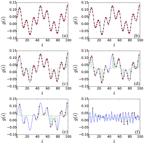
Figure 1: Comparison of the least squares $L_{2}$ (green dashed lines) and $L_{1}$ (blue solid lines) regularized regression to recover a randomly generated, discrete signal (red dots in panel (a)) obtained by randomly sampling points $i$ from the function $g(i)=\sum_{n=0}^{99}c_{n}\phi_{n}(i)$, where $\phi_{n}(i)$ is given by Eq. 8 and $i=0,\ldots,99$ is chosen so that all $n$ frequencies can be resolved. The function was constructed to be 3 sparse ($s=3$) with only $c_{0}$, $c_{4}$, and $c_{15}\neq 0$. The six panels (a)-(f) show the reconstructions for $M=1$, $0.9$, $0.8$, $0.5$, $0.2$, and $0.1$ of the input signal, respectively, included in the measurements. The red dots in panels (a)-(f) indicate the fraction of the signal that was measured and used for the reconstruction.

In Fig. 2, we measured the recovery error $d$ between the original (${\vec{g}}$) and recovered (${\vec{g}}_{rec}$) signals as a function of the fraction $M$ of the signal included and for several sparsities $s$. We define the recovery error as

$$d({\vec{g}},{\vec{g}}_{rec})=1-\frac{{\vec{g}}\cdot{\vec{g}}_{rec}}{\|{\vec{g}}\|_{2}\,\|{\vec{g}}_{rec}\|_{2}}\,,$$ (14)

where ${\vec{g}}\cdot{\vec{g}}_{rec}$ denotes the inner product between the two vectors ${\vec{g}}$ and ${\vec{g}}_{rec}$. This distance function satisfies $0\leq d\leq 2$, where $d\geq 1$ signifies a large difference between ${\vec{g}}$ and ${\vec{g}}_{rec}$ and $d=0$ indicates ${\vec{g}}={\vec{g}}_{rec}$.

For sparsity values $s=1$ and $3$, the $L_{1}$ reconstruction gives small errors ($d\sim 0$) for $M\geq 0.2$ (Fig. 2). In contrast, the error for the $L_{2}$ reconstruction method is nonzero for all $M<1$ for all $s$. For a non-sparse signal ($s=20$), the $L_{1}$ and $L_{2}$ reconstruction methods give similar errors for $M\lesssim 0.2$. In this case, the measurements truly undersample the signal, and thus providing less than $20$ measurements is not enough to constrain the $20$ nonzero coefficients $c_{j}$. However, when $M\gtrsim 0.2$, $d$ from the $L_{1}$ reconstruction method is less than that from the $L_{2}$ method and is nearly zero for $M\gtrsim 0.5$.

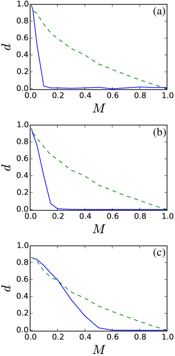
Figure 2: Comparison of the least-squares $L_{2}$ (green dashed lines) and $L_{1}$ (solid blue lines) reconstruction errors $d$ (Eq. 14) as a function of the fraction $M$ of the input signal $g(i)$ in Fig. 1 for three values of the sparsity (a) $s=1$, (b) $3$, and (c) $20$.

II.3 Sparse Basis Learning

The $L_{1}$ reconstruction method described in the previous section works well if 1) the signal has a sparse representation in some basis and 2) the basis $\Phi$ (or a subset of it) contains functions similar to the basis in which the signal is sparse. How do we proceed with signal reconstruction if we do not know a basis in which the signal is sparse? One method is to use one of the common basis sets, such as wavelets, sines, cosines, or polynomials crutchfield1987 ; judd1995 ; judd1998 . Another method is to employ sparse basis learning that identifies a basis in which a signal can be expressed sparsely. This approach is compelling because it does not require significant prior knowledge about the signal and it allows the basis to be learned even from noisy or incomplete data.

Sparse basis learning seeks to find a basis $\Phi$ that can represent an input of several signals sparsely. We identify $\Phi$ by decomposing the signal matrix ${Y=(\vec{y}_{1},\vec{y}_{2},\dots,\vec{y}_{m}})$, where $m$ is the number of signals, into the basis matrix $\Phi$ and coefficient matrix $C$,

$$Y=\Phi C\,.$$ (15)

Columns $\vec{c}_{i}$ of $C$ are the sparse coefficient vectors that represent the signals $\vec{y}_{i}$ in the basis $\Phi$. Both $C$ and $\Phi$ are unknown and can be determined by minimizing the squared differences between the signals and their representations in the basis $\Phi$ subject to the constraint that the coefficient matrix is sparse mairal2009 ; scikit-learn :

$$\hat{C},\hat{\Phi}=\min_{C,\Phi}\sum_{i=1}^{m}\left({\frac{1}{2}\|{\vec{y}}_{i}-\Phi{\vec{c}}_{i}\|_{2}^{2}+\lambda\|{\vec{c}}_{i}\|_{1}}\right)\,,$$ (16)

where $\lambda$ is a Langrange multiplier that determines the sparsity of the coefficient matrix $C$.

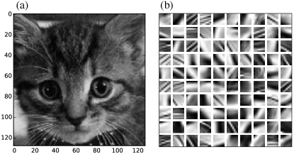
Figure 3: (a) $128\times 128$ pixel image of a cat. (b) Using the sparse learning method, we obtained $100$ $8\times 8$ pixel basis functions for the image in (a).

To illustrate the basis learning method, we show the results of sparse basis learning on the complex, two-dimensional image of a cat shown in Fig. 3 (a). To learn a sparse basis for this image, we decomposed the original image ($128\times 128$ pixels) into all possible $8\times 8$ patches, which totals $14,641$ unique patches. The patches were then reshaped into one-dimensional signals ${\vec{y}}_{i}$ each containing $64$ values. We chose $100$ basis functions (columns of $\Phi$) to sparsely represent the input matrix $Y$. Fig. 3 (b) shows the $100$ basis functions that were obtained by solving Eq. 16. The $100\times 64$ matrix $\Phi$ was reshaped into $8\times 8$ pixel basis functions before plotting. Note that some of the basis functions display complicated features, e.g., lines and ripples of different widths and angles, whereas others are more uniform.

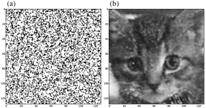
Figure 4: (a) A random collection of pixels (sampling mask) that represents $30\%$ of the image in Fig. 3 (a). (b) Sparse basis learning reconstruction of the image using samples of the image at the locations of the black pixels in (a).

To demonstrate the utility of the sparse basis learning method, we seek to recover the image in Fig. 3 (a) from an undersampled version using the learned basis functions in Fig. 3 (b) and then performing sparse reconstruction (Eq. 6) for each $8\times 8$ patch of the undersampled image. For this example, we randomly sampled $\approx 30$% of the original image. In Fig. 4 (a), the black pixels indicate the random pixels used for the sparse reconstruction of the undersampled image. We decompose the undersampled image into all possible $8\times 8$ patches, using only the measurements marked by the black pixels in the sampling mask in Fig. 4 (a). While the reconstruction of the image in Fig. 4 (b) is somewhat grainy, this reconstruction method clearly resembles the original image even when it is $70$% undersampled.

In this work, we show that one may also use incomplete data to learn a sparse basis. For example, the case of a discrete representation of a two-dimensional system of ODEs is the same problem as basis learning for image reconstruction (Fig. 3). However, learning the basis from solutions of the system of ODEs, does not provide full sampling of the signal (i.e. the right-hand side of the system of ODEs in Eq. 1), because the dynamics of the system is strongly affected by the fixed point structure and the functions are not uniformly sampled.

To learn a basis from incomplete data, we decompose the signal into patches of a given size and then fill in the missing values with random numbers. We convert the padded patches (i.e. original plus random signal) into a signal matrix $Y$ and learn a basis $\Phi$ to sparsely represent the signal by solving Eq. 16. To recover the signal, we find a sparse representation ${\hat{c}}$ of the unpadded signal (i.e. without added random values) in the learned basis $\Phi$ by solving Eq. 12, where $P$ is the matrix that selects only the signal entries that have been measured. When then obtain the reconstructed patch by taking the product $\Phi{\hat{c}}$. We repeat this process for each patch to reconstruct the full domain. For cases in which we obtain different values for the signal at the same location from different patches, we average the result.

II.4 Models

We test our methods for the reconstruction of systems of ODEs using synthetic data, i.e. data generated by numerically solving systems of ODEs, which allows us to test quantitatively the accuracy as a function of the amount of data used in the reconstruction. We present results from systems of ODEs in one, two, and three dimensions with increasing complexity in the dynamics. For an ODE in one dimension (1D), we only need to reconstruct one nonlinear function $f_{1}$ of one variable $x_{1}$. In two dimensions (2D), we need to reconstruct two functions ($f_{1}$ and $f_{2}$) of two variables ($x_{1}$ and $x_{2}$), and in three dimensions (3D), we need to reconstruct three functions ($f_{1}$, $f_{2}$, and $f_{3}$) of three variables ($x_{1}$, $x_{2}$, and $x_{3}$) to reproduce the dynamics of the system. Each of the systems that we study possesses a different fixed point structure in phase space. The 1D model has two stable fixed points and one unstable fixed point, and thus all trajectories evolve toward one of the stable fixed points. The 2D model has one saddle point and one oscillatory fixed point with closed orbits as solutions. The 3D model we study has no stable fixed points and instead possesses chaotic dynamics on a strange attractor.

1D model

For 1D, we study the Reynolds model for the immune response to infection day1 :

$$\frac{dx_{1}}{dt}=f_{1}(x_{1})=k_{pg}x_{1}\left(1-\frac{x_{1}}{x_{\infty}}\right)-\frac{k_{pm}s_{m}x_{1}}{\mu_{m}+k_{mp}x_{1}}\,,$$ (17)

where the pathogen load $x_{1}$ is unitless, and the other parameters $k_{pg}$, $k_{pm}$, $k_{mp}$, and $s_{m}$ have units of inverse hours. The right-hand side of Eq. 17 is the sum of two terms. The first term enables logistic growth of the pathogen load. In the absence of any other terms, any positive initial value will cause $x_{1}$ to grow logistically to the steady-state value $x_{\infty}$. The second term mimics a local, non-specific response to an infection, which reduces the pathogen load. For small values of $x_{1}$, the decrease is proportional to $x_{1}$. For larger values of $x_{1}$, the decrease caused by the second term is constant.

We employed the parameter values $k_{pg}=0.6$, $x_{\infty}=20$, $k_{pm}=0.6$, $s_{m}=0.005$, $\mu_{m}=0.002$, and $k_{mp}=0.01$, which were used in previous studies of this ODE model day1 ; mai2015 . In this parameter regime, Eq. 17 exhibits two stable fixed points at $x_{1}=0$ and $19.49$ and one unstable fixed point, separating the two stable fixed points, at $x_{1}=0.31$ (Fig. 5). As shown in Fig. 6, solutions to Eq. 17 with initial conditions $0\leq x_{1}\leq 0.31$ are attracted to the stable fixed point at $x_{1}=0$, while solutions with initial conditions $x_{1}>0.31$ are attracted to the stable fixed point at $x_{1}=19.49$.

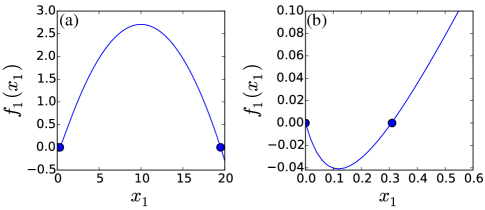
Figure 5: (a) The function $f_{1}(x_{1})$ for the Reynolds ODE model in one spatial dimension (Eq. 17) for the pathogen load in the range $0\leq x_{1}\leq 20$. Fixed points are marked by solid circles. (b) Close up of $f_{1}(x_{1})$ near the stable fixed point at $x_{1}=0$ and unstable fixed point at $x_{1}=0.31$. These two fixed points are difficult to discern on the scale shown in panel (a). Trajectories with initial conditions between $x_{1}=0$ and $0.31$ will move towards the stable fixed point at $x_{1}=0$, while initial conditions with $x_{1}>0.31$ will move toward the fixed point at $x_{1}=19.49$.

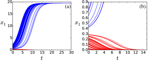
Figure 6: (a) Pathogen load $x_{1}$ as a function of time $t$ in the range $0\leq t\leq 30$ for the Reynolds ODE model in one spatial dimension (Eq. 17). (b) Close up of the region $0\leq t\leq 15$, which highlights the behavior of the system near the unstable fixed point at $x_{1}=0.31$. Solutions (red solid lines) with initial conditions $0\leq x_{1}\leq 0.31$ are attracted to the stable fixed point at $x_{1}=0$, while solutions (blue solid lines) with initial conditions $x_{1}>0.31$ are attracted to the stable fixed point at $x_{1}=19.49$.

2D model

In 2D, we focused on the Lotka-Volterra system of ODEs that describe predator-prey dynamics murray2002 :

$$\frac{dx_{1}}{dt} =f_{1}(x_{1},x_{2})=\alpha\,x_{1}-\beta\,x_{1}x_{2}$$ (18)

$$\frac{dx_{2}}{dt} =f_{2}(x_{1},x_{2})=-\gamma\,x_{2}+\delta\,x_{1}x_{2}\,,$$

where $x_{1}$ and $x_{2}$ describe the prey and predator population sizes, respectively, and are unitless. In this model, prey have a natural growth rate $\alpha$. In the absence of predators, the prey population $x_{1}$ would grow exponentially with time. With predators present, the prey population decreases at a rate proportional to the product of both the predator and prey populations with a proportionality constant $\beta$ (with units of inverse time). Without predation, the predator population $x_{2}$ would decrease at death rate $\gamma$. With the presence of prey $x_{1}$, the predator population grows proportional to the product of the two population sizes $x_{1}$ and $x_{2}$ with a proportionality constant $\delta$ (with units of inverse time).

For the Lotka-Volterra system of ODEs, there are two fixed points, one at $x_{1}=0$ and $x_{2}=0$ and one at $x_{1}=\gamma/\delta$ and $x_{2}=\alpha/\beta$. The stability of the fixed points is determined by the eigenvalues of the Jacobian matrix evaluated at the fixed points. The Jacobian of the Lotka-Volterra system is given by

$$J_{LV}=\begin{pmatrix}\alpha-\beta x_{2}&-\beta x_{1}\\ \delta x_{2}&-\gamma+\delta x_{1}\end{pmatrix}\,.$$ (19)

The eigenvalues of the Jacobian $J_{LV}$ at the origin are ${\cal J}_{1}=\alpha$, ${\cal J}_{2}=-\gamma$. Since the model is restricted to positive parameters, the fixed point at the origin is a saddle point. The interpretation is that for small populations of predator and prey, the predator population decreases exponentially due to the lack of a food source. While unharmed by the predator, the prey population can grow exponentially, which drives the system away from the zero population state, $x_{1}=0$ and $x_{2}=0$.

The eigenvalues of the Jacobian $J_{LV}$ at the second fixed point $x_{1}=\gamma/\delta$ and $x_{2}=\alpha/\beta$ are purely imaginary complex conjugates, ${\cal J}_{1}=-i\sqrt{\alpha\gamma}$ and ${\cal J}_{2}=i\sqrt{\alpha\gamma}$, where $i^{2}=-1$. The purely imaginary fixed point causes trajectories to revolve around it and form closed orbits. The interpretation of this fixed point is that the predators decrease the number of prey, then the predators begin to die due to a lack of food, which in turn allows the prey population to grow. The growing prey population provides an abundant food supply for the predator, which allows the predator to grow faster than the food supply can sustain. The prey population then decreases and the cycle repeats. For the results below, we chose the parameters $\alpha=0.4$, $\beta=0.4$, $\gamma=0.1$, and $\delta=0.2$ for the Lotka-Volterra system, which locates the oscillatory fixed point at $x_{1}=0.5$ and $x_{2}=1.0$ (Fig. 7).

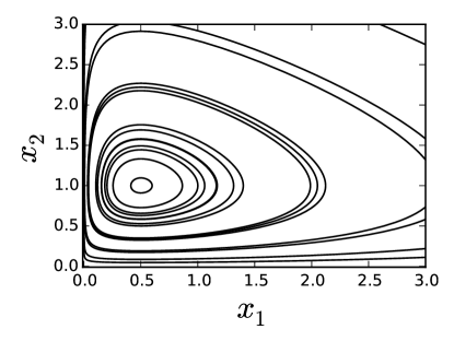
Figure 7: Solutions of the two-dimensional Lotka-Volterra ODE model (Eq. 18) with $\alpha=0.4$, $\beta=0.4$, $\gamma=0.1$, and $\delta=0.2$ plotted parametrically ($x_{2}(t)$ versus $x_{1}(t)$) for $15$ random initial conditions in the domain $0\leq x_{1}\leq 0.5$ and $0\leq x_{2}\leq 1$. This model has an unstable fixed point at $x_{1}=0$ and $x_{2}=0$ and an oscillatory fixed point at $x_{1}=0.5$ and $x_{2}=1$.

3D model

In 3D, we focused on the Lorenz system of ODEs lorenz1963 , which describes fluid motion in a container that is heated from below and cooled from above:

$$\frac{dx_{1}}{dt} =f_{1}(x_{1},x_{2},x_{3})=\sigma(x_{2}-x_{1})$$ (20)

$$\frac{dx_{2}}{dt} =f_{2}(x_{1},x_{2},x_{3})=x_{1}(\rho-x_{3})-x_{2}$$

$$\frac{dx_{3}}{dt} =f_{3}(x_{1},x_{2},x_{3})=x_{1}x_{2}-\beta x_{3}\,,$$

where $\sigma,\rho,\beta$ are positive, dimensionless parameters that represent properties of the fluid. In different parameter regimes, the fluid can display quiescent, convective, and chaotic dynamics. The three dimensionless variables $x_{1}$, $x_{2}$, and $x_{3}$ describe the intensity of the convective flow, temperature difference between the ascending and descending fluid, and spatial dependence of the temperature profile, respectively.

The system possesses three fixed points at $(x_{1},x_{2},x_{3})=(0,0,0)$, $(-\beta^{1/2}(\rho-1)^{1/2},-\beta^{1/2}(\rho-1)^{1/2},\rho-1)$, and $(\beta^{1/2}(\rho-1)^{1/2},\beta^{1/2}(\rho-1)^{1/2},\rho-1)$. The Jacobian of the system is given by

$$J_{L}=\begin{pmatrix}-\sigma&\sigma&0\\ \rho-x_{3}&-1&-x_{1}\\ x_{2}&x_{1}&-\beta\end{pmatrix}\,.$$ (21)

When we evaluate the Jacobian (Eq. 21) at the fixed points, we find that each of the three eigenvalues possesses two stable and one unstable eigendirection in the parameter regime $\sigma=10$, $\rho=28$ and $\beta=8/3$. With these parameters, the Lorenz system displays chaotic dynamics with Lyapunov exponents $\ell_{1}=0.91$, $\ell_{2}=0.0$, and $\ell_{3}=-14.57$. In Fig. 8, we show the time evolution of two initial conditions in $x_{1}$-$x_{2}$-$x_{3}$ configuration space for this parameter regime.

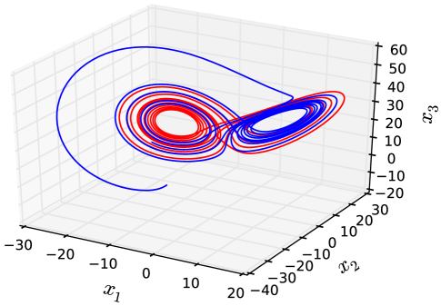
Figure 8: Solutions of the three-dimensional Lorenz ODE model (Eq. 20) with $\sigma=10$, $\rho=28$, and $\beta=8/3$ plotted parametrically in the $x_{1}$-$x_{2}$-$x_{3}$ plane for two initial conditions $(x_{1},x_{2},x_{3})=(-7.57,11.36,9.51)$ (red solid line) and $(-12.17,-5.23,-11.60)$ (blue solid line). For this parameter regime, the system has three unstable fixed points, lives on the Lorenz attractor, and possesses chaotic dynamics.

III Results

In this section, we present the results of our methodology for ODE reconstruction of data generated from the three systems of ODEs described in Sec. II.4. For each system, we measure the accuracy of the reconstruction as a function of the size of the sections used to decompose the signal for basis learning, the sampling time interval between time series measurements, and the number of trajectories. For each model, we make sure that the total integration time is sufficiently large that the system can reach the stable fixed points or sample the chaotic attractor in the case of the Lorenz system.

III.1 Reconstruction of ODEs in 1D

We first focus on the reconstruction of the Reynolds ODE model in 1D (Eq. 17) using time series data. We discretized the domain $0\leq x_{1}\leq 19.5$ using $256$ points, $i=0,\ldots,255$. Because the unstable fixed point at $x_{1}=0.31$ is much closer to the stable fixed point at $x_{1}=0$ than to the stable fixed point at $x_{1}=19.49$, we sampled more frequently in the region $0\leq x_{1}\leq 0.6$ compared to the region $0.6<x_{1}\leq 19.5$. In particular, we uniformly sampled $128$ points from the small domain, and uniformly sampled the same number of points from the large domain.

In Fig. 9, we show the error $d$ (Eq. 14) in recovering the right-hand side of Eq. 17 ($f_{1}(x_{1})$) as a function of the size $p$ of the patches used for basis learning. Each data point in Fig. 9 represents an average over $20$ reconstructions using $N_{t}=10$ trajectories with a sampling time interval $\Delta t=1$. We find that the error $d$ achieves a minimum below $10^{-3}$ in the patch size range $30<p<50$. Basis sizes that are too small do not adequately sample $f_{1}(x_{1})$, while basis patches that are too large do not include enough variability to select a sufficiently diverse basis set to reconstruct $f_{1}(x_{1})$. For example, in the extreme case that the basis patch size is the same size as the signal, we are only able to learn the input data itself, which may be missing data. For the remaining studies of the 1D model, we set $p=50$ as the basis patch size.

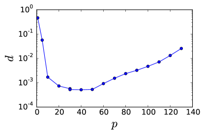
Figure 9: Error $d$ in the ODE reconstruction for the 1D Reynolds model (Eq. 17) as a function of the patch size $p$ used for basis learning using $N_{t}=10$ trajectories with sampling time interval $\Delta t=1$.

In Fig. 10, we plot the error in the reconstruction of $f_{1}(x_{1})$ as a function of the sampling time interval $\Delta t$ for several numbers of trajectories $N_{t}=1$, $2$, $20$, $50$, and $200$. We find that the error decreases with the number of trajectories used in the reconstruction. For $N_{t}=1$, the error is large with $d>0.1$. For large numbers of trajectories (e.g. $N_{t}=200$), the error decreases with decreasing $\Delta t$, reaching $d\sim 10^{-5}$ for small $\Delta t$. The fact that the error in the ODE reconstruction increases with $\Delta t$ is consistent with notion that the accuracy of the numerical derivative of each trajectory decreases with increasing sampling interval. In Fig. 11, we show the error in the reconstruction of $f_{1}(x_{1})$ as a function of the total integration time $t_{end}$. We find that $d$ decreases strongly as $t_{end}$ increases for $t_{end}<20$. For $t_{end}>20$, $d$ reaches a plateau value below $10^{-4}$, which depends weakly on $\Delta t$. For characteristic time scales $t>20$, the Reynolds ODE model reaches one of the two stable fixed points, and therefore $d$ becomes independent of $t_{end}$.

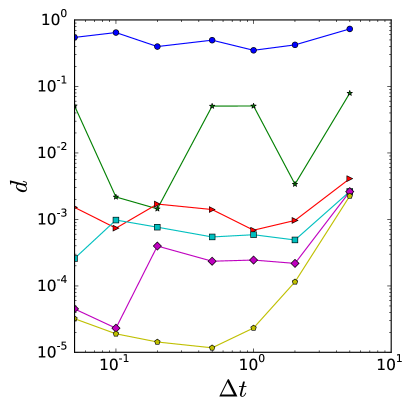
Figure 10: Reconstruction error $d$ for the 1D Reynolds model as a function of the sampling interval $\Delta t$ for several different numbers of trajectories $N_{t}=1$ (circles), $5$ (stars), $10$ (triangles), $20$ (squares), $50$ (diamonds), and $200$ (pentagons) used in the reconstruction. The data for each $N_{t}$ is averaged over $20$ independent reconstructions.

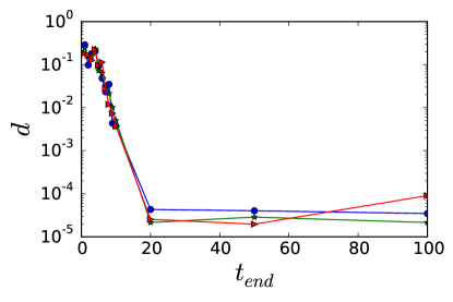
Figure 11: Reconstruction error $d$ for the 1D Reynolds ODE model as a function of the total integration time $t_{end}$ used for the reconstruction for $N_{t}=20$ trajectories at several values of the sampling time $\Delta t=0.05$ (circles), $0.1$ (stars), and $0.5$ (triangles).

In Fig. 12, we compare accurate (using $N_{t}=50$ and $\Delta t=0.1$) and inaccurate (using $N_{t}=10$ and $\Delta t=5$) reconstructions of $f_{1}(i_{1})$ for the 1D Reynolds ODE model. Note that we plot $f_{1}$ as a function of the scaled variable $i_{1}$. The indexes $i_{1}=0,\ldots,127$ indicate uniformly spaced $x_{1}$ values in the interval $0\leq x_{1}\leq 0.6$, and $i_{1}=128,\ldots,256$ indicate uniformly spaced $x_{1}$ values in the interval $0.6<x_{1}\leq 19.5$.

We find that using large $\Delta t$ gives rise to inaccurate measurements of the time derivative of $x_{1}$ and, thus of $f_{1}(x_{1})$. In addition, large $\Delta t$ does not allow dense sampling of phase space, especially in regions where the trajectories evolve rapidly. The inaccurate reconstruction in Fig. 12 (b) is even worse than it seems at first glance. The reconstructed function is identically zero over a wide range of $i_{1}$ ($0\leq i_{1}\leq 50$) where $f(i_{1})$ is not well sampled, since the default output of a failed reconstruction is zero. It is a coincidence that $f_{1}(i_{1})\sim 0$ in Eq. 17 over the same range of $i_{1}$.

Figure 12: Reconstructions (solid blue lines) of $f_{1}(i_{1})$ for the 1D Reynolds ODE model in Eq. 17 using (a) $N_{t}=50$ and $\Delta t=0.1$ and (b) $N_{t}=10$ and $\Delta t=5$. $f_{1}$ is discretized using $256$ points. The indices $i_{1}=0,\ldots,127$ indicate uniformly spaced $x_{1}$ values in the interval $0\leq x_{1}\leq 0.6$, and $i_{1}=128,\ldots,256$ indicate uniformly spaced $x_{1}$ values in the interval $0.6<x_{1}\leq 19.5$. The exact expression for $f_{1}(i_{1})$ is represented by the green circles.

We now numerically solve the reconstructed 1D Reynolds ODE model for different initial conditions and times comparable to $t_{end}$ and compare these trajectories to those obtained from the original model (Eq. 17). In Fig. 13, we compare the trajectories $x_{1}(t)$ for the accurate ($d\sim 10^{-5}$; Fig. 12 (a)) and inaccurate ($d\sim 10^{-2}$; Fig. 12 (b)) representations of $f_{1}(x_{1})$ to the original model for six initial conditions. All of the trajectories for the accurate representation of $f_{1}(x_{1})$ are nearly indistinguishable from the trajectories for the original model, whereas we find large deviations between the original and reconstructed trajectories even at short times for the inaccurate representation of $f_{1}(x_{1})$.

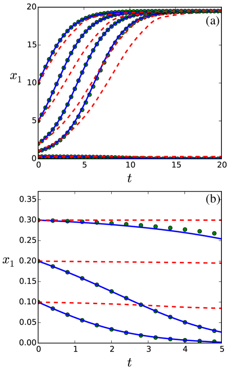
Figure 13: (a) Comparison of the trajectories $x_{1}(t)$ for the 1D Reynolds ODE model using the accurate (solid blue lines) and inaccurate (dashed red lines) reconstructions of $f_{1}(x_{1})$ shown in Fig. 12 (a) and (b), respectively, for six initial conditions: $x_{1}(0)=0.1$, $0.2$, $0.3$, $1$, $2$, $5$, and $10$. The trajectories obtained from $f_{1}(x_{1})$ in Eq. 17 are given by the open red circles. (b) Close up of the trajectories in the domain $0\leq x_{1}\leq 0.4$.

III.2 Reconstruction of Systems of ODEs in 2D

We now investigate the reconstruction accuracy of our method for the Lotka-Volterra system of ODEs in 2D. We find that the results are qualitatively similar to those for the 1D Reynolds ODE model. We map the numerical derivatives for $N_{t}$ trajectories with a sampling time interval $\Delta t$ onto a $128\times 128$ grid with $0\leq x_{1},x_{2}\leq 2$. Similar to the 1D model, we find that the error in the reconstruction of $f_{1}(x_{1},x_{2})$ and $f_{2}(x_{1},x_{2})$ possesses a minimum as a function of the patch area used for basis learning, where the location and value at the minimum depends on the parameters used for the reconstruction. For example, for $N_{t}=200$, $\Delta t=0.1$, and averages over $20$ independent runs, the error reaches a minimum ($d\approx 10^{-5}$) near $p^{2}_{\rm min}\approx 100$.

In Fig. 14, we show the reconstruction error $d$ as a function of the sampling time interval $\Delta t$ for several values of $N_{t}$ from $5$ to $500$ trajectories, for a total time $t_{end}$ that allows several revolutions around the closed orbits, and for patch size $p^{2}_{\rm min}$. As in 1D, we find that increasing $N_{t}$ reduces the reconstruction error. For $N_{t}=5$, $d\sim 10^{-1}$, while $d<10^{-3}$ for $N_{t}=500$. $d$ also decreases with decreasing $\Delta t$, although $d$ reaches a plateau in the small $\Delta t$ limit, which depends on the number of trajectories included in the reconstruction.

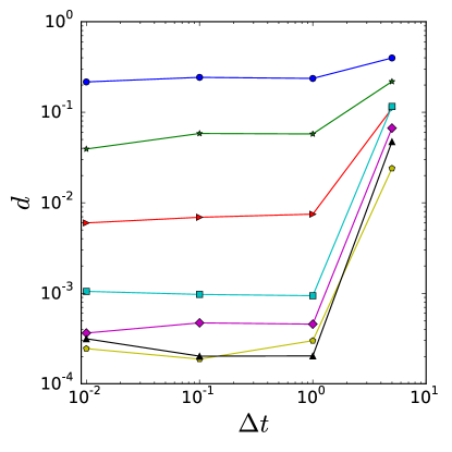
Figure 14: Reconstruction error $d$ for the 2D Lotka-Volterra model (Eq. 18) as a function of the sampling time interval $\Delta t$ for different numbers of trajectories $N_{t}=5$ (circles), $10$ (stars), $20$ (rightward triangles), $50$ (squares), $100$ (diamonds), $200$ (pentagons), and $500$ (upward triangles) averaged over $20$ independent runs.

In Figs. 15 and 16, we show examples of inaccurate ($d\sim 10^{-2}$) and accurate ($d\sim 10^{-5}$) reconstructions of $f_{1}(i_{1},i_{2})$ and $f_{2}(i_{1},i_{2})$. The indexes $i_{1,2}=0,\ldots,127$ indicate uniformly spaced $x_{1}$ and $x_{2}$ values in the interval $0\leq x_{1,2}\leq 2$. The parameters for the inaccurate reconstructions were $N_{t}=30$ trajectories and $\Delta t=5$ (enabling $f_{1}$ and $f_{2}$ to be sampled only over $2\%$ of the domain), whereas the parameters for the accurate reconstructions were $N_{t}=100$ trajectories and $\Delta t=0.01$ (enabling $f_{1}$ and $f_{2}$ to be sampled over $68\%$ of the domain). These results emphasize that even though the derivatives are undetermined over nearly one-third of the domain, we can reconstruct the functions $f_{1}$ and $f_{2}$ extremely accurately over the full domain.

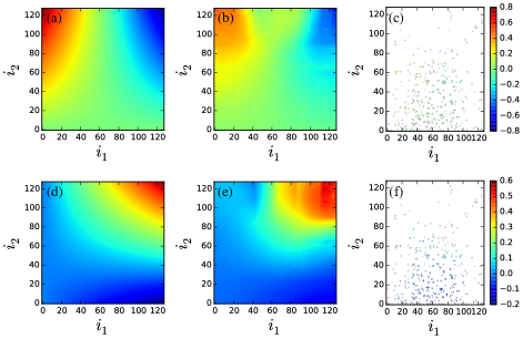
Figure 15: Example of inaccurate reconstructions of $f_{1}(i_{1},i_{2})$ and $f_{2}(i_{1},i_{2})$ (with errors $d=0.04$ and $0.03$, respectively) for the 2D Lotka-Volterra system of ODEs (18). The indexes $i_{1,2}=0,\ldots,127$ indicate uniformly spaced $x_{1}$ and $x_{2}$ values in the interval $0\leq x_{1,2}\leq 2$. Panels (a) and (d) give the exact functions $f_{1}(i_{1},i_{2})$ and $f_{2}(i_{1},i_{2})$, panels (b) and (e) give the reconstructions, and panels (c) and (f) indicate the $i_{1}$-$i_{2}$ values that were sampled (2% of the $128\times 128$ grid). The white regions in panel (c) and (f) indicate missing data. In the top row, the color scale varies from $-0.8$ to $0.8$ (from dark blue to red). In the bottom row, the color scale varies from $-0.2$ to $0.6$ (from dark blue to red). This reconstruction was obtained using $N_{t}=30$ trajectories, a sampling interval $\Delta t=5$, and a basis patch area $p^{2}=625$.

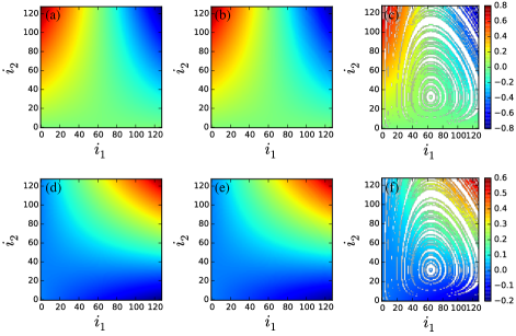
Figure 16: Example of accurate reconstructions of $f_{1}(i_{1},i_{2})$ and $f_{2}(i_{1},i_{2})$ (with errors $d=4\times 10^{-5}$ and $5\times 10^{-5}$, respectively) for the 2D Lotka-Volterra system of ODEs (18). The indexes $i_{1,2}=0,\ldots,128$ indicate uniformly spaced $x_{1}$ and $x_{2}$ values in the interval $0\leq x_{1,2}\leq 2$. Panels (a) and (d) give the exact functions $f_{1}(i_{1},i_{2})$ and $f_{2}(i_{1},i_{2})$, panels (b) and (e) give the reconstructions, and panels (c) and (f) indicate the $i_{1}$-$i_{2}$ values that were sampled ($68\%$ of the $128\times 128$ grid). The white regions in panel (c) and (f) indicate missing data. The color scales are the same as in Fig. 15. This reconstruction was obtained using $N_{t}=100$ trajectories, a sampling interval of $\Delta t=0.01$, and a basis patch area $p^{2}=625$.

Using the reconstructions of $f_{1}$ and $f_{2}$, we solved for the trajectories $x_{1}(t)$ and $x_{2}(t)$ (for times comparable to $t_{end}$) and compared them to the trajectories from the original Lotka-Volterra model (Eq. 18). In Fig. 17 (a) and (b), we show parametric plots ($x_{2}(t)$ versus $x_{1}(t)$) for the inaccurate (Fig. 15) and accurate (Fig. 16) reconstructions of $f_{1}$ and $f_{2}$, respectively. We solved both the inaccurate and accurate models with the same four sets of initial conditions. For the inaccurate reconstruction, most of the trajectories from the reconstructed ODE system do not match the original trajectories. In fact, some of the trajectories spiral outward and do not form closed orbits. In contrast, for the accurate reconstruction, the reconstructed trajectories are very close to those of the original model and all possess closed orbits.

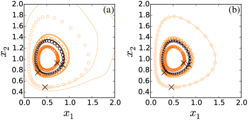
Figure 17: Parametric plots of the trajectories $x_{1}(t)$ and $x_{2}(t)$ (solid lines) for the (a) inaccurate and (b) accurate reconstructions of $f_{1}$ and $f_{2}$ in Figs. 15 and 16, respectively, for four different initial conditions indicated by the crosses. The open circles indicate the trajectories from the Lotka-Volterra system of ODEs (Eq. 18).

III.3 Reconstruction of systems of ODEs in 3D

For the Lorenz ODE model, we need to reconstruct three functions of three variables: $f_{1}(x_{1},x_{2},x_{3})$, $f_{2}(x_{1},x_{2},x_{3})$, and $f_{3}(x_{1},x_{2},x_{3})$. Based on the selected parameters $\sigma=10$, $\rho=28$ and $\beta=8/3$, we chose a $32\times 32\times 32$ discretization of the domain $-21\leq x_{1}\leq 21$, $-29\leq x_{2}\leq 29$, and $-2\leq x_{3}\leq 50$. We employed patches of size $10\times 10$ from each of the $32$ slices (along $x_{3}$) of size $32\times 32$ (in the $x_{1}$-$x_{2}$ plane) to perform the basis learning.

In Fig. 18, we plot the reconstruction error $d$ versus the sampling time interval $\Delta t$ for several $N_{t}$ from $500$ to $10^{4}$ trajectories. As found for the 1D and 2D ODE models, the reconstruction error decreases with decreasing $\Delta t$ and increasing $N_{t}$. $d$ reaches a low-$\Delta t$ plateau that depends on the value of $N_{t}$. For $N_{t}=10^{4}$, the low-$\Delta t$ plateau value for the reconstruction error approaches $d\sim 10^{-3}$.

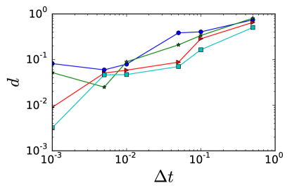
Figure 18: Reconstruction error $d$ plotted versus the sampling time interval $\Delta t$ for the 3D Lorenz model Eq. (20) for several different numbers of trajectories $N_{t}=500$ (circles), $1000$ (stars) $5000$ (rightward triangles), and $10000$ (squares). Each data point is averaged over $20$ independent reconstructions.

In Fig. 19, we visualize the reconstructed functions $f_{1}$, $f_{2}$, and $f_{3}$ for the Lorenz system of ODEs. Panels (a)-(c) represent $f_{1}$, (d)-(f) represent $f_{2}$, and (g)-(i) represent $f_{3}$. The 3D domain is broken into $32$ slices (along $x_{3}$) of $32\times 32$ grid points in the $x_{2}$-$x_{3}$ plane. Panels (a), (d), and (g) give the original functions $f_{1}$, $f_{2}$, and $f_{3}$ in the Lorenz system of ODEs (Eq. 20). Panels (b), (e), and (h) give the reconstructed versions of $f_{1}$, $f_{2}$, and $f_{3}$, and panels (c), (f), and (i) provide the data that was used for the reconstructions (with white regions indicating missing data). The central regions of the functions are recovered with high accuracy. (The edges of the domain were not well-sampled, and thus the reconstruction was not as accurate.) These results show that even for chaotic systems in 3D we are able to achieve accurate ODE reconstruction. In Fig. 20, we compare trajectories from the reconstructed functions to those from the original Lorenz system of ODEs for times comparable to the inverse of the largest Lyapunov exponent. In this case, we find that some of the the trajectories from the reconstructed model closely match those from the original model, while others differ from the trajectories of the original model. Since chaotic systems are extremely sensitive to initial conditions, we expect that all trajectories of the reconstructed model will differ from the trajectories of the original model at long times. Despite this, the trajectories from the reconstructed model display chaotic dynamics with similar Lyapunov exponents to those for the Lorenz system of ODEs, and thus we are able to recover the controlling dynamics of the original model.

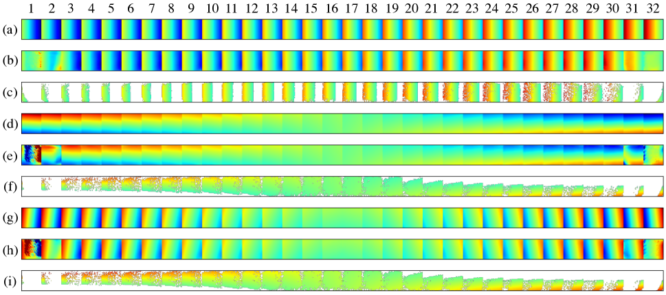
Figure 19: Reconstruction of the Lorenz system of ODEs in 3D (Eq. 20) using the sampling time interval $\Delta t=10^{-2}$ and $N_{t}=10^{4}$ trajectories. Panels (a)-(c) indicate $f_{1}(i_{1})$, (d)-(f) indicate $f_{2}(i_{2})$, and (g)-(i) indicate $f_{3}(i_{3})$, where the indexes $i_{1}$, $i_{2}$, and $i_{3}$ represent uniformly spaced $x_{1}$, $x_{2}$, and $x_{3}$ values on the intervals $-21\leq x_{1}\leq 21$, $-29\leq x_{2}\leq 29$, and $-2\leq x_{3}\leq 50$. Each of the $32$ panels along $x_{3}$ represents a $32\times 32$ discretization of the $x_{1}$-$x_{2}$ domain. The first rows of each grouping of three (i.e. panels (a), (d), and (g)) give the original functions $f_{1}$, $f_{2}$, and $f_{3}$. The second rows of each grouping of three (i.e. panels (b), (e), and (h)) give the reconstructed versions of $f_{1}$, $f_{2}$, and $f_{3}$. The third rows of of grouping of three (i.e. panels (c), (f), and (i)) show the points in the $x_{1}$, $x_{2}$, and $x_{3}$ domain that were used for the reconstruction. The white regions indicate missing data. The color scales range from dark blue to red corresponding to the ranges of $-500\leq f_{1}(i_{1},i_{2},i_{3})\leq 500$, $-659\leq f_{2}(i_{1},i_{2},i_{3})\leq 659$, and $-742\leq f_{3}(i_{1},i_{2},i_{3})\leq 614$ for the groups of panels (a)-(c), (d)-(f), and (g)-(i), respectively.

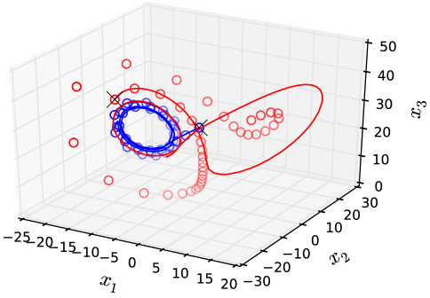
Figure 20: We compare the trajectories $x_{1}(t)$, $x_{2}(t)$, and $x_{3}(t)$ from the reconstructed (solid lines) and original (empty circles) functions $f_{1}$, $f_{2}$, and $f_{3}$ from the 3D Lorenz system of ODEs (Eq. 20) with the parameters $\sigma=10$, $\rho=28$, and $\beta=8/3$ in the chaotic regime. We plot $x_{1}$, $x_{2}$, and $x_{3}$ parametrically for two initial conditions indicated by the crosses.

IV Discussion

We developed a new method for reconstructing sets of nonlinear ODEs from time series data using machine learning methods involving sparse function reconstruction and sparse basis learning. Using only information from the system trajectories, we first learned a sparse basis, with no a priori knowledge of the underlying functions in the system of ODEs, and then reconstructed the system of ODEs in this basis. A key feature of our method is its reliance on sparse representations of the system of ODEs. Our results emphasize that sparse representations provide more accurate reconstructions of systems of ODEs than least-squares approaches.

We tested our ODE reconstruction method on time series data obtained from systems of ODEs in 1D, 2D, and 3D. In 1D, we studied the Reynolds model for the immune response to infection. In the parameter regime we considered, this system possesses only two stable fixed points, and thus all initial conditions converge to these fixed points in the long-time limit. In 2D, we studied the Lotka-Volterra model for predator-prey dynamics. In the parameter regime we studied, this system possesses an oscillatory fixed point with closed orbits. In 3D, we studied the Lorenz model for convective flows. In the parameter regime we considered, the system displays chaotic dynamics on a strange attractor.

For each model, we measured the error in the reconstructed system of ODEs as a function of parameters of the reconstruction method including the sampling time interval $\Delta t$, number of trajectories $N_{t}$, total time $t_{end}$ of the trajectory, and size of the patches used for basis function learning. In general, the error decreases as more data is used for the reconstruction. We determined the parameter regimes for which we could achieve highly accurate reconstruction with errors $d<10^{-3}$. We then generated trajectories from the reconstructed systems of ODEs and compared them to the trajectories of the original models. For the 1D model with two stable fixed points, we were able to achieve extremely accurate reconstruction and recapitulation of the trajectories of the original model. Our reconstruction for the 2D model is also accurate and is able to achieve closed orbits for most initial conditions. For some of the initial conditions, smaller sampling time intervals and longer trajectories were needed to achieve reconstructed solutions with closed orbits. In future studies, we will investigate methods to add a constraint that imposes the constant of the motion on the reconstruction method, which will allow us to use larger sampling time intervals and shorter trajectories and still achieve closed orbits. For the 3D chaotic Lorenz system, we can only match the trajectories of the reconstructed and original systems for times that are small compared to the inverse of the largest Lyapunov exponent. Even though the trajectories of the reconstructed and original systems will diverge, we have shown that the reconstructed and original systems of ODEs possess dynamics with similar Lyapunov exponents. Now that we have validated this ODE reconstruction method on known deterministic systems of ODEs and determined the parameter regimes that yield accurate reconstructions, we will employ this method in future studies to identify new systems of ODEs using time series data from experimental systems for which there is no currently known system of ODEs.

- (1) E. N. Lorenz, “Deterministic nonperiodic flow,” Journal of the Atmospheric Sciences 20 (1963) 130.
- (2) C. O. Weiss and J. Brock, “Evidence for Lorenz-type chaos in a laser,” Physical Review Letters 57 (1986) 2804.
- (3) K. M. Cuomo, A. V. Oppenheim, and S. H. Strogatz, “Synchronization of Lorenz-based chaotic circuits with applications to communications,” IEEE Transactions on Circuits and Systems II: Analog and Digital Signal Processing 40 (1993) 626.
- (4) H. Aref, “The development of chaotic advection,” Physics of Fluids 14 (2002) 1315.
- (5) M. E. Csete and J. C. Doyle, “Reverse engineering of biological complexity,” Science 295 (2002) 1664.
- (6) A. F. Villaverde and J. R. Banga, “Reverse engineering and identification in systems biology: Strategies, perspectives and challenges,” Journal of the Royal Society Interface 11 (2014) 2013.0505.
- (7) A. S. Perelson and P. W. Nelson, “Mathematical analysis of HIV- dynamics in vivo,” SIAM Rev. 41 (1999) 3.
- (8) D. S. Callaway and A. S. Perelson, “HIV- infection and low steady state viral loads,” B. Math. Biol. 64 (2002) 29.
- (9) P. W. Nelson and A. S. Perelson, “Mathematical analysis of delay differential equation models of HIV- infection,” Math Biosci. 179 (2002) 73.
- (10) H. Dahari, E. Shudo, R. M. Ribeiro, and A. S. Perelson, “Modeling complex decay profiles of hepatitis B virus during antiviral therapy,” Hepatology 49 (2009) 32.
- (11) S. A. Gourley, Y. Kuang, and J. D. Nagy, “Dynamics of a delay differential equation model of hepatitis B virus infection,” Journal of Biological Dynamics 2 (2008) 140.
- (12) B. Hancioglu, D. Swigon, and G. Clermont, “A dynamical model of human immune response to influenza A virus infection,” Journal of Theoretical Biology 246 (2007) 70.
- (13) A. S. Perelson, “Modeling viral and immune system dynamics,” Nat. Rev. Immunol. 2 (2002) 28.
- (14) A. Reynolds, J. Rubin, G. Clermont, J. Day, Y. Vodovotz, and G. B. Ermentrout, “A reduced mathematical model of the acute inflammatory response: I. Derivation of model and analysis of anti-inflammation.” Journal of Theoretical Biology 242 (2006) 220.
- (15) J. Day, J. Rubin, Y. Vodovotz, C. C. Chow, A. Reynolds, and G. Clermont, “A reduced mathematical model of the acute inflammatory response II. Capturing scenarios of repeated endotoxin administration.” Journal of Theoretical Biology 242 (2006) 237.
- (16) R. Arditi and L. R. Ginzburg, “Coupling in predator-prey dynamics: Ratio-dependence,” Journal of Theoretical Biology 139 (1989) 311.
- (17) E. Baake, M. Baake, H. G. Bock, and K. M. Briggs, “Fitting ordinary differential equations to chaotic data,” Physical Review A 45 (1992) 5524.
- (18) S. Marino and E. O. Voit, “An automated procedure for the extraction of metabolic network information from time series data,” Journal of Bioinformatics and Computational Biology 4 (2006) 665.
- (19) J. Bongard and H. Lipson, “Automated reverse engineering of nonlinear dynamical systems,” Proc. Nat. Acad. Sci. 104 (2007) 9943.
- (20) M. D. Schmidt and H. Lipson, “Data-mining dynamical systems: Automated symbolic system identification for exploratory analysis,” (ASME 2008 9th Biennial Conference on Engineering Systems Design and Analysis. American Society of Mechanical Engineers, 2008).
- (21) M. D. Schmidt and H. Lipson, “Distilling free-form natural laws from experimental data,” Science 324 (2009) 81.
- (22) B. A. Olshausen and D. J. Field, “Sparse coding with an overcomplete basis set: A strategy employed by V1?,” Vision Research 37 (1997) 3311.
- (23) M. Aharon, M. Elad, and A. Bruckstein, “K-SVD: An Algorithm for designing overcomplete dictionaries for sparse representation,” IEEE Transactions on Signal Processing 54 (2006) 4311.
- (24) M. Aharon and M. Elad, “Sparse and redundant modeling of image content using an image-signature-dictionary,” SIAM Journal on Imaging Sciences 1 (2008) 228.
- (25) E. C. Smith and M. S. Lewicki, “Efficient auditory coding,” Nature 439 (2006) 978.
- (26) R. Raina, A. Battle, H. Lee, B. Packer, and A. Y. Ng, “Self-taught learning: Transfer learning from unlabeled data,” Proceedings of the 24th International Conference on Machine Learning (ACM) (2007) 759.
- (27) J. Mairal, J. Ponce, G. Sapiro, A. Zisserman, and F. R. Bach, “Supervised dictionary learning,” Advances in Neural Information Processing Systems 21 (2009) 1033.
- (28) E. J. Candès, J. Romberg, and T. Tao, “Robust uncertainty principles: Exact signal reconstruction from highly incomplete frequency information,” IEEE Transactions on Information Theory 52 (2006) 489.
- (29) D. L. Donoho, M. Elad, and V. N. Temlyakov, “Stable recovery of sparse overcomplete representations in the presence of noise,” IEEE Transactions on Information Theory 52 (2006) 6.
- (30) E. J. Candès “Compressive sampling,” Proceedings of the International Congress of Mathematicians 3 (2006) 1433.
- (31) D. L. Donoho, “Compressed sensing,” IEEE Transactions on Information Theory 52 (2006) 1289.
- (32) E. J. Candès and J. Romberg, “Quantitative robust uncertainty principles and optimally sparse decompositions,” Foundations of Computational Mathematics 6 (2006) 227.
- (33) E. J. Candès, J. Romberg, and T. Tao. “Stable signal recovery from incomplete and inaccurate measurements,” Communications on Pure and Applied Mathematics 59 (2006) 1207.
- (34) R. G. Baraniuk, “Compressive sensing,” IEEE Signal Processing Magazine 24 (2007) 118.
- (35) E. J. Candès and M. B. Wakin, “An introduction to compressive sampling,” IEEE Signal Processing Magazine 25 (2008) 21.
- (36) D. L. Donoho and J. Tanner, “Precise undersampling theorems,” Proceedings of the IEEE 98 (2010) 913.
- (37) M. Lustig, D. L. Donoho, and J. M. Pauly, “Sparse MRI: The application of compressed sensing for rapid MR imaging,” Magnetic Resonance in Medicine 58 (2007) 1182.
- (38) M. Lustig, D.L. Donoho, J.M. Santos, and J.M. Pauly, “Compressed sensing MRI,” IEEE Signal Processing Magazine 25 (2008) 72.
- (39) J. P. Haldar, D. Hernando, and Z.-P. Liang, “Compressed-sensing MRI with random encoding,” IEEE Transactions on Medical Imaging 30 (2011) 893.
- (40) M. Duarte, M. Davenport, D. Takhar, J. Laska, T. Sun, K. Kelly, and R. G. Baraniuk, “Single-pixel imaging via compressive sampling, IEEE Signal Processing Mag. 25 (2008) 83.
- (41) J. Yang, J. Wright, T. S. Huang, and Y. Ma, “Image super-resolution via sparse representation,” IEEE Transactions on Image Processing 19 (2010) 2861.
- (42) D. L. Donoho, “For most large underdetermined systems of linear equations the minimal norm solution is also the sparsest solution,” Communications on Pure and Applied Mathematics 59 (2006) 797.
- (43) F. Pedregosa, G. Varoquaux, A. Gramfort, V. Michel, B. Thirion, O. Grisel, M. Blondel, P. Prettenhofer, R. Weiss, V. Dubourg, and J. Vanderplas, “Scikit-learn: Machine learning in Python,” Journal of Machine Learning Research 12 (2011) 2825.
- (44) J. P. Crutchfield and B. S. McNamara, “Equations of motion from a data series,” Complex Systems 1 (1987) 417.
- (45) K. Judd and A. Mees, “On selecting models for nonlinear time series,” Physica D: Nonlinear Phenomena 82 (1995) 426.
- (46) K. Judd and A. Mees, “Embedding as a modeling problem,” Physica D: Nonlinear Phenomena 120 (1998) 273.
- (47) J. Mairal, F. Bach, J. Ponce, and G. Sapiro, “Online dictionary learning for sparse coding,” Proceedings of the 26th Annual International Conference on Machine Learning (2009) 689.
- (48) M. Mai, K. Wang, G. Huber, M. Kirby, M. D. Shattuck, and C. S. O’Hern, “Outcome prediction in mathematical models of immune response to infection,” PloS One 10 (2015) e0135861.
- (49) J. D. Murray, “Mathematical Biology I: An Introduction,” Interdisciplinary Applied Mathematics 17 (2002).