Linear redshift space distortions for cosmic voids based on galaxies in redshift space

Abstract

Cosmic voids found in galaxy surveys are defined based on the galaxy distribution in redshift space. We show that the large scale distribution of voids in redshift space traces the fluctuations in the dark matter density field $\hat{\delta}(\mbox{\boldmath$k$})$ (in Fourier space with $\mu$ being the line of sight projected $k$-vector): $\hat{\delta}_{\rm v}^{s}(\mbox{\boldmath$k$})=(1+\beta_{\rm v}\mu^{2})\,b^{s}_{\rm v}\,\hat{\delta}(\mbox{\boldmath$k$})$, with a beta factor that will be in general different than the one describing the distribution of galaxies. Only in case voids could be assumed to be quasi-local transformations of the linear (Gaussian) galaxy redshift space field, one gets equal beta factors $\beta_{\rm v}=\beta_{\rm g}=f/b_{\rm g}$ with $f$ being the growth rate, and $b_{\rm g}$, $b^{s}_{\rm v}$ being the galaxy and void bias on large scales defined in redshift space. Indeed, in our mock void catalogs we measure void beta factors being in good agreement with the galaxy one. Further work needs to be done to confirm the level of accuracy of the beta factor equality between voids and galaxies, but in general the void beta factor needs to be considered as a free parameter for linear RSD studies.

I Introduction

Cosmic voids have drawn attention in the last few years due to their potential power to constrain cosmology and gravity. In particular, they were proposed to study the Alcock-Paczynski test (see Ref. (Alcock and Paczynski, 1979)), the integrated Sachs-Wolfe effect (see Ref. (Sachs and Wolfe, 1967)), weak lensing, the dark energy equation of state, modified gravity, or even the nature of dark matter (see Refs. (Granett et al., 2008; Lee and Park, 2009; Betancort-Rijo et al., 2009; Lavaux and Wandelt, 2012; Bos et al., 2012; Clampitt et al., 2013; Higuchi et al., 2013; Krause et al., 2013; Sutter et al., 2014; Cai et al., 2014a, b, 2015; Lam et al., 2015; Zivick et al., 2015; Barreira et al., 2015; Clampitt and Jain, 2015; Yang et al., 2015; Gruen et al., 2016; Pollina et al., 2016; Mao et al., 2016)). While many of these studies rely on the shape of voids, other studies treat them as additional tracers of the density field, analogous to galaxies, or clusters of galaxies (see e.g. Ref. (White, 1979; Politzer and Preskill, 1986; Betancort-Rijo, 1990)). In fact, more recently, baryon acoustic oscillations (BAO) were detected in the void clustering based on luminous red galaxies (see Refs. (Kitaura et al., 2016; Liang et al., 2016)). The centers of voids are known to have a more linear dynamical behavior than galaxies (see Refs. (Sheth and van de Weygaert, 2004; Hamaus et al., 2015; Wojtak et al., 2016)). Redshift space distortions (RSD) are interesting because they probe the growth of cosmic structures (see Ref. (Kaiser, 1987)) and have been successfully studied with galaxies (see Refs. (Hamilton, 1992; Cole et al., 1994, 1995; Peacock et al., 2001; Scoccimarro, 2004; Guzzo et al., 2008; Matsubara, 2008; Taruya et al., 2009; Percival and White, 2009; Taruya et al., 2010; Seljak and McDonald, 2011; Jennings et al., 2011; Gil-Marín et al., 2012; Beutler et al., 2012; Reid et al., 2012; Blake et al., 2012; Okumura et al., 2012; de la Torre and Guzzo, 2012; Valageas et al., 2013; Chuang and Wang, 2013a, b; Chuang et al., 2013, 2016; de la Torre et al., 2013; Samushia et al., 2014; Howlett et al., 2015; Reid et al., 2014; Okumura et al., 2015, 2016; Alam et al., 2015a; Wang, 2014)).

Several recent pioneering attempts to extend RSD studies to voids have been proposed in the literature to measure RSD from voids (see Refs. (Shoji and Lee, 2012; Paz et al., 2013)), and to constrain the growth factor (see Refs. (Hamaus et al., 2016; Cai et al., 2016; Achitouv and Blake, 2016)).

Voids are not a direct observable, but are constructed based on the distribution of galaxies in redshift space. This is a priori equivalent to a nonlinear (and nonlocal) transformation of the density field in redshift space and introduces an additional RSD induced bias (see Ref. (Seljak, 2012)). Although one can define voids in real space from the theoretical point of view (e.g. using simulations), we actually identify voids in redshift space when analysing observations. We will show that these two definitions do not coincide.

An analogous problem can be found in the Lyman-$\alpha$ forest (see also Ref. (McDonald et al., 2000; McDonald, 2003; Wang et al., 2015)), for which the observable (transmitted flux fraction) is a nonlinear transformation of the quantity suffering RSD (gas density). We find indications, however, that in the case of voids, as long as their arbitrary nonlinear bias involves only the linear galaxy field in redshift space, they will share the same beta factor, as the galaxies. Besides Lyman-$\alpha$ forest and voids, any field constructed through a non-linear transformation applied after the effect of redshift space distortions, i.e., to a field already in redshift space (whether by physics like for the Lyman-$\alpha$ forest or through selection like voids) will have similar concerns. Generally, the standard Kaiser RSD formula relies on the field in question being conserved under the redshift space transformation, i.e., being defined in real space and simply translated into redshifted coordinates.

This paper is structured as follows, first we introduce the simulations used in this study and compare the measurements of correlation function with the prediction from Kaiser approximation. Second, we consider different bias models for cosmic voids with respect to the galaxy field in redshift space and the relation between the multipoles. In addition, we then verify our models with cross-correlation functions. Finally we present our conclusions. We show the measurements from observed data in the appendix.

II Measurement: multipoles of correlation functions from voids

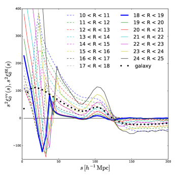
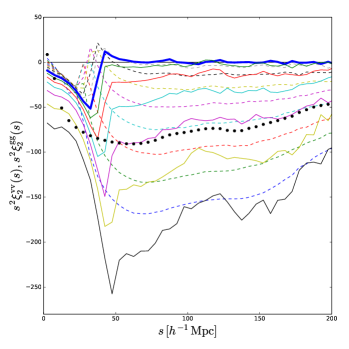
Figure 1: Monopoles and quadrupoles of the auto-correlation functions measured from 100 patchy mock void and galaxy catalogs in boxes with different void radius $R$ bins.

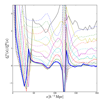
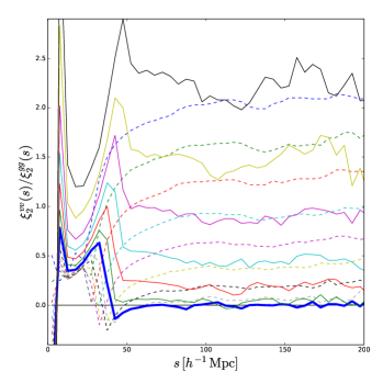
Figure 2: Using the results shown in Fig. 1, we compute the ratios of the monopoles (and quadrupoles) of the voids auto-correlation functions versus the one from galaxy auto-correlation function. We compute $r_{0}$ and $r_{2}$ by averaging the scale range of $[160,200]$ $h^{-1}$ Mpc. The color lines showing different void sizes as described in Fig. 1.

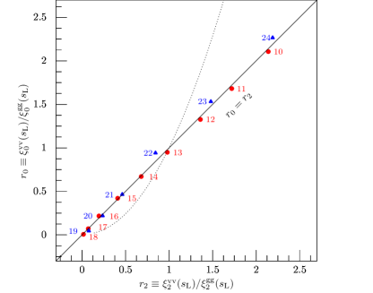
Figure 3: Monopole and quadrupole ratios based on mock catalogs as shown in Fig. 1. The numbers in red and blue indicate the void radius for negative and positive bias, respectively. The void bias $b^{s}_{\rm vg}$ changes sign when $R$ is between 18 and 19 $h^{-1}$ Mpc. We show also the predicion of $r_{0}$ vs $r_{2}$ from the Kaiser approximation (black dotted line). We assume the linear bias of galaxies is 2 and the growth rate at the redshift of the sample is 0.75. One can see that the prediction is very different from $r_{0}=r_{2}$ as observed from our simulations.

We use 100 mock void catalogs (using the dive algorithm, see Ref. (Zhao et al., 2016))) constructed based on mock galaxy catalogues defined in redshift space (using the patchy code, see Ref. (Kitaura et al., 2014)), which resemble the clustering of BOSS Luminous Red Galaxies with number density around $3.5\times 10^{-4}\,h^{3}\,\mathrm{Mpc}^{-3}$, at a mean redshift of $z\simeq 0.56$ in cubical volumes of 2.5 $h^{-1}$Gpc side (described in Ref. (Kitaura et al., 2016)).

We compute monopoles and quadrupoles for void populations with radii ranging from 10 to 25 and bins of 1 $h^{-1}$ Mpc (see in Fig. 1).

We define

$$r_{l} \equiv \frac{\xi^{{\rm v}{\rm v}}_{l}(s_{\rm L})}{\xi^{\rm g\rm g}_{l}(s_{\rm L})}\,,$$ (1)

for the different multipoles $l\in[0,2]$ of the void auto-correlation function ($\xi^{{\rm v}{\rm v}}_{l}$) and galaxy auto-correlation function ($\xi^{\rm g\rm g}_{l}$) with $s_{\rm L}$ defined on large scales. Fig. 2 shows the scale dependency of $r_{0}$ and $r_{2}$.

By computing the averages of the ratios within the scale range of $s_{\rm L}\in[160,200]$ $h^{-1}$ Mpc we get a very good agreement $r_{0}\simeq r_{2}$, as shown in the $r_{0}$-$r_{2}$ scatter plot for different $R$ bins on the left panel in Fig. 3. Note that $r_{0}=r_{2}$ does not agree with the prediction of the Kaiser approximation as shown in Fig. 3. Thus, a different theory, as we develop in the next section, beyond the Kaiser approximation is needed to understand what we observe in this study. We will explain in detail in the next theory section.

III Theory: linear RSD for voids

The relation between the galaxy contrast $\delta_{\rm g}$ and the dark matter field includes nonlinear, nonlocal, and stochastic components (see, e.g., Kaiser, 1984; Coles, 1993; Fry and Gaztanaga, 1993; Bond and Myers, 1996; Dekel and Lahav, 1999; Seljak, 2000; Berlind et al., 2003; McDonald and Roy, 2009; Desjacques et al., 2010; Matsubara, 2011; Schmidt, 2013; Kitaura et al., 2014; Saito et al., 2014; Baldauf et al., 2015), and can be written for long wavelength modes as

$$\delta_{\rm g}(\mbox{\boldmath$r$})=b_{\rm g}\delta(\mbox{\boldmath$r$})+\epsilon_{\rm g}(\mbox{\boldmath$r$})+\cdots\,,$$ (2)

where $b_{\rm g}$ is the linear bias, $\delta(\mbox{\boldmath$r$})$ is the dark matter field, and $\epsilon_{\rm g}$ is the galaxy noise term, followed by nonlinear and nonlocal terms.

The linear bias can be obtained from the measured clustering of galaxies, for instance the power spectrum (the auto-correlation function in Fourier space) at large scales related to the dark matter power spectrum

$$P_{\rm g\rm g}({\mbox{\boldmath$k$}})=b_{\rm g}^{2}\,P({\mbox{\boldmath$k$}})+P_{\epsilon}\,,$$ (3)

with $P({\mbox{\boldmath$k$}})\equiv\langle\overline{\hat{\delta}(\mbox{\boldmath$k$})}\hat{\delta}(\mbox{\boldmath$k$})\rangle$, the dark matter density contrast in Fourier space given by $\hat{\delta}(\mbox{\boldmath$k$})$, and $P_{\epsilon}$ standing for the noise power spectrum.

The action of gravity on large scales causes coherent flows in which galaxies tend to infall into larger density regions contributing to increment the density. This effect produces an enhancement of the power on large scales given by the Kaiser factor (see Ref. (Kaiser, 1987)). Therefore, in redshift space, the galaxy density contrast to linear order is given by

$$\hat{\delta}_{\rm g}^{s}(\mbox{\boldmath$k$}) = \hat{\delta}_{\rm g}(\mbox{\boldmath$k$})+f\mu^{2}\hat{\delta}(\mbox{\boldmath$k$})+\hat{\epsilon}\,,$$ (4)

$$= \left(1+\beta_{\rm g}\mu^{2}\right)\,b_{\rm g}\,\hat{\delta}(\mbox{\boldmath$k$})+\hat{\epsilon}\,,$$ (5)

with $f$ being the logarithmic growth rate, $\beta_{\rm g}\equiv{f}/{b_{\rm g}}$, $\mu=\frac{\mbox{\boldmath$k$}}{k}\cdot\hat{\mbox{\boldmath$r$}}$, and $\hat{\mbox{\boldmath$r$}}$ being the line-of-sight direction. We will refer to the redshift space term $f\mu^{2}\hat{\delta}(\mbox{\boldmath$k$})$ as $\hat{\eta}_{\rm g}(\mbox{\boldmath$k$})$ in Fourier space and ${\eta}_{\rm g}(\mbox{\boldmath$r$})$ in configuration space. Therefore the effective bias relating the galaxy density contrast in redshift space to the dark matter field can be considered to be given by $b^{s}_{\rm g}\equiv\left(1+\beta_{\rm g}\mu^{2}\right)\,b_{\rm g}=b_{\rm g}+f\mu^{2}$. This implies that in this model the bias contribution from RSD is the same as for the dark matter (which is the unbiased case $b_{\rm g}=1$). However, in general this is not true, so that a tracer resulting from a nonlinear transformation of the density field ${\rm T}(\hat{\delta})$ with linear bias $b^{\delta}_{\rm T}$ will introduce a bias in the RSD term $b^{\eta}_{\rm T}$ (see Refs. (Seljak, 2012; McDonald et al., 2000; McDonald, 2003; Wang et al., 2015))

$$b_{\rm T}(\mu)=b^{\delta}_{\rm T}+b^{\eta}_{\rm T}\,(f\mu^{2})\,.$$ (6)

where $b_{\rm T}^{\delta}$ and $b_{\rm T}^{\eta}$ are related to the response of the tracer ${\rm T}$ to small variations of the density and of the line-of-sight velocity gradient, respectively. The $b_{\rm T}^{\eta}$ factor is “one” for galaxies, as their number density is conserved in the real- to redshift-space mapping. This is however, not the case for the Lyman alpha forest or for voids. In fact, some voids disappear or change their size in this mapping procedure (see Ref. (Zhao et al., 2016)).

We must be thus careful when constructing the bias model for voids, as these are equivalent to a nonlinear and nonlocal transformation of the galaxy density field in redshift space.

Voids can be considered to be tracers over an extended region characterized by their radius $R$. Following McDonald and Roy (2009), assuming isotropy and a general short-range non-locality (SRNL) kernel $K$, with the only condition that it must fall to zero outside a typical scale $R$, we can make a Taylor expansion around $\Delta\mbox{\boldmath$r$}=\mbox{\boldmath$r$}-\mbox{\boldmath$r$}^{\prime}$, to find a general expression for the void density contrast in redshift space as a function of the linear galaxy field in redshift space after considering only the leading order term

$$\delta_{\rm v}^{s}\left(\mbox{\boldmath$r$}\right)=\int d\Delta\mbox{\boldmath$r$}K\left(\left|\Delta\mbox{\boldmath$r$}\right|\right)\delta_{\rm g}^{s}(\mbox{\boldmath$r$}+\Delta\mbox{\boldmath$r$})+\epsilon_{\rm v}(\mbox{\boldmath$r$})$$

$$=\int d\Delta\mbox{\boldmath$r$}K(\left|\Delta\mbox{\boldmath$r$}\right|)\left[\delta_{\rm g}^{s}(\mbox{\boldmath$r$})+\frac{d\delta_{\rm g}^{s}(\mbox{\boldmath$r$})}{dr_{i}}\Delta r_{i}\right.$$

$$\hskip 85.35826pt\left.+\frac{1}{2}\frac{d^{2}\delta_{\rm g}^{s}(\mbox{\boldmath$r$})}{dr_{i}dr_{j}}\Delta r_{i}\Delta r_{j}+...\right]+\epsilon_{\rm v}(\mbox{\boldmath$r$})$$

$$=\delta_{\rm g}^{s}(\mbox{\boldmath$r$})\int d\Delta\mbox{\boldmath$r$}K\left(\left|\Delta\mbox{\boldmath$r$}\right|\right)+\frac{d\delta_{\rm g}^{s}(\mbox{\boldmath$r$})}{dr_{i}}\int d\Delta\mbox{\boldmath$r$}K\left(\left|\Delta\mbox{\boldmath$r$}\right|\right)\Delta r_{i}$$

$$\hskip 28.45274pt+\frac{1}{2}\frac{d^{2}\delta_{\rm g}^{s}(\mbox{\boldmath$r$})}{dr_{i}dr_{j}}\int d\Delta\mbox{\boldmath$r$}K\left(\left|\Delta\mbox{\boldmath$r$}\right|\right)\Delta r_{i}\Delta r_{j}+\epsilon_{\rm v}(\mbox{\boldmath$r$})+...\,,$$

where $\epsilon_{\rm v}$ is the void noise term. Note that we have assumed the kernel is isotropic in redshift-space coordinates, which can be made true by construction at a bare (un-renormalized) level. In general SRNL can have some radial-transverse asymmetry in redshift space.

The simple integral over $K$ in the first term is a linear bias $b^{s}_{\rm vg}$; while the 2nd term, integrating $K~{}\Delta r_{i}$, must be zero by the symmetry of the kernel; and the third term, integrating $K~{}\Delta r_{i}\Delta r_{j}$ must be zero by symmetry if $i\neq j$, but if $i=j$, the integral for a generic kernel will give a result of order $R^{2}$ times the simple integral over the kernel in the first term, i.e., the integral will give a result of order $\sim b^{s}_{\rm vg}R^{2}\delta^{K}_{ij}$. Therefore, one gets

$$\delta^{s}_{\rm v}\left(\mbox{\boldmath$r$}\right)=b^{s}_{\rm vg}\left[\delta_{\rm g}\left(\mbox{\boldmath$r$}\right)+\frac{\tilde{b}_{R}}{2}R^{2}\nabla^{2}\delta^{s}_{\rm g}\left(\mbox{\boldmath$r$}\right)\right]+\epsilon_{\rm v}(\mbox{\boldmath$r$})+...$$ (8)

where $\tilde{b}_{R}$ is of order unity (e.g., if the kernel was a Gaussian with root mean square width $R$, $\tilde{b}_{R}$ would be exactly 1), which in Fourier space is written as

$$\hat{\delta}_{\rm vg}^{s}\left(\mbox{\boldmath$k$}\right)=b^{s}_{\rm vg}\left[1-\frac{\tilde{b}_{R}}{2}R^{2}k^{2}\right]\hat{\delta}^{s}_{\rm g}\left(\mbox{\boldmath$k$}\right)+\hat{\epsilon}_{\rm v}(\mbox{\boldmath$k$})+...\,.$$ (9)

This model permits us to assume a linear void bias within a quasi-local approximation in the large scale limit.

Let us therefore consider the case in which voids trace only the linear part of the galaxy field in redshift space

$$\hat{\delta}_{\rm v}^{s}(\mbox{\boldmath$k$}) = b^{s}_{\rm vg}\hat{\delta}_{\rm g}^{s}(\mbox{\boldmath$k$})+\hat{\epsilon}_{\rm v}(\mbox{\boldmath$k$})\,,$$ (10)

$$= b^{s}_{\rm vg}b_{\rm g}\hat{\delta}(\mbox{\boldmath$k$})+b^{s}_{\rm vg}f\mu^{2}\hat{\delta}(\mbox{\boldmath$k$})+\hat{\epsilon}_{\rm v}(\mbox{\boldmath$k$})\,,$$ (11)

$$= (1+\beta_{\rm g}\mu^{2})\,b^{s}_{\rm vg}b_{\rm g}\,\hat{\delta}(\mbox{\boldmath$k$})+\hat{\epsilon}_{\rm v}(\mbox{\boldmath$k$})\,.$$ (12)

This simplified model has two interesting implications. First, that the bias induced by RSD for voids on large scales is given by $b^{s}_{\rm vg}$ and not “one” as for galaxies. Second, that the beta factor $\beta_{\rm g}$ is the same as for galaxies. The key finding of this letter is that this formula seems to describe the results of our simulations, suggesting that the approximations that go into it, i.e., neglecting non-linear effects explored later, are valid.

In this approximation, the multipoles of void power spectra can be expressed by

$$P^{{\rm v}{\rm v}}_{l}(k) = (b^{s}_{\rm vg})^{2}P^{\rm g\rm g}_{l}(k)\,,$$ (13)

and the multipoles of void correlation functions by

$$\xi^{{\rm v}{\rm v}}_{l}(s) = (b^{s}_{\rm vg})^{2}\xi^{\rm g\rm g}_{l}(s)\,,$$ (14)

for multipoles $l\in[0,2,4]$. In addition, the multipoles of void cross-power spectra can be expressed by

$$P^{{\rm v}\rm g}_{l}(k) = b^{s}_{\rm vg}\,P^{\rm g\rm g}_{l}(k)\,,$$ (15)

and the multipoles of void cross-correlation functions by

$$\xi^{{\rm v}\rm g}_{l}(s) = b^{s}_{\rm vg}\,\xi^{\rm g\rm g}_{l}(s)\,,$$ (16)

where we have neglected additional noise terms.

If we consider that voids trace nonlinear galaxy density components we can demonstrate that the beta parameter for voids is not the same as for galaxies. Below is an existence proof but not intended to be taken literally as a prediction.

Let us consider up to second order bias in the galaxy density contrast in redshift space and neglect nonlocal bias terms

$$\delta^{s}_{\rm g}(\mbox{\boldmath$r$})=b^{(1)}_{\rm g}\,\delta(\mbox{\boldmath$r$})+b^{(2)}_{\rm g}\,(\delta^{2}(\mbox{\boldmath$r$})-\sigma^{2})+\eta(\mbox{\boldmath$r$})+\epsilon_{\rm g}(\mbox{\boldmath$r$})\,,$$ (17)

with $\sigma^{2}\equiv\langle\delta^{2}(\mbox{\boldmath$r$})\rangle$, including the RSD term $\eta$.

To get an expression for the linear bias $b_{\rm g}$ one can cross correlate the galaxy field $\delta^{s}_{\rm g}(\mbox{\boldmath$r$})$ with the linear density field $\delta(\mbox{\boldmath$r$})$

$$\langle\delta(\mbox{\boldmath$r$}+{\rm d}\mbox{\boldmath$r$})\delta^{s}_{\rm g}(\mbox{\boldmath$r$})\rangle=b^{(1)}_{\rm g}\,\langle\delta(\mbox{\boldmath$r$}+{\rm d}\mbox{\boldmath$r$})\delta(\mbox{\boldmath$r$})\rangle+\langle\delta(\mbox{\boldmath$r$}+{\rm d}\mbox{\boldmath$r$})\eta(\mbox{\boldmath$r$})\rangle\,.$$ (18)

Since we assume that $\delta$ is Gaussian, the term $\langle\delta(\mbox{\boldmath$r$}+{\rm d}\mbox{\boldmath$r$})\delta^{2}(\mbox{\boldmath$r$})\rangle$ vanishes. The two remaining terms can be expressed in Fourier space as $P(\mbox{\boldmath$k$})\equiv\langle\overline{\hat{\delta}(\mbox{\boldmath$k$})}\hat{\delta}(\mbox{\boldmath$k$})\rangle$ and $f\mu^{2}\,P(\mbox{\boldmath$k$})=\langle\overline{\hat{\delta}(\mbox{\boldmath$k$})}\hat{\eta}(\mbox{\boldmath$k$})\rangle$ yielding hence

$$\langle\overline{\hat{\delta}(\mbox{\boldmath$k$})}\hat{\delta}^{s}_{\rm g}(\mbox{\boldmath$k$})\rangle=b^{(1)}_{\rm g}\,P(\mbox{\boldmath$k$})+f\mu^{2}\,P(\mbox{\boldmath$k$})=(1+\beta_{\rm g}\mu^{2})b^{(1)}_{\rm g}P(\mbox{\boldmath$k$})\,,$$ (19)

with $\beta_{\rm g}\equiv f/b^{(1)}_{\rm g}$ (in our particular formulation $b_{\rm g}=b^{(1)}_{\rm g}$, for a more general case we would need to include third order terms, see Ref. (McDonald, 2006)).

The void density contrast in redshift space can be written to third order bias as by neglecting for the sake of simplicity the convolution kernel $K$ as

$$\delta^{s}_{\rm v}(\mbox{\boldmath$r$})=b^{s(1)}_{\rm vg}\,\delta^{s}_{\rm g}(\mbox{\boldmath$r$})+b^{s(2)}_{\rm vg}\,((\delta^{s}_{\rm g}(\mbox{\boldmath$r$}))^{2}-\sigma_{s}^{2})+b^{s(3)}_{\rm vg}\,(\delta^{s}_{\rm g}(\mbox{\boldmath$r$}))^{3}+\epsilon_{\rm v}(\mbox{\boldmath$r$})\,,$$ (20)

with $\sigma_{s}^{2}\equiv\langle(\delta^{s}_{\rm g}(\mbox{\boldmath$r$}))^{2}\rangle$, $\epsilon_{\rm v}$ being the voids shot noise.

By cross-correlating with the dark matter density contrast up to second order we get

$$\langle{\delta}(\mbox{\boldmath$r$}+{\rm d}\mbox{\boldmath$r$}){\delta}^{s}_{\rm v}(\mbox{\boldmath$r$})\rangle$$

$$=b^{s(1)}_{\rm vg}\langle{\delta}(\mbox{\boldmath$r$}+{\rm d}\mbox{\boldmath$r$}){\delta}^{s}_{\rm g}(\mbox{\boldmath$r$})\rangle+b^{s(2)}_{\rm vg}\langle{\delta}(\mbox{\boldmath$r$}+{\rm d}\mbox{\boldmath$r$})({\delta}^{s}_{\rm g}(\mbox{\boldmath$r$}))^{2}\rangle$$

$$=b^{s(1)}_{\rm vg}b^{(1)}_{\rm g}\langle{\delta}(\mbox{\boldmath$r$}+{\rm d}\mbox{\boldmath$r$}){\delta}(\mbox{\boldmath$r$})\rangle+b^{s(1)}_{\rm vg}\langle{\delta}(\mbox{\boldmath$r$}+{\rm d}\mbox{\boldmath$r$}){\eta}(\mbox{\boldmath$r$})\rangle$$

$$+2b^{s(2)}_{\rm vg}b^{(1)}_{\rm g}b^{(2)}_{\rm g}\langle{\delta}(\mbox{\boldmath$r$}+{\rm d}\mbox{\boldmath$r$})\delta(\mbox{\boldmath$r$})(\delta(\mbox{\boldmath$r$})^{2}-\sigma^{2})\rangle$$

$$+2b^{s(2)}_{\rm vg}b^{(2)}_{\rm g}\langle{\delta}(\mbox{\boldmath$r$}+{\rm d}\mbox{\boldmath$r$})(\delta(\mbox{\boldmath$r$})^{2}-\sigma^{2})\eta(\mbox{\boldmath$r$})\rangle\,,$$

where we have used that $\langle\delta(\mbox{\boldmath$r$}+{\rm d}\mbox{\boldmath$r$})\epsilon_{\rm v}(\mbox{\boldmath$r$})\rangle=0$ and the fact that the expected value of terms with an odd number of Gaussian variables is zero.

Using Wick’s theorem we can write this in Fourier space as

$$\langle\overline{\hat{\delta}(\mbox{\boldmath$k$})}\hat{\delta}^{s}_{\rm v}(\mbox{\boldmath$k$})\rangle$$

$$=b^{s(1)}_{\rm vg}(b^{(1)}_{\rm g}+f\mu^{2})P(\mbox{\boldmath$k$})+4b^{s(2)}_{\rm vg}b^{(2)}_{\rm g}(b^{(1)}_{\rm g}\sigma^{2}+\sigma_{\delta\eta}^{2})P(\mbox{\boldmath$k$})\,,$$

where $\sigma^{2}_{\delta\eta}\equiv\langle{\delta}(\mbox{\boldmath$r$})\eta(\mbox{\boldmath$r$})\rangle$, i.e., the zero-lag correlation of the linear density and the gradient of the velocity field.

We can compress the above cross correlation expression to

$${\langle\overline{\hat{\delta}(\mbox{\boldmath$k$})}\hat{\delta}^{s}_{\rm v}(\mbox{\boldmath$k$})\rangle}=(1+\beta_{\rm v}\mu^{2})b^{s}_{\rm v}P(\mbox{\boldmath$k$})\,,$$ (23)

by introducing an effective void bias

$$b^{s}_{\rm v}\equiv b^{s(1)}_{\rm vg}b^{(1)}_{\rm g}+4b^{s(2)}_{\rm vg}b^{(2)}_{\rm g}(b^{(1)}_{\rm g}\sigma^{2}+\sigma_{\delta\eta}^{2})\,,$$ (24)

and defining a new void beta factor

$$\beta_{\rm v}\equiv\frac{b^{s(1)}_{\rm vg}}{b^{s}_{\rm v}}f=\frac{b^{s(1)}_{\rm vg}}{b^{s(1)}_{\rm vg}b^{(1)}_{\rm g}+4b^{s(2)}_{\rm vg}b^{(2)}_{\rm g}(b^{(1)}_{\rm g}\sigma^{2}+\sigma_{\delta\eta}^{2})}f\,.$$ (25)

From this equation we can see that we will only have $\beta_{v}=\beta_{g}=f/b_{g}^{(1)}$ in the spacial case that voids are tracing the linear galaxy redshift space field, i.e., when $b^{(2)}_{\rm g}=0$.

In fact, as long as voids trace only the linear galaxy redshift space field, the beta parameter equality between voids and galaxies is also ensured with more complex higher order relations.​ If we include higher order terms in the voids galaxy relation, up to third order, and compute its cross correlation with the linear density field we get

$$\langle{\delta}(\mbox{\boldmath$r$}+{\rm d}\mbox{\boldmath$r$}){\delta}^{s}_{\rm v}(\mbox{\boldmath$r$})\rangle$$

$$=b^{s(1)}_{\rm vg}\langle{\delta}(\mbox{\boldmath$r$}+{\rm d}\mbox{\boldmath$r$}){\delta}^{s}_{\rm g}(\mbox{\boldmath$r$})\rangle+b^{s(3)}_{\rm vg}\langle{\delta}(\mbox{\boldmath$r$}+{\rm d}\mbox{\boldmath$r$})({\delta}^{s}_{\rm g}(\mbox{\boldmath$r$}))^{3}\rangle\,,$$

where we have used that $\langle\delta(\mbox{\boldmath$r$}+{\rm d}\mbox{\boldmath$r$})\epsilon_{\rm v}(\mbox{\boldmath$r$})\rangle=0$ and $\langle\delta(\mbox{\boldmath$r$}+{\rm d}\mbox{\boldmath$r$})(\delta^{s}_{\rm g}(\mbox{\boldmath$r$}))^{2}\rangle=0$, since $\delta^{s}_{\rm g}(\mbox{\boldmath$r$})$ is also a Gaussian field.

Expanding the second term in Eq. III we find

$$\langle{\delta}(\mbox{\boldmath$r$}+{\rm d}\mbox{\boldmath$r$})({\delta}^{s}_{\rm g}(\mbox{\boldmath$r$}))^{3}\rangle$$

$$=b^{(1)}_{\rm g}\langle{\delta}(\mbox{\boldmath$r$}+{\rm d}\mbox{\boldmath$r$})({\delta}(\mbox{\boldmath$r$}))^{3}\rangle+\langle{\delta}(\mbox{\boldmath$r$}+{\rm d}\mbox{\boldmath$r$})({\eta}(\mbox{\boldmath$r$}))^{3}\rangle$$

$$+3(b^{(1)}_{\rm g})^{2}\langle{\delta}(\mbox{\boldmath$r$}+{\rm d}\mbox{\boldmath$r$})({\delta}(\mbox{\boldmath$r$}))^{2}\eta(\mbox{\boldmath$r$})\rangle$$

$$+3(b^{(1)}_{\rm g})^{2}\langle{\delta}(\mbox{\boldmath$r$}+{\rm d}\mbox{\boldmath$r$}){\delta}(\mbox{\boldmath$r$})(\eta(\mbox{\boldmath$r$}))^{2}\rangle$$

$$+3(b^{(1)}_{\rm g})^{2}\langle{\delta}(\mbox{\boldmath$r$}+{\rm d}\mbox{\boldmath$r$}){\delta}(\mbox{\boldmath$r$})(\epsilon(\mbox{\boldmath$r$}))^{2}\rangle$$

$$+3(b^{(1)}_{\rm g})^{2}\langle{\delta}(\mbox{\boldmath$r$}+{\rm d}\mbox{\boldmath$r$}){\eta}(\mbox{\boldmath$r$})(\epsilon(\mbox{\boldmath$r$}))^{2}\rangle\,,$$

which in Fourier space reduces to

$$=3(b^{(1)}_{\rm g})^{2}\sigma_{\delta\delta}^{2}P(k)+3\sigma_{\eta\eta}f\mu^{2}P(k)+3(b^{(1)}_{\rm g})^{2}\sigma_{\delta\delta}^{2}f\mu^{2}P(k)$$

$$+6(b^{(1)}_{\rm g})^{2}\sigma_{\delta\eta}^{2}P(k)+3b^{(1)}_{\rm g}\sigma_{\eta\eta}^{2}P(k)+6b^{(1)}_{\rm g}\sigma_{\delta\eta}^{2}f\mu^{2}P(k)$$

$$+3b^{(1)}_{\rm g}\sigma_{\epsilon\epsilon}^{2}P(k)+3\sigma_{\epsilon\epsilon}^{2}f\mu^{2}P(k)$$

$$=3[(b^{(1)}_{\rm g})^{3}\sigma_{\delta\delta}^{2}+2(b^{(1)}_{\rm g})^{2}\sigma_{\delta\eta}^{2}+b^{(1)}_{\rm g}\sigma_{\eta\eta}^{2}+b^{(1)}_{\rm g}\sigma_{\epsilon\epsilon}^{2}]P(k)$$

$$+3[\sigma_{\eta\eta}^{2}+(b^{(1)}_{\rm g})^{2}\sigma_{\delta\delta}^{2}+2b^{(1)}_{\rm g}\sigma_{\delta\eta}^{2}+\sigma_{\epsilon\epsilon}]f\mu^{2}P(k)$$

$$=3[\sigma_{\eta\eta}^{2}+(b^{(1)}_{\rm g})^{2}\sigma_{\delta\delta}^{2}+2b^{(1)}_{\rm g}\sigma_{\delta\eta}^{2}+\sigma_{\epsilon\epsilon}][b^{(1)}_{\rm g}+f\mu^{2}]P(k)\,,$$

Combining this result with the first term of Eq. III we get

$${\overline{\langle\hat{\delta}(\mbox{\boldmath$k$})}\hat{\delta}^{s}_{\rm v}(\mbox{\boldmath$k$})\rangle=\tilde{b}[b^{(1)}_{\rm g}+f\mu^{2}]P(k)}\,,$$ (28)

with $\tilde{b}\equiv b^{s(1)}_{\rm vg}+3b^{s(3)}_{\rm vg}[\sigma_{\eta\eta}^{2}+(b^{(1)}_{\rm g})^{2}\sigma_{\delta\delta}^{2}+2b^{(1)}_{\rm g}\sigma_{\delta\eta}^{2}+\sigma_{\epsilon\epsilon}]$. From this we can conclude that even a non-linear transformation up to third order of the linear galaxy redshift space will retain the same beta factor: $\beta_{\rm v}=\beta_{\rm g}=f/b^{(1)}_{\rm g}$.

IV Validation of the RSD void model

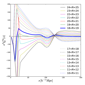
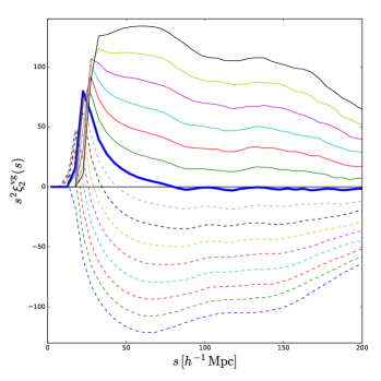
Figure 4: Monopoles and quadrupoles the cross-correlation functions measured from 100 patchy mock void and galaxy catalogs in boxes with different void radius $R$ bins.

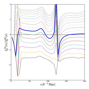
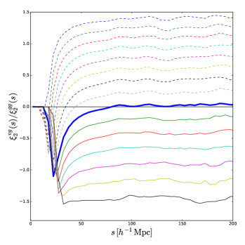
Figure 5: Using the results shown in Fig. 4, we compute the ratios of the monopoles (and quadrupoles) of the void-galaxy cross-correlation functions versus the one from galaxy auto-correlation function. The color lines showing different void sizes as described in Fig. 4.

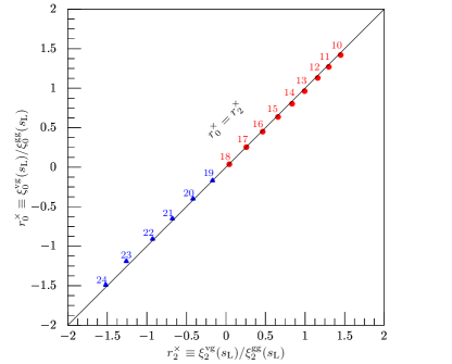
Figure 6: Monopole and quadrupole ratios based on mock catalogs as shown in Fig. 5. The numbers in red and blue indicate the void radius for negative and positive bias, respectively. The void bias $b^{s}_{\rm vg}$ changes sign when $R$ is between 18 and 19 $h^{-1}$ Mpc.

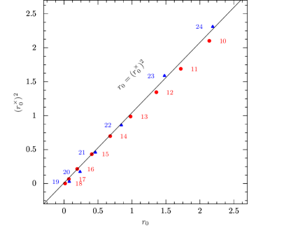
Figure 7: $(r^{\times}_{0})^{2}$ vs $r_{0}$. The notations are the same as the ones in Fig. 3 and Fig. 6. The numbers in red and blue indicate the void radius for negative and positive bias respectively. The results agree with our prediction, $(r^{\times}_{0})^{2}=r_{0}=(b^{s}_{\rm vg})^{2}$. However, we see also slight deviation for smaller voids, e.g. $10<R<11$ $h^{-1}$ Mpc. It should be due to the fact that smaller voids are no longer tracing only the linear galaxy density field in redshift space.

One can verify whether voids are tracing only the linear galaxy redshift space field from the multipoles of the correlation function as we have shown above, since the ratio between the void-void and the galaxy-galaxy multipoles should yield a constant value in case voids share the same beta factor as galaxies.

To reassure, we compute also the cross-correlation functions between voids and galaxeis and define the ratio between the void-galaxy and the galaxy-galaxy multipoles

$$r^{\times}_{l} \equiv \frac{\xi^{{\rm v}{\rm g}}_{l}(s_{\rm L})}{\xi^{\rm g\rm g}_{l}(s_{\rm L})}\,,$$ (29)

as shown in Fig. 4 and Fig. 5

For the particular case in which voids are tracers of the linear galaxy redshift space field $r_{l}=(b^{s}_{\rm vg})^{2}$ and $r^{\times}_{l}=b^{s}_{\rm vg}$.

The void-galaxy cross-correlation function relations lead to a very good agreement $r^{\times}_{0}\simeq r^{\times}_{2}$ as shown in Fig. 6. We check also the relation between $r_{0}$ and $r^{\times}_{0}$ in Fig. 7 and find it agrees with our prediction, $(r^{\times}_{0})^{2}=r_{0}=(b^{s}_{\rm vg})^{2}$. We see slight deviation for smaller voids, e.g. $10<R<11$ $h^{-1}$ Mpc. It should be due to the fact that smaller voids are no longer tracing only the linear galaxy density field in redshift space.

V Discussion and Summary

We have found that cosmic voids will in general have a beta factor different from the galaxy one. Our results based on mock void catalogs showed void beta factors being in good agreement with the galaxy one indicating that they can be approximately assumed to be quasi-local transformations of the linear galaxy redshift space field.

We introduced the SRNL kernel, i.e., Eq. III, for a specific purpose: In Fig. 4 we see a population of voids that appears to have zero bias in the large-separation limit; however, they nevertheless have a BAO feature, and in fact we have found that a zero bias population can be very good for measuring BAO (Kitaura et al., 2016). Since BAO are a feature of the linear power spectrum, it is surprising that they appear even for a zero-bias population, so this should be understood before these voids are trusted for a distance measurement. One possibility is that the BAO feature comes from non-linearity, but another, probably more compelling possibility is that we have a special case of SRNL. As we saw above, picking a population with zero large-scale bias amounts to tuning the integral over the SRNL kernel to be zero. However, this does not rule out, e.g., a compensated, upside-down Mexican hat-type kernel, i.e., one that favors the presence of a void when the density is low in the center and high at some typical radius. The linear correlation function will then appear convolved with this kernel – wherever it is smooth we will see zero, but where there is a feature like BAO on the scale of the kernel the correlation will be non-zero (e.g., for a delta function feature, the result will just look like the kernel), similar to what we see in Fig. 4. Plots of the mean mass as a function of the distance from void centers, which are closely related to this kernel, also look very consistent with this understanding Zhao et al. (2016).

Appendix A Particular case: zero bias voids

In this section we use data from the Data Release DR11 (see Ref. (Alam et al., 2015b)) of the Baryon Oscillation Spectroscopic Survey (BOSS, see Ref. (Eisenstein et al., 2011)). The BOSS survey uses the SDSS 2.5 meter telescope at Apache Point Observatory (see Ref. (Gunn et al., 2006)) and the spectra are obtained using the double-armed BOSS spectrograph (see Ref. (Smee et al., 2013)). The data are then reduced using the algorithms described in (Bolton et al., 2012). The target selection of the CMASS and LOWZ samples, together with the algorithms used to create large scale structure catalogs (the mksample code), are presented in Ref. (Reid and et al., 2016).

We restrict this analysis to the CMASS sample of luminous red galaxies (LRGs), which is a complete sample, nearly constant in mass and volume limited between the redshifts $0.43\leq z\leq 0.7$ (see (Reid and et al., 2016; Anderson and et al., 2014) for details of the targeting strategy).

Based on the mock galaxy catalogs for the CMASS sample (see Ref. (Kitaura et al. et al., 2016; Rodríguez-Torres et al., 2015)) and on the void catalog obtained with the dive code (see Ref. (Zhao et al., 2016)) we compute the quadrupoles for the void population selected with a radius cut of 16 $h^{-1}$ Mpc (see Fig. 9). This is the population leading to the largest BAO signal-to-noise ratio without further considering optimal weights (see Ref. (Liang et al., 2016)) used to measure the BAO from CMASS BOSS DR11 data (see Ref. (Kitaura et al., 2016)). We find a closely vanishing quadrupole at large scales. We see a similar behavior from DR11 patchy mock catalogs.

In Fig. 8 we can see that the 2D correlation functions from the observed void catalog is as compared to the galaxies. We find that the correlation function vanishes on large scales, as expected for zero bias tracers. This particular case gives further support to the void bias model being tracer of the linear galaxy redshift space field.

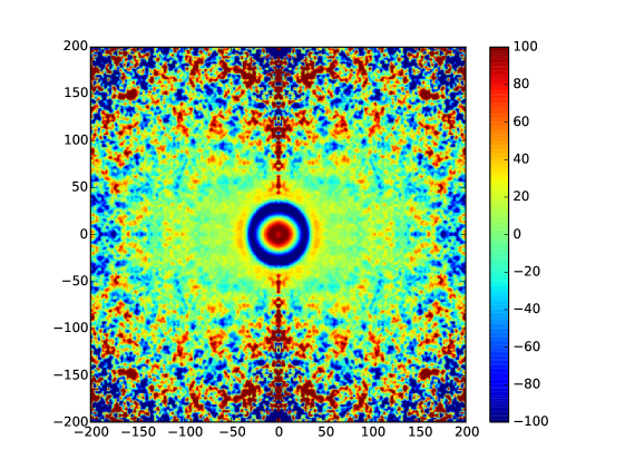
Figure 8: 2D correlation function for CMASS DR11 left panel: voids; right panel: galaxies.

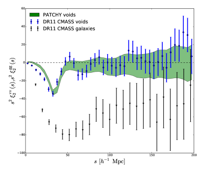
Figure 9: Quadrupoles of void correlation functions from CMASS-NGC DR11 voids (blue points) and the averaged correlation function from 1000 patchy mock void catalogs (green area indicates the 1 $\sigma$ region). Black dots and error bars: quadrupole from the CMASS DR11 galaxy clustering.

References

- Alcock and Paczynski (1979) C. Alcock and B. Paczynski, Nature (London) 281, 358 (1979).
- Sachs and Wolfe (1967) R. K. Sachs and A. M. Wolfe, Astrophys. J. 147, 73 (1967).
- Granett et al. (2008) B. R. Granett, M. C. Neyrinck, and I. Szapudi, ApJ 683, L99 (2008), arXiv:0805.3695 .
- Lee and Park (2009) J. Lee and D. Park, ApJ 696, L10 (2009), arXiv:0704.0881 .
- Betancort-Rijo et al. (2009) J. Betancort-Rijo, S. G. Patiri, F. Prada, and A. E. Romano, MNRAS 400, 1835 (2009), arXiv:0901.1609 .
- Lavaux and Wandelt (2012) G. Lavaux and B. D. Wandelt, Astrophys. J. 754, 109 (2012), arXiv:1110.0345 [astro-ph.CO] .
- Bos et al. (2012) E. G. P. Bos, R. van de Weygaert, K. Dolag, and V. Pettorino, MNRAS 426, 440 (2012), arXiv:1205.4238 [astro-ph.CO] .
- Clampitt et al. (2013) J. Clampitt, Y.-C. Cai, and B. Li, MNRAS 431, 749 (2013), arXiv:1212.2216 [astro-ph.CO] .
- Higuchi et al. (2013) Y. Higuchi, M. Oguri, and T. Hamana, MNRAS 432, 1021 (2013), arXiv:1211.5966 .
- Krause et al. (2013) E. Krause, T.-C. Chang, O. Doré, and K. Umetsu, ApJ 762, L20 (2013), arXiv:1210.2446 .
- Sutter et al. (2014) P. M. Sutter, A. Pisani, B. D. Wandelt, and D. H. Weinberg, MNRAS 443, 2983 (2014), arXiv:1404.5618 .
- Cai et al. (2014a) Y.-C. Cai, B. Li, S. Cole, C. S. Frenk, and M. Neyrinck, MNRAS 439, 2978 (2014a), arXiv:1310.6986 [astro-ph.CO] .
- Cai et al. (2014b) Y.-C. Cai, M. C. Neyrinck, I. Szapudi, S. Cole, and C. S. Frenk, Astrophys. J. 786, 110 (2014b), arXiv:1301.6136 .
- Cai et al. (2015) Y.-C. Cai, N. Padilla, and B. Li, MNRAS 451, 1036 (2015), arXiv:1410.1510 .
- Lam et al. (2015) T. Y. Lam, J. Clampitt, Y.-C. Cai, and B. Li, MNRAS 450, 3319 (2015), arXiv:1408.5338 .
- Zivick et al. (2015) P. Zivick, P. M. Sutter, B. D. Wandelt, B. Li, and T. Y. Lam, MNRAS 451, 4215 (2015), arXiv:1411.5694 .
- Barreira et al. (2015) A. Barreira, B. Li, E. Jennings, J. Merten, L. King, C. M. Baugh, and S. Pascoli, MNRAS 454, 4085 (2015), arXiv:1505.03468 .
- Clampitt and Jain (2015) J. Clampitt and B. Jain, MNRAS 454, 3357 (2015), arXiv:1404.1834 .
- Yang et al. (2015) L. F. Yang, M. C. Neyrinck, M. A. Aragón-Calvo, B. Falck, and J. Silk, MNRAS 451, 3606 (2015), arXiv:1411.5029 .
- Gruen et al. (2016) D. Gruen et al., MNRAS 455, 3367 (2016), arXiv:1507.05090 .
- Pollina et al. (2016) G. Pollina, M. Baldi, F. Marulli, and L. Moscardini, MNRAS 455, 3075 (2016), arXiv:1506.08831 .
- Mao et al. (2016) Q. Mao, A. A. Berlind, R. J. Scherrer, M. C. Neyrinck, R. Scoccimarro, J. L. Tinker, and C. K. McBride, ArXiv e-prints (2016), arXiv:1602.06306 .
- White (1979) S. D. M. White, MNRAS 186, 145 (1979).
- Politzer and Preskill (1986) H. D. Politzer and J. P. Preskill, Physical Review Letters 56, 99 (1986).
- Betancort-Rijo (1990) J. Betancort-Rijo, MNRAS 246, 608 (1990).
- Kitaura et al. (2016) F.-S. Kitaura, C.-H. Chuang, Y. Liang, C. Zhao, C. Tao, S. Rodríguez-Torres, D. J. Eisenstein, H. Gil-Marín, J.-P. Kneib, C. McBride, W. J. Percival, A. J. Ross, A. G. Sánchez, J. Tinker, R. Tojeiro, M. Vargas-Magana, and G.-B. Zhao, Physical Review Letters 116, 171301 (2016).
- Liang et al. (2016) Y. Liang, C. Zhao, C.-H. Chuang, F.-S. Kitaura, and C. Tao, MNRAS 459, 4020 (2016), arXiv:1511.04391 .
- Sheth and van de Weygaert (2004) R. K. Sheth and R. van de Weygaert, MNRAS 350, 517 (2004), astro-ph/0311260 .
- Hamaus et al. (2015) N. Hamaus, P. M. Sutter, G. Lavaux, and B. D. Wandelt, J.Cosm.Astr.Phys. 11, 036 (2015), arXiv:1507.04363 .
- Wojtak et al. (2016) R. Wojtak, D. Powell, and T. Abel, MNRAS 458, 4431 (2016), arXiv:1602.08541 .
- Kaiser (1987) N. Kaiser, MNRAS 227, 1 (1987).
- Hamilton (1992) A. J. S. Hamilton, ApJ 385, L5 (1992).
- Cole et al. (1994) S. Cole, K. B. Fisher, and D. H. Weinberg, MNRAS 267, 785 (1994), astro-ph/9308003 .
- Cole et al. (1995) S. Cole, K. B. Fisher, and D. H. Weinberg, MNRAS 275, 515 (1995), astro-ph/9412062 .
- Peacock et al. (2001) J. A. Peacock et al., Nature (London) 410, 169 (2001), astro-ph/0103143 .
- Scoccimarro (2004) R. Scoccimarro, Phys. Rev. D 70, 083007 (2004), astro-ph/0407214 .
- Guzzo et al. (2008) L. Guzzo, M. Pierleoni, B. Meneux, E. Branchini, O. Le Fèvre, C. Marinoni, B. Garilli, J. Blaizot, and et al, Nature (London) 451, 541 (2008), arXiv:0802.1944 .
- Matsubara (2008) T. Matsubara, Phys. Rev. D 78, 083519 (2008), arXiv:0807.1733 .
- Taruya et al. (2009) A. Taruya, T. Nishimichi, S. Saito, and T. Hiramatsu, Phys. Rev. D 80, 123503 (2009), arXiv:0906.0507 [astro-ph.CO] .
- Percival and White (2009) W. J. Percival and M. White, MNRAS 393, 297 (2009), arXiv:0808.0003 .
- Taruya et al. (2010) A. Taruya, T. Nishimichi, and S. Saito, Phys. Rev. D 82, 063522 (2010), arXiv:1006.0699 .
- Seljak and McDonald (2011) U. Seljak and P. McDonald, J.Cosm.Astr.Phys. 11, 039 (2011), arXiv:1109.1888 .
- Jennings et al. (2011) E. Jennings, C. M. Baugh, and S. Pascoli, MNRAS 410, 2081 (2011), arXiv:1003.4282 [astro-ph.CO] .
- Gil-Marín et al. (2012) H. Gil-Marín, C. Wagner, L. Verde, C. Porciani, and R. Jimenez, J.Cosm.Astr.Phys. 11, 029 (2012), arXiv:1209.3771 [astro-ph.CO] .
- Beutler et al. (2012) F. Beutler, C. Blake, M. Colless, D. H. Jones, L. Staveley-Smith, G. B. Poole, L. Campbell, Q. Parker, W. Saunders, and F. Watson, MNRAS 423, 3430 (2012), arXiv:1204.4725 .
- Reid et al. (2012) B. A. Reid et al., MNRAS 426, 2719 (2012), arXiv:1203.6641 .
- Blake et al. (2012) C. Blake et al., MNRAS 425, 405 (2012), arXiv:1204.3674 .
- Okumura et al. (2012) T. Okumura, U. Seljak, P. McDonald, and V. Desjacques, J.Cosm.Astr.Phys. 2, 010 (2012), arXiv:1109.1609 .
- de la Torre and Guzzo (2012) S. de la Torre and L. Guzzo, MNRAS 427, 327 (2012), arXiv:1202.5559 .
- Valageas et al. (2013) P. Valageas, T. Nishimichi, and A. Taruya, Phys. Rev. D 87, 083522 (2013), arXiv:1302.4533 [astro-ph.CO] .
- Chuang and Wang (2013a) C.-H. Chuang and Y. Wang, MNRAS 431, 2634 (2013a), arXiv:1205.5573 .
- Chuang and Wang (2013b) C.-H. Chuang and Y. Wang, MNRAS 435, 255 (2013b), arXiv:1209.0210 .
- Chuang et al. (2013) C.-H. Chuang, F. Prada, A. J. Cuesta, D. J. Eisenstein, E. Kazin, N. Padmanabhan, A. G. Sánchez, X. Xu, and et al, MNRAS 433, 3559 (2013), arXiv:1303.4486 .
- Chuang et al. (2016) C.-H. Chuang, F. Prada, M. Pellejero-Ibanez, F. Beutler, A. J. Cuesta, D. J. Eisenstein, S. Escoffier, S. Ho, and et al, MNRAS 461, 3781 (2016), arXiv:1312.4889 .
- de la Torre et al. (2013) S. de la Torre et al., Astr.Astrophy. 557, A54 (2013), arXiv:1303.2622 .
- Samushia et al. (2014) L. Samushia et al., MNRAS 439, 3504 (2014), arXiv:1312.4899 .
- Howlett et al. (2015) C. Howlett, A. J. Ross, L. Samushia, W. J. Percival, and M. Manera, MNRAS 449, 848 (2015), arXiv:1409.3238 .
- Reid et al. (2014) B. A. Reid, H.-J. Seo, A. Leauthaud, J. L. Tinker, and M. White, MNRAS 444, 476 (2014), arXiv:1404.3742 .
- Okumura et al. (2015) T. Okumura, N. Hand, U. Seljak, Z. Vlah, and V. Desjacques, Phys. Rev. D 92, 103516 (2015), arXiv:1506.05814 .
- Okumura et al. (2016) T. Okumura et al., Publ. Astron. Soc. Jap. 68, 24 (2016), arXiv:1511.08083 [astro-ph.CO] .
- Alam et al. (2015a) S. Alam, S. Ho, M. Vargas-Magaña, and D. P. Schneider, MNRAS 453, 1754 (2015a), arXiv:1504.02100 .
- Wang (2014) Y. Wang, MNRAS 443, 2950 (2014), arXiv:1404.5589 .
- Shoji and Lee (2012) M. Shoji and J. Lee, ArXiv e-prints (2012), arXiv:1203.0869 [astro-ph.CO] .
- Paz et al. (2013) D. Paz, M. Lares, L. Ceccarelli, N. Padilla, and D. G. Lambas, MNRAS 436, 3480 (2013), arXiv:1306.5799 .
- Hamaus et al. (2016) N. Hamaus, A. Pisani, P. M. Sutter, G. Lavaux, S. Escoffier, B. D. Wandelt, and J. Weller, Phys. Rev. Lett. 117, 091302 (2016), arXiv:1602.01784 [astro-ph.CO] .
- Cai et al. (2016) Y.-C. Cai, A. Taylor, J. A. Peacock, and N. Padilla, (2016), 10.1093/mnras/stw1809, arXiv:1603.05184 [astro-ph.CO] .
- Achitouv and Blake (2016) I. Achitouv and C. Blake, (2016), arXiv:1606.03092 [astro-ph.CO] .
- Seljak (2012) U. Seljak, J.Cosm.Astr.Phys. 3, 004 (2012), arXiv:1201.0594 .
- McDonald et al. (2000) P. McDonald, J. Miralda-Escudé, M. Rauch, W. L. W. Sargent, T. A. Barlow, R. Cen, and J. P. Ostriker, Astrophys. J. 543, 1 (2000), astro-ph/9911196 .
- McDonald (2003) P. McDonald, Astrophys. J. 585, 34 (2003), astro-ph/0108064 .
- Wang et al. (2015) X. Wang, A. Font-Ribera, and U. Seljak, J.Cosm.Astr.Phys. 4, 009 (2015), arXiv:1412.4727 .
- Kaiser (1984) N. Kaiser, ApJ 284, L9 (1984).
- Coles (1993) P. Coles, MNRAS 262, 1065 (1993).
- Fry and Gaztanaga (1993) J. N. Fry and E. Gaztanaga, Astrophys. J. 413, 447 (1993), astro-ph/9302009 .
- Bond and Myers (1996) J. R. Bond and S. T. Myers, Rev.Astr.Astrphys. 103, 63 (1996).
- Dekel and Lahav (1999) A. Dekel and O. Lahav, Astrophys. J. 520, 24 (1999), astro-ph/9806193 .
- Seljak (2000) U. Seljak, MNRAS 318, 203 (2000), astro-ph/0001493 .
- Berlind et al. (2003) A. A. Berlind, D. H. Weinberg, A. J. Benson, C. M. Baugh, S. Cole, R. Davé, C. S. Frenk, A. Jenkins, N. Katz, and C. G. Lacey, Astrophys. J. 593, 1 (2003), astro-ph/0212357 .
- McDonald and Roy (2009) P. McDonald and A. Roy, J.Cosm.Astr.Phys. 8, 020 (2009), arXiv:0902.0991 [astro-ph.CO] .
- Desjacques et al. (2010) V. Desjacques, M. Crocce, R. Scoccimarro, and R. K. Sheth, Phys. Rev. D 82, 103529 (2010), arXiv:1009.3449 [astro-ph.CO] .
- Matsubara (2011) T. Matsubara, Phys. Rev. D 83, 083518 (2011), arXiv:1102.4619 [astro-ph.CO] .
- Schmidt (2013) F. Schmidt, Phys. Rev. D 87, 123518 (2013), arXiv:1304.1817 [astro-ph.CO] .
- Kitaura et al. (2014) F.-S. Kitaura, G. Yepes, and F. Prada, MNRAS 439, L21 (2014), arXiv:1307.3285 .
- Saito et al. (2014) S. Saito, T. Baldauf, Z. Vlah, U. Seljak, T. Okumura, and P. McDonald, Phys. Rev. D 90, 123522 (2014), arXiv:1405.1447 .
- Baldauf et al. (2015) T. Baldauf, L. Mercolli, and M. Zaldarriaga, Phys. Rev. D 92, 123007 (2015), arXiv:1507.02256 .
- Zhao et al. (2016) C. Zhao, C. Tao, Y. Liang, F.-S. Kitaura, and C.-H. Chuang, Mon. Not. Roy. Astron. Soc. 459, 2670 (2016), arXiv:1511.04299 [astro-ph.CO] .
- McDonald (2006) P. McDonald, Phys. Rev. D 74, 103512 (2006), astro-ph/0609413 .
- Alam et al. (2015b) S. Alam, F. D. Albareti, C. Allende Prieto, F. Anders, S. F. Anderson, T. Anderton, B. H. Andrews, E. Armengaud, É. Aubourg, S. Bailey, and et al., Rev.Astr.Astrphys. 219, 12 (2015b), arXiv:1501.00963 [astro-ph.IM] .
- Eisenstein et al. (2011) D. J. Eisenstein, D. H. Weinberg, E. Agol, H. Aihara, C. Allende Prieto, S. F. Anderson, J. A. Arns, É. Aubourg, S. Bailey, E. Balbinot, and et al., AJ 142, 72 (2011), arXiv:1101.1529 [astro-ph.IM] .
- Gunn et al. (2006) J. E. Gunn, W. A. Siegmund, E. J. Mannery, R. E. Owen, C. L. Hull, R. F. Leger, L. N. Carey, G. R. Knapp, and et al.,, AJ 131, 2332 (2006), arXiv:astro-ph/0602326 .
- Smee et al. (2013) S. A. Smee, J. E. Gunn, A. Uomoto, N. Roe, D. Schlegel, C. M. Rockosi, M. A. Carr, F. Leger, and et al., AJ 146, 32 (2013), arXiv:1208.2233 [astro-ph.IM] .
- Bolton et al. (2012) A. S. Bolton, D. J. Schlegel, É. Aubourg, S. Bailey, V. Bhardwaj, J. R. Brownstein, S. Burles, Y.-M. Chen, and et al., AJ 144, 144 (2012), arXiv:1207.7326 .
- Reid and et al. (2016) B. Reid and et al., MNRAS 455, 1553 (2016), arXiv:1509.06529 .
- Anderson and et al. (2014) L. Anderson and et al., MNRAS 441, 24 (2014), arXiv:1312.4877 .
- Kitaura et al. et al. (2016) F.-S. Kitaura et al., S. Rodríguez-Torres, C.-H. Chuang, C. Zhao, and et al., MNRAS 456, 4156 (2016), arXiv:1509.06400 .
- Rodríguez-Torres et al. (2015) S. A. Rodríguez-Torres et al., (2015), 10.1093/mnras/stw1014, arXiv:1509.06404 [astro-ph.CO] .