At the survey limits: discovery of the Aquarius 2 dwarf galaxy in the VST ATLAS and the SDSS data

Abstract

We announce the discovery of the Aquarius 2 dwarf galaxy, a new distant satellite of the Milky Way, detected on the fringes of the VST ATLAS and the SDSS surveys. The object was originally identified as an overdensity of Red Giant Branch stars, but chosen for subsequent follow-up based on the presence of a strong Blue Horizontal Branch, which was also used to measure its distance of $\sim 110$ kpc. Using deeper imaging from the IMACS camera on the 6.5m Baade and spectroscopy with DEIMOS on Keck, we measured the satellite’s half-light radius $5.1\pm 0.8$ arcmin, or $\sim 160$ pc at this distance, and its stellar velocity dispersion of $5.4^{+3.4}_{-0.9}$ km s^-1. With $\mu=30.2$ mag arcsec^-2 and $M_{V}=-4.36$, the new satellite lies close to two important detection limits: one in surface brightness; and one in luminosity at a given distance, thereby making Aquarius 2 one of the hardest dwarfs to find.

1 Introduction

The unprecedented combination of depth, coverage and stability of the imaging data provided by the Sloan Digital Sky Survey (SDSS, see e.g. Adelman-McCarthy et al., 2007; Abazajian et al., 2009; Aihara et al., 2011) has helped us to find what had gone missing for a while: a large population of low-mass dwarf galaxies (see e.g. Klypin et al., 1999; Moore et al., 1999; Koposov et al., 2008; Tollerud et al., 2008). The bulk of the SDSS satellite discoveries happened in the last decade (see e.g. Willman, 2010; Belokurov, 2013). However, most recently, with the announcement of the Pegasus dwarf, Kim et al. (2015a) have demonstrated that the SDSS barrel has not been scraped clean yet.

The question, of course, is not whether the SDSS data contains clues to the locations of further yet unidentified satellites, but whether the avalanche of false positives encountered at low significance levels can be filtered efficiently. The SDSS data alone is not sufficient to confirm the nature of barely detectable candidate stellar over-densities. Thus, deeper and/or better image quality follow-up observations are required. Until recently, the community lacked an appropriate tool for a fast and a cost-effective follow-up of halo sub-structures. With the advent of the DECam camera (DePoy et al., 2008) on the 4m Blanco telescope at Cerro Tololo in Chile, surveying the Milky Way halo has been revitalized (see e.g. McMonigal et al., 2014; Kim & Jerjen, 2015a; Mackey et al., 2016).

However, even before embarking on a follow-up campaign, the candidate lists can be purged further using information at hand. Curiously, the lower luminosity SDSS satellite galaxies with distances in excess of 100 kpc (Her, Leo IV, Leo V, Peg) all seem to possess a noticeable Blue Horizontal Branch (BHB). As these are all Ultra Faint Dwarfs (UFDs), their BHBs are not very well populated, but even a small handful of bright (and thus not easily mis-classified as galaxies) and blue stars stands out dramatically over the Milky Way foreground. At high Galactic latitudes, and above $g=21$, the BHB stars suffer minuscule contamination from other stellar populations. Moreover, they are reliable standard candles (see e.g. Deason, Belokurov & Evans, 2011; Belokurov et al., 2014). Therefore, BHBs can be used as a litmus test of a satellite’s presence. Typically, the ranking of the candidate is bumped up if several BHBs (at a comparable distance) are detected in the vicinity of an over-density of Main Sequence (MS) and/or Red Giant Branch (RGB) stars. An extreme and cunning version of this idea has recently been tested by Sesar et al. (2014) who looked for evidence of stellar over-densities around individual RR Lyrae stars, i.e. the pulsating sub-population of BHBs.

As larger portions of the sky are surveyed and the census of Galactic dwarfs is upgraded, previously unrecorded details of the population spatial distribution start to emerge. While many of the dwarfs lie close to the Magellanic plane (see e.g. Lynden-Bell & Lynden-Bell, 1995; Jethwa, Erkal & Belokurov, 2016), ample examples now exist of satellites not associated with the Clouds’ infall. As a matter of fact, some of these show hints of having been accreted onto the Milky Way with a group of their own. For example, claims have been made that Segue 2 was once part of the bigger system that produced the Tri-And structure and the Tri/Psc stellar stream (see e.g. Belokurov et al., 2009; Deason et al., 2014). Moreover, Boo II and Sgr II may be linked to the disrupting Sgr dwarf (see e.g. Koch et al., 2009; Laevens et al., 2015). Most recently, Torrealba et al. (2016) presented evidence for a possible connection between Crater, Crater 2, Leo IV and Leo V.

Interestingly, the satellite Galacto-centric distance distribution appears to be at odds with the sub-halo radial density profiles gleaned from the cosmological zoom-in simulations (see e.g. Springel et al., 2008). According to Figure 6 of Jethwa, Erkal & Belokurov (2016), compared to simulations, the current Milky Way satellites tend to concentrate in excess at distances less than 100 kpc. This is surprising, given the fact that the simulation sub-halo distribution itself is likely biased towards higher densities at lower radii. This is because the effect of the Galactic disk is typically not included in simulations such as that of Springel et al. (2008). As D’Onghia et al. (2010) demonstrate, the baryonic disk will act to destroy sub-halos with peri-centres within a few disk scale lengths. Hence, the presence of the disk will flatten the sub-halo radial density profile as compared to Dark Matter (DM) only simulations. There could be several explanations of the measured Galactic dwarf satellite excess at $R<100$ kpc. This can either be interpreted as a sign of the accretion of a massive galaxy group with its own large entourage of satellites. Alternatively, the flattening of the cumulative radial density distribution beyond 100 kpc might not be the evidence for a dwarf excess at smaller distances, but rather the consequence of a further selection bias, causing a drastic drop in satellite detection efficiency at higher distances.

In this paper we present the discovery of a new dwarf galaxy detected in the SDSS and the VST ATLAS data. The previously unknown object in the constellation of Aquarius was identified using a combination of BHBs and MS/RGB stars as tracers. We have obtained deeper follow-up imaging of the satellite with IMACS on Magellan as well as spectroscopy with DEIMOS on Keck. The follow-up data has enabled a robust measurement of the size of Aquarius 2 (hereafter Aqu 2) and velocity dispersion. Given the substantial size and the enormous mass-to-light ratio returned by our analysis, the satellite is most likely a dwarf galaxy. This paper is organised as follows. Section 2 outlines the discovery of the dwarf. Section 3 gives the details of the follow-up imaging and the subsequent measurement of the structural parameters of Aqu 2. Section 4 deals with the spectroscopic analysis.

2 Discovery of Aqu 2

Table 1: Properties of Aqu 2

Property	Value	Unit
$\alpha({\rm J2000})$	$338.4813\pm 0.005$	deg
$\delta({\rm J2000})$	$-9.3274\pm 0.005$	deg
Galactic $l$	$55.108$	deg
Galactic $b$	$-53.008$	deg
$(m-M)$	$20.16\pm 0.07$	mag
$D_{\odot}$	$107.9\pm 3.3$	kpc
$r_{h}$	$5.1\pm 0.8$	arcmin
$r_{h}$	$159\pm 24$	pc
1$-$b/a	$0.39\pm 0.09$
PA	$121\pm 9$	deg
$M_{V}$	$-4.36\pm 0.14$	mag
$V_{helio}$	$-71.1\pm 2.5$	km/s
$V_{\rm GSR}$	$49$	km/s
$[$Fe/H$]$	$-2.3\pm 0.5$	dex
$\sigma_{v}$	$5.4^{+3.4}_{-0.9}$	km/s
$\rm{Mass}(<r_{h})$	$2.7^{+6.6}_{-0.5}\times 10^{6}$	$M_{\odot}$
$M/L_{V}$	$1330^{+3242}_{-227}$	$M_{\odot}/L_{\odot}$

2.1 VST ATLAS

ATLAS (Shanks et al., 2015) is one of the three public ESO surveys currently being carried out using the 2.6 m VLT Survey Telescope (VST) at the Paranal observatory in Chile. The VST is equipped with a 16k $\times$ 16k pixel CCD camera OmegaCAM, which provides a 1-degree field of view sampled at 0.″21 per pixel. ATLAS aims to survey 4500 square degrees of the Southern celestial hemisphere in 5 photometric bands, $ugriz$, with depths comparable to the Sloan Digital Sky Survey (SDSS). The median limiting magnitudes, corresponding to the $5\sigma$ source detection limits, are approximately 21.99, 23.14, 22.67, 21.99, 20.87 for each of the $ugriz$ bands, respectively. Image reduction and initial catalog generation are performed by the Cambridge Astronomical Survey Unit (CASU) (see Koposov et al., 2014, for details). The band-merging and selection of primary sources were performed as separate steps using a local SQL database. To improve the uniformity of the photometric calibration of the survey, on top of the nightly zero-points measured relative to APASS survey, we also applied an additional global calibration step (a.k.a. uber-calibration; Padmanabhan et al., 2008). In this work, we use the photometric catalogs provided by CASU, which include the entirety of the VST ATLAS data taken up to September 2015 covering $\sim$ 4500 square degrees in at least one band, and with $\sim$3500 square degrees having both $g$ and $r$ band observations. In the analysis that follows we correct ATLAS photometry for the effects of Galactic dust extinction using the Schlegel, Finkbeiner & Davis (1998) maps and the extinction coefficients from Schlafly & Finkbeiner (2011).

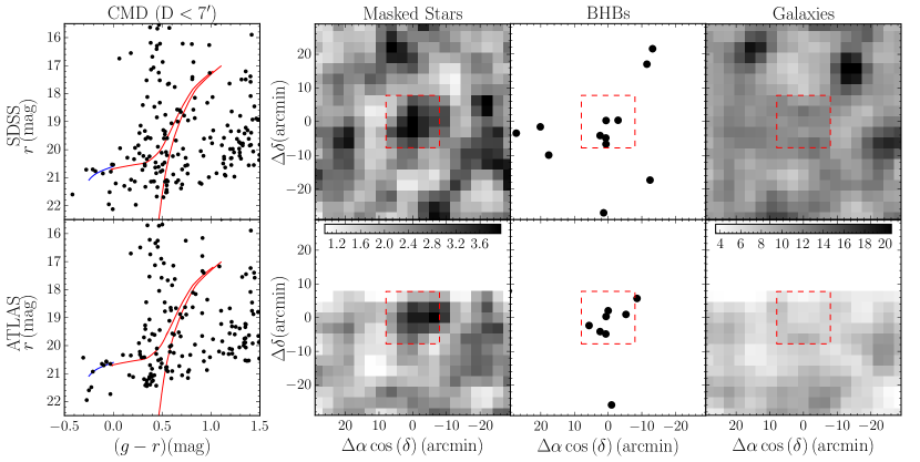
Figure 1: Aqu 2 as seen by ATLAS and SDSS. The panels on the top shows data from SDSS DR9, and the panels in the bottom show data from ATLAS. The leftmost panels show the CMD of the stars within 7′ of the center of Aqu 2. The red line shows a PARSEC isochrone with [Fe/H]=-1.8, age $12$ Gyr and m$-$M=20.16, and the blue line shows the outline of the blue horizontal branch from Deason, Belokurov & Evans (2011). In both SDSS and ATLAS CMDs there is an obvious overpopulation of BHB stars, but only in ATLAS are there hints of an RGB. In the middle left panel we show a density map (in units of objects per pixel) of stars inside the isochrone mask shown in Figure 3, and in the middle right panel we show the BHBs present in the field. In both tracers there is a visible overdensity. Finally, the rightmost panel shows the density map of galaxies, demonstrating that there is no obvious overdensity of galaxies at the location of Aqu 2.

2.2 Discovery

We discovered Aqu 2 by sifting through the ATLAS data armed with a version of the stellar overdensity detection algorithm (see e.g. Irwin, 1994; Koposov et al., 2008; Walsh, Willman & Jerjen, 2009; Koposov et al., 2015a; Torrealba et al., 2016). Briefly, the algorithm starts by filtering stars using an isochrone mask at a given age, metallicity and distance. The local density of stars is then measured and compared to the density at larger scales, i.e. the Galactic background/foreground. In practice, this is done by convolving the masked stellar number count distribution with a “Mexican hat” kernel: a difference between a narrow inner kernel (for the local density estimation) and a wide outer kernel (to gauge the background density). In our implementation, both kernels are two-dimensional Gaussians and the significance of the detection at each pixel is calculated by comparing the result of the convolution with the expected variance.

In the current implementation, we run the algorithm with two sets of isochrone masks: one that selects both MS and RGB stars, and a second one to pick out the likely BHB stars. The first mask is based on the most recent PARSEC evolutionary models (Bressan et al., 2012), from which, for simplicity, only old (12 Gyr) and metal poor ($[$Fe/H$]=-2$) population is chosen. The second mask is constructed from the BHB absolute magnitude ridgeline as a function of the $g-r$ color from Deason, Belokurov & Evans (2011). In both cases the masks widths are defined by the observed photometric errors above the minimum width of 0.1 magnitudes, in the case of PARSEC isochrones, and 0.2 magnitudes in the case of the BHBs (see Figure 3).

We applied the above search method to the ATLAS data using a grid of inner kernel sizes (from 1′ to 10′), and a grid of distance moduli ($15<m-M<23$) for both masks. The outer kernel size was fixed to 60′. As a result, two candidate lists were created, one for MS/RGB stars and one for BHBs. These were then cross-matched to create a single list of objects that were identified using both sets of tracers. In this combined list, Aqu 2 stood out as the only object of unknown nature, detected with a significance of $5.6\sigma$ in MS/RGB, and $4.9\sigma$ in BHBs. Aqu 2 also happens to be located within the footprint of the SDSS DR9, although it only had a significance of $4\sigma$ in MS/RGB stars, but a $5.5\sigma$ detection in BHBs. Figure 1 shows Aqu 2 as detected in both SDSS (top row) and ATLAS (bottom row). Overall, there is a strong evidence for a promising satellite candidate: in ATLAS, the MS/RGB stellar density map shows a clear overdensity (second panel, bottom row), which is not matched by any obvious galaxy clumping (fourth panel, bottom row). In the color-magnitude diagram (CMD, left panel) a hint of an RGB at $m-M\sim 20.16$ can be discerned between $19<r<22$. These are complemented by a handful of BHBs at a similar distance, which cluster tightly around the satellite location (third panel). Traces of a stellar overdensity can also be seen in the SDSS DR9 data (top row). While the SDSS RGB is not as prominent, the BHBs are readily identifiable, in perfect agreement with the significance values reported by the systematic search.

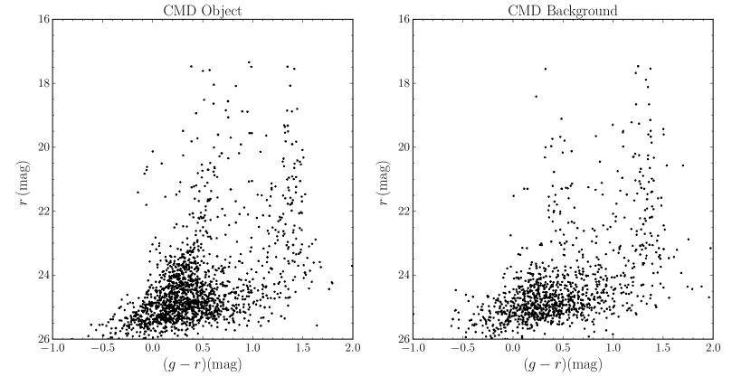
Figure 2: Color-magnitude diagram of Aqu 2 based the IMACS follow-up imaging. The left panel shows stars inside the half-light radius $r_{h}$, while the right panel shows stars from an equal area outside 7′ from the center. The CMD of the central areas of Aqu 2 demonstrates very clear evidence of the main sequence turn-off at r $\sim$ 24, the red giant branch and the horizontal branch at r $\sim$ 21. These features are all consistent with the stellar population at a distance modulus of m$-$M$\sim 20.16$ ($\sim 108$ kpc) and match well with the features visible in the VST and SDSS data.

3 Photometric follow-up

3.1 IMACS imaging

To confirm the nature of the candidate overdensity described above, deeper photometric data was obtained using the 6.5 m Walter Baade telescope at the Las Campanas observatory in Chile. The images were taken on 19 Aug 2015 using the f/4 mode of the Inamori-Magellan Areal Camera & Spectrograph (IMACS) which provides a 15.4$\arcmin\times$15.4$\arcmin$ field of view with a mosaic of 8 2k$\times$4k CCDs (Dressler et al., 2011). We employed 2x2 binning which gives a pixel scale of $\sim$ 0.22$\arcsec$/pixel. A total of 4 exposures centered on Aqu 2 were taken in each of the $g$ and $r$ filters giving a total exposure time of 19 minutes in $g$ and 23.5 minutes in $r$. After standard reduction steps, the images were astrometrically calibrated using astrometry.net software (Lang et al., 2010) and stacked using the SWARP software (Bertin et al., 2002).

3.2 Catalog Generation

The IMACS object catalogs were created by performing photometry on the images using SExtractor/PSFex (Bertin & Arnouts, 1996) as described in Koposov et al. (2015a). First, an initial SExtractor pass was done to create the source list required by PSFex. Then, PSFex is run to extract the point spread function (PSF) shape, which is then used in the final SExtractor pass. This procedure delivers estimates of the model and the PSF magnitudes for each object, as well as estimates of the SPREAD_MODEL and SPREADERR_MODEL parameters. The final catalog is assembled by merging the g and r bands within a cross-match distance of 0.7$\arcsec$, only selecting objects with measurements in both bands. We calibrated the instrumental magnitudes by cross-matching the catalog with the SDSS. The resulting zero-point is measured with a photometric precision of $\sim 0.1$ mag in both bands. Finally, likely stars are separated from likely galaxies by selecting all objects with $|\texttt{SPREAD\_MODEL}|<0.005+\texttt{SPREADERR\_MODEL}$ (see e.g. Desai et al., 2012; Koposov et al., 2015a).

Figure 2 shows the CMD of the area around Aqu 2 constructed using the merged stellar catalogs from the IMACS data. Only stars within the half light radius of Aqu 2 (see Section 3.3 for details on its measurement) are displayed in the left panel, while the stars of an equal area outside the central region are given in the right panel for comparison. The left panel of the Figure leaves very little doubt as to the nature of the candidate: the familiar CMD features of a co-eval and co-distant old stellar population, a very prominent MS turn-off, the strong RGB and a clumpy BHB are all conspicuous. Note that while the CMD shown in the right panel contains mostly Galactic foreground, there are hints of the RGB and MSTO of Aqu 2 here too, which is consistent with the object extending beyond its half light radius (see Section 3.3 for further discussion). Figure 3 shows the same CMD as in the left panel of Figure 2 but with various stellar sub-populations highlighted. To guide the eye, the PARSEC isochrone with [Fe/H]=$-1.8$, age of 12 Gyr, and offset to $m-M=20.16$ is over-plotted in red. This isochrone is used to create the CMD mask to select stars belonging to the satellite. Thus, the age and the metallicity of the isochrone were chosen to maximize the number of member stars within the mask. Orange, red, and blue filled circles mark stars identified as foreground, Aqu 2 RGB and Aqu 2 BHB stars respectively based on follow-up spectroscopy (see Section 4 for details). The red dashed line shows the isochrone mask used to select the likely MSTO and RGB members of the satellite, and the region in blue is the area where probable BHB member stars lie. The shape and the position of the blue area is based on the BHB ridge- line given in Deason, Belokurov & Evans (2011). These likely BHB member stars are also used to measure the distance modulus of Aqu 2 as $m-M=20.16\pm 0.07$, which corresponds to a heliocentric distance of $108\pm 3$ kpc.

3.3 Structural Parameters

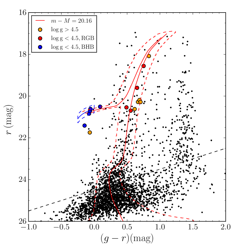
Figure 3: Color magnitude diagram of the central 7′ of Aqu 2. The red line is a PARSEC isochrone with [Fe/H]=-1.8, age $12$ Gyr and m$-$M=20.16. The blue dashed contour marks the selection area of BHB stars (with 5 stars) used to constrain the distance to Aqu 2 and the dashed red line delineates the isochrone mask. The dashed black line corresponds to $g=24.5$, which is the limiting magnitude that we use when determining structural parameters of Aqu 2. Large filled circles mark stars with measured spectra, in orange we show likely dwarf stars with $\log({\rm{g})}>4$ (representing contamination), and in blue and red we show giants with $\log({\rm{g})}<4$ (likely BHB and RGB stars respectively).

The structural parameters of Aqu 2 are determined by modelling the distribution of the likely member stars based on their colors and magnitudes (i.e. those located inside the isochrone mask outlined with the red dashed line in Figure 3) in the IMACS field of view (see e.g., Martin, de Jong & Rix, 2008; Koposov et al., 2015a; Torrealba et al., 2016, for a similar approach). To reduce the contamination from galaxies misclassified as stars, we only use stars brighter than $g=24.5$. The spatial model for the stellar distribution consists of a flat Galactic background/foreground density and a 2-dimensional elliptical Plummer profile (Plummer, 1911). The Plummer profile is defined as:

$$P_{obj}(x,y|\Theta)=\frac{1}{\pi a^{2}\left(1-e\right)}\left(1+\frac{\tilde{r}^{2}}{a^{2}}\right)^{-2},$$ (1)

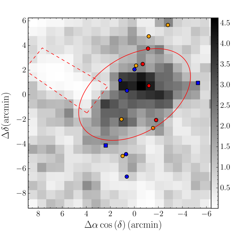
Figure 4: Density maps of stars within the isochrone mask from the follow-up imaging. The red solid line shows the elliptical half-light contour of the best fit model, and the red dashed line marks a region with the bright star that was excised from the analysis. The orange, red and blue circles mark the locations of stars spectroscopically confirmed as foreground, RGB and BHB stars respectively. Blue squares show BHB stars photometrically selected using the blue box of Figure 3, but without measured spectra.

where $x$ and $y$ are the on-sky coordinates which have been projected to the plane tangential to the center of the object, $\Theta$ is a shorthand for all model parameters, namely, the elliptical radius $a$, the coordinates of the center $x_{0}$, $y_{0}$, the positional angle of the major axis $\theta$, and the ellipticity of the object $e$:

$$\tilde{r} = \sqrt{\tilde{x}^{2}+\tilde{y}^{2}}$$ (2)

$$\tilde{x} = (\left(x-x_{0}\right)\,\cos\theta-\left(y-y_{0}\right)\sin\theta)/\left(1-e\right)$$

$$\tilde{y} = \left(x-x_{0}\right)\sin\theta+\left(y-y_{0}\right)\cos\theta.$$

The probability of observing a star at $x,y$ is then:

$$P(x,y|\Theta)=\frac{f}{A_{obj}(\Theta)}\,P_{obj}(x,y|\Theta)+(1-f)\,\frac{1}{A},$$ (3)

with $A$ being the area of the data footprint, $f$ is the fraction of stars belonging to the object rather than foreground and $A_{obj}(\Theta)$ is the integral of the Plummer model from Eq. 1 over the data footprint.

With Eq. 3 defining the distribution for positions of stars, we sample the posterior distribution of parameters of the model $P(\Theta|D)$ using MCMC. We use the affine invariant ensemble sampler (Goodman & Weare, 2010) implemented as an emcee Python module by Foreman-Mackey et al. (2013) with flat priors on all the model parameters except $a$, in which we use the Jeffreys prior $P(a)\propto\frac{1}{a}$. The best-fit parameters were determined from the mode of the marginalized 1D posterior distributions, with error-bars determined from the 16% 84% percentiles of the posterior distribution. The best-fit model returns a marginally elliptical Plummer profile with $e=0.4\pm 0.1$ and an elliptical half-light radius of $r_{h}=5\arcmin.1\pm 0\arcmin.8$ corresponding to a physical size of $\sim$ 160 pc.

The density map of isochrone selected stars is shown in Figure 4. The dark elliptical blob in the center of the image is Aqu 2. The red solid line gives the half-light contour of the best-fit model while the red dashed line marks the region affected by a bright star, that was masked out. Orange, red and blue filled circles give the positions of the handful of stars with measured spectra as described above. Figure 5 presents the 1D radial profile of Aqu 2 together with the best-fit model (red line), which clearly provides an adequate fit to the data in hand.

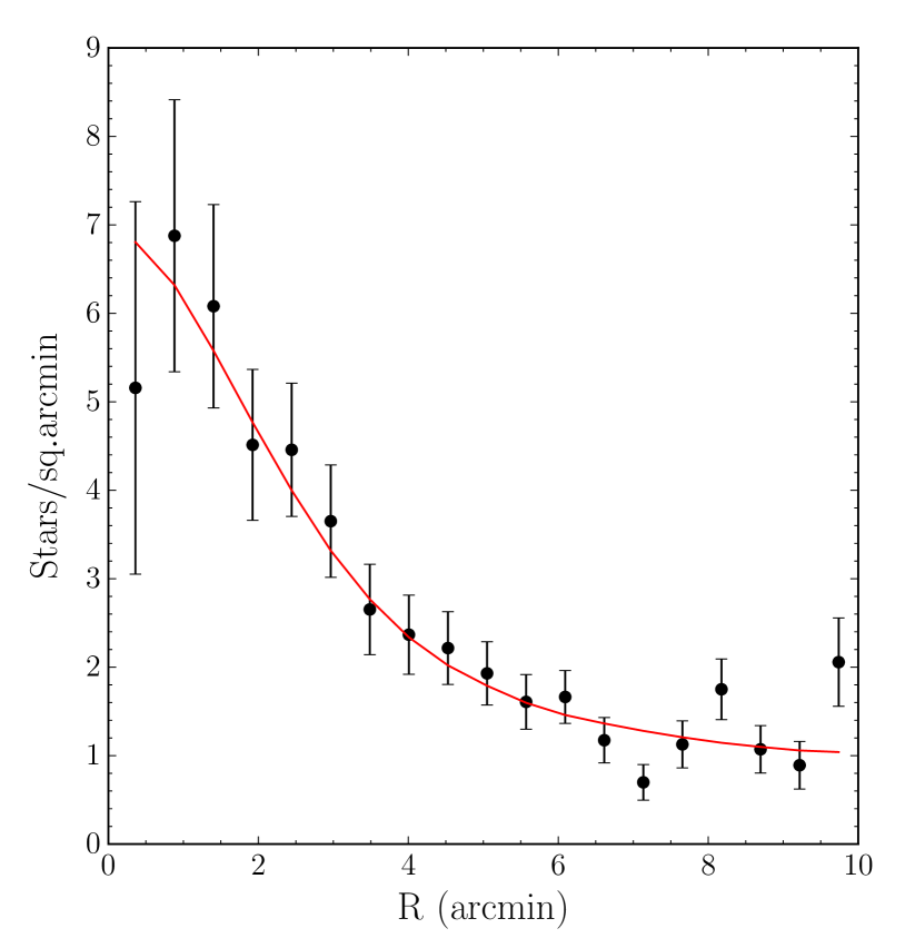
Figure 5: Radial number density profile of Aqu 2 as probed by the stars inside the isochrone mask shown in Figure 2. The red line shows the best fit model, which is formed by a flat background and a elliptical Plummer profile with $r_{h}=5\arcmin.1$ and $1-\rm{b/a}=0.39$

We estimate absolute luminosity of Aqu 2 by first counting the number of observed Aqu 2 members. We do this by measuring the fraction of member stars, $f$, in Eq. 3 using a broad isochrone mask (with a limiting width of 0.2 magnitudes), and with all the parameters of the model but $f$, fixed. For this calculation we use a limiting magnitude of $\sim$24.5 in both $g$ and $r$ bands, as above this limit the point source completeness of our catalog is higher than 90%. The fraction $f$ of the total number of stars belonging to Aqu 2 that are brighter than 24.5 in both $g$ and $r$ is measured to be $0.50\pm 0.04$, which translates into $282\pm 24$ stars. Subsequently, we can now compute the absolute magnitude of Aqu 2 by assuming a single stellar population following a PARSEC isochrone with Chabrier initial mass function (Chabrier, 2003). Using the Parsec isochrone with metallicity of $-1.8$ with an age of 12 Gyr yields an estimation of the absolute luminosity of $M_{V}=-4.27\pm 0.1$ without including BHBs. Note that the contribution from BHBs is added separately, owing to the uncertainties in the modeling of HB morphologies (see e.g. Gratton et al., 2010). Assuming that Aqu 2 contains $\sim$ 7 BHB stars, we derive their contribution to the luminosity of the object $M_{V}(BHB)=-1.62\pm 0.09$. Combined contribution from stars within the isochrone mask and the BHBs added together gives the final luminosity for Aqu 2 of $M_{V}=-4.36\pm 0.14$. We note that while the metallicity of the isochrone used for calculating the luminosity of the object is higher than the metallicity that we derived spectroscopically $[Fe/H]=-2.3\pm 0.5$ (see Section 4 for details), we have verified that our estimate of the Aqu 2 luminosity is not sensitive to changes of metallicity within 0.2 dex.

4 Spectroscopic follow-up

Aqu 2 was observed on the night of 11th September 2015, using the DEep Imaging Multi-Object Spectrograph (DEIMOS) on the 10 m Keck II telescope. DEIMOS is a slit-based spectrograph, and one mask centered on Aqu 2 was produced using the DEIMOS mask design software, DSIMULATOR, with VST ATLAS photometry described above. Stars were prioritized for observation based on their position in the CMD of Aqu 2, and proximity to the photometric centre of the object. Only stars with $i-$band magnitude $<22$ were selected for observation, to ensure that our final spectra had sufficient $S/N$ to determine a velocity ($S/N>3$ per pixel). Out 20 potential member stars observed, 15 were successfully reduced. These 15 stars are identified as large filled circles on Figures 3 and 4. The Aqu 2 mask was observed with a central wavelength of 7800Å, using the medium resolution 1200 line/mm grating ($R\sim 1.4$ Å at our central wavelength), and the OG550 filter. This gave a spectral coverage of $\sim 5600-9800$ Å, isolating the region of the calcium II triplet (Ca II) at $\lambda\sim 8500$ Å. The target was observed for 1 hour, split into $3\times 20$ minute integrations. The conditions were ideal, with seeing ranging from $0.4-0.5^{\prime\prime}$.

We reduced the spectra using our standard DEIMOS pipeline, described in Ibata et al. (2011) and Collins et al. (2013). Briefly, the pipeline identifies and removes cosmic rays, corrects for scattered light, performs flat-fielding to correct for pixel-to-pixel variations, corrects for illumination, slit function and fringing, wavelength calibrates each pixel using arc-lamp exposures, performs a two-dimensional sky subtraction, and finally extracts each spectrum without resampling in a small spatial region around the target.

4.1 Spectral modelling

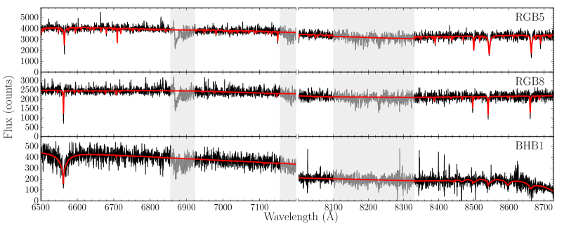
Figure 6: Example of the observed spectra (black) together with our best fit model (red) for a field star (top), an RGB star (middle), and a BHB star (bottom). The grey-shaded regions mark regions affected by telluric absorption that were masked out during model fitting of the spectra.

The spectroscopic properties of the stars observed were inferred using a procedure similar to that described in Koposov et al. (2011, 2015b), i.e., via direct pixel-fitting of a suite of template spectra to the observed spectrum. The template spectra were drawn from the medium resolution PHOENIX library (Husser et al., 2013). The library spectra are given at a resolution of $R=10000$ in a wavelength range between $3000$ Å and $25000$ Å and cover a wide range of stellar parameters: $2300$ K$\leq\rm{T}_{\rm{eff}}\leq 12000$ K; $0\leq\log{\rm{g}}\leq 6$; $-4\leq[$Fe/H$]\leq 1$; and $-0.2\leq[\alpha$/Fe$]\leq 1.2$. In practice, we pick values in a model grid using a 100 K step size for $\rm{T}_{\rm{eff}}<7000$ and 200 K for $\rm{T}_{\rm{eff}}>7000$, 0.5 dex in $\log{\rm{g}}$, 0.5 dex for $[$Fe/H$]>-2$ and 1 dex for $[$Fe/H$]<-2$, and two discrete values for $[\alpha$/Fe$]=\{0,0.4\}$. All template spectra are degraded from the initial resolution to the observed resolution of R=$5900$.

Following Koposov et al. (2011, 2015b), in order to account for the absence of flux calibration of the spectra the models are represented as template spectra multiplied by a polynomial of wavelength of degree $N$ defined as:

$$P(\lambda)=\sum\limits_{j=0}^{N}a_{j}\lambda^{j},$$ (4)

where $a_{j}$ are the polynomial coefficients. Thus, the final model spectrum is as follows:

$$M(\lambda,i,V)=P(\lambda)T_{i}\left(\lambda\left(1+\frac{V}{c}\right)\right),$$ (5)

where $T_{i}$ is the downsampled $i$-th template.

The log-likelihood of each model is then defined as $-0.5\chi^{2}$, where $\chi^{2}$ is calculated summing the squared standardized residuals between the data and the model over all pixels in the spectrum:

$$\chi^{2}(i,V)=\sum\limits_{k}\left(\frac{O(\lambda_{k})-M(\lambda_{k},i,V)}{E(\lambda_{k})}\right)^{2},$$ (6)

where $O(\lambda_{k})$ is the observed spectra, $E(\lambda_{k})$ the uncertainties, and $\lambda_{k}$ the wavelength at each pixel. Examples of the three observed spectra, a field star, and an RGB and a BHB, both members of Aqu 2, with their corresponding best-fit models are shown in Figure 6.

For each star, the best-fit spectral model is obtained in two steps. First, we test velocities between -700 km s^-1 and 700 km s^-1 with a resolution of 5 km s^-1 - while simultaneously varying other model parameters - to zoom-in onto the approximate heliocentric velocity solution. Next, we refine the velocity grid resolution to 0.5 km s^-1 in the region around the best-fit velocity obtained in the first pass. The final velocity and the stellar atmosphere parameters ($T_{\rm{eff}},\log{\rm{g}},[$Fe/H$]$ and $[\alpha$/Fe$]$) are found by marginalizing the likelihood over the nuisance parameters. We choose to use flat priors on all parameters apart from temperature, for which we use Gaussian priors based on the $g-r$ colour of the star. The temperature prior is dictated by the colour-temperature relation obtained for the VST-ATLAS stars with spectroscopic effective temperatures measured by the SEGUE Stellar Parameter Pipeline (Lee et al., 2008a, b; Allende Prieto et al., 2008). Finally, the preferred values for the model parameters, and their associated uncertainties, are measured from 1-D marginalized posterior probability distributions, corresponding to the $16\%,50\%$ and $84\%$ percentiles. These are reported in Table 2.

Table 2: Stellar parameters of spectroscopic targets

Object	$\alpha$(J2000)	$\delta$(J2000)	g	r	$V_{h}$	$T_{\rm eff}$	$\log{\rm g}$	$[$Fe/H$]$	$\chi^{2}$/dof	Member?
	(deg)	(deg)	(mag)	(mag)	(km/s)	(K)	(dex)	(dex)
RGB1	$338.45496$	$-9.37256$	$21.24$	$20.62$	$-115.9\pm 1.2$	$4896_{-31}^{+347}$	$-$	$-1.5_{-0.0}^{+0.4}$	2.21	N
RGB2	$338.45067$	$-9.36172$	$21.03$	$20.54$	$-78.7\pm 2.0$	$5090_{-21}^{+46}$	$3.3_{-0.4}^{+0.3}$	$-3.0_{-0.1}^{+0.0}$	2.16	Y
RGB3	$338.46083$	$-9.31522$	$20.26$	$19.6$	$-75.1\pm 1.0$	$5093_{-10}^{+5}$	$2.4_{-0.1}^{+0.1}$	$-2.0_{-0.0}^{+0.0}$	4.57	Y
RGB4	$338.49946$	$-9.36058$	$20.95$	$20.28$	$-131.4\pm 1.5$	$5233_{-136}^{+246}$	$4.6_{-0.4}^{+0.7}$	$-2.0_{-0.0}^{+0.4}$	2.3	N
RGB5	$338.47883$	$-9.28794$	$18.91$	$18.08$	$43.5\pm 0.3$	$5098_{-3}^{+1}$	$5.0_{-0.0}^{+0.0}$	$-0.5_{-0.0}^{+0.0}$	9.62	N
RGB6	$338.46208$	$-9.26497$	$21.25$	$20.7$	$-77.7\pm 3.6$	$4970_{-127}^{+257}$	$3.1_{-0.9}^{+0.9}$	$-2.1_{-0.3}^{+0.1}$	1.85	Y
RGB7	$338.46104$	$-9.24833$	$20.88$	$20.19$	$-247.4\pm 2.6$	$5095_{-9}^{+4}$	$5.8_{-0.3}^{+0.2}$	$-1.0_{-0.1}^{+0.0}$	2.51	N
RGB8	$338.46954$	$-9.28583$	$19.31$	$18.56$	$-63.3\pm 0.4$	$4898_{-2}^{+1}$	$0.5_{-0.1}^{+0.0}$	$-2.0_{-0.0}^{+0.0}$	8.43	Y
RGB9	$338.43417$	$-9.23303$	$20.99$	$20.28$	$-212.3\pm 3.1$	$5219_{-147}^{+161}$	$4.8_{-0.7}^{+0.5}$	$-1.0_{-0.2}^{+0.4}$	2.33	N
BHB1	$338.49192$	$-9.43825$	$20.76$	$20.84$	$-70.6\pm 4.1$	$7825_{-127}^{+132}$	$3.8_{-0.2}^{+0.2}$	$-0.9_{-0.2}^{+0.3}$	1.74	Y
BHB2	$338.49288$	$-9.40789$	$20.65$	$20.71$	$-65.2\pm 3.6$	$7780_{-54}^{+97}$	$3.5_{-0.1}^{+0.0}$	$-1.5_{-0.3}^{+0.4}$	1.86	Y
BHB3	$338.49775$	$-9.41033$	$21.68$	$21.74$	$201.9\pm 11.9$	$8407_{-192}^{+193}$	$5.8_{-0.3}^{+0.2}$	$-0.2_{-0.4}^{+0.4}$	1.9	N
BHB4	$338.49167$	$-9.32186$	$20.6$	$20.51$	$-62.6\pm 4.4$	$7578_{-38}^{+17}$	$3.5_{-0.1}^{+0.0}$	$-1.9_{-0.3}^{+0.3}$	1.98	Y
BHB5	$338.48112$	$-9.29314$	$20.56$	$20.62$	$-71.5\pm 4.5$	$7788_{-144}^{+164}$	$3.2_{-0.2}^{+0.2}$	$-0.6_{-0.3}^{+0.1}$	1.92	Y
BHB6	$338.50117$	$-9.308$	$21.27$	$21.41$	$-94.9\pm 16.9$	$8216_{-227}^{+191}$	$3.9_{-0.1}^{+0.1}$	$-3.1_{-0.9}^{+1.1}$	1.55	Y

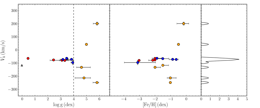
Figure 7: Heliocentric radial velocity plotted against $\log{\rm{g}}$ (left) and $[$Fe/H$]$ (middle) for 15 stars with observed spectra. Stars in orange have $\log{\rm{g}}>4$, and are likely field contamination. The gray dot is the star without a good $\log{\rm{g}}$ measurement. Rightmost panel shows the generalized histogram for the radial velocity with a Epanechnikov kernel with 10 km s^-1 bandwidth. The velocity distribution of likely members has a very well defined peak at -71 km s^-1

Figure 7 displays the distribution of heliocentric velocities as a function of surface gravity $\log{\rm{g}}$ (left panel) and metallicity $[$Fe/H$]$ (middle panel) for all stars in the spectroscopic dataset. We conjecture that stars with $\log{\rm{g}}>4$ are likely foreground contaminants, i.e. nearby MS stars. This hypothesis is supported by a large spread in velocity observed for this subgroup. In contrast, the velocity distribution of 9 stars (4 RGBs and 5 BHBs) with $\log{\rm{g}}<4$ has a well-defined narrow peak at V_h$\sim$ -71 km s^-1. This confirms that Aqu-2 is indeed a bona-fide Milky Way satellite. It is also important that all the BHB candidate stars have velocities consistent with the peak. We measure the systemic velocity $V_{h}$ and the velocity dispersion $\sigma_{V}$ of Aqu 2, by modelling the velocity distribution of likely star members, i.e. the stars with $\log{\rm{g}}<4$ as a single Gaussian with mean $V_{h}$ and dispersion $\sigma_{v}$. We sample the likelihood of the model using emcee assuming flat priors for the mean and the Jeffreys priors for the dispersion. The satellite mean velocity is thus determined to be $V_{h}=-71.1\pm 2.5$ km s^-1, corresponding to $V_{\rm GSR}=49$ km s^-1 assuming the Local Standard of Rest of 235 km s^-1 and the Solar peculiar motion as measured by Schönrich, Binney & Dehnen (2010). Aqu 2’s velocity dispersion is $\sigma_{V}=5.4^{+3.4}_{-0.9}$ km s^-1. Figure 8 shows the corresponding posterior distributions.

We can also estimate the mean metallicity of Aqu 2 by using the 4 RGB member stars: $[$Fe/H$]=-2.3\pm 0.5$. Notice a quite large error-bar that is expected given the small number of stars, low resolution of the spectra and step-size of 0.5 dex in the template grid used. However, most importantly, the spectroscopic metallicity measured is consistent on the 1 $\sigma$ level with the metallicity of the isochrone used in our photometric analysis.

According to the results of the previous Section, the extended size of Aqu 2 suggests that it should be classified as a dwarf galaxy, as currently, there are no known star clusters that large. We further firm up this classification by calculating the dynamical mass. Using the estimator of Walker et al. (2009), we calculate the mass enclosed within the half-light radius to be $2.7^{+6.6}_{-0.5}\times 10^{6}M_{\odot}$ which corresponds to a mass-to-light ratio of $1330^{+3242}_{-227}$. This is the second overwhelming piece of evidence that Aqu 2 is indeed a typical dark matter dominated UFD. The following cautionary notes are worth bearing in mind. First, while the current data allow us to resolve the velocity dispersion of Aqu 2, the value is inferred, using only a small number of tracers. Furthermore, the mass estimate may be affected by the strong elongation of the dwarf, which can be both a sign of an aspherical matter distribution as well as out-of-equilibrium state of its member stars.

5 Discussion and Conclusions

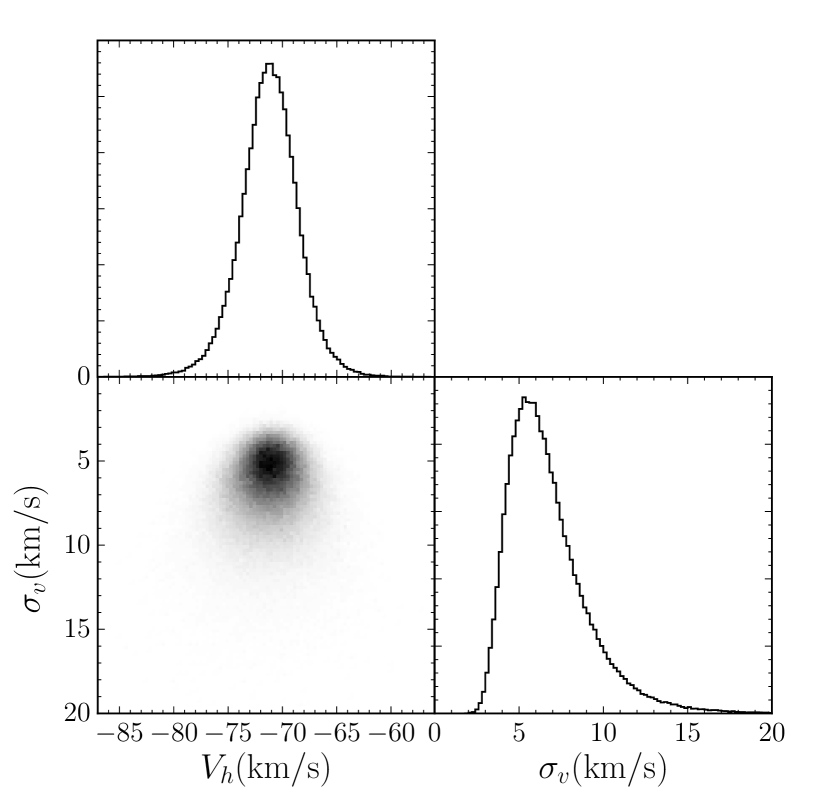
Figure 8: Posterior distribution for the heliocentric velocity and velocity dispersion of Aqu 2. These are found by modelling the observed velocity distribution by a single Gaussian. Both posterior distributions shows a well defined maxima, with $\sigma_{V}$ having a long tail towards larger dispersions.

Figure 9 shows the distribution of the Milky Way dwarf satellites in the plane of absolute magnitude $M_{V}$ and heliocentric distance $D_{\odot}$. Objects are coloured according to the imaging survey they were discovered in. The so-called Classical dwarfs (orange) appear to be detectable at any distance throughout the virial volume of the Galaxy, independent of their absolute magnitude. This is unsurprising given their high intrinsic luminosities. However, the UFDs, nominally identified as dwarfs with $M_{V}>-8$ show a strong selection bias as a function of heliocentric distance. According to Koposov et al. (2008), the detectability of a satellite as traced by its stellar members, depends primarily on its surface brightness and heliocentric distance. So far, most of the dwarfs discovered are brighter than $\sim 30-31$ mag arcsec^-2 as illustrated in Figure 10. Curiously, all satellites with $r_{h}<100$ pc, lie above the $\mu=30$ mag arcsec^-2 line. However, the larger objects seem to obey a slightly fainter detection limit, namely $\mu=31$ mag arcsec^-2. To help analyze the distribution of the satellites in the 3D space spanned by their luminosity, surface brightness and distance, the symbol size in Figure 9 represents the effective surface brightness of objects, with bigger circles corresponding to smaller (i.e. brighter) values of $\mu$.

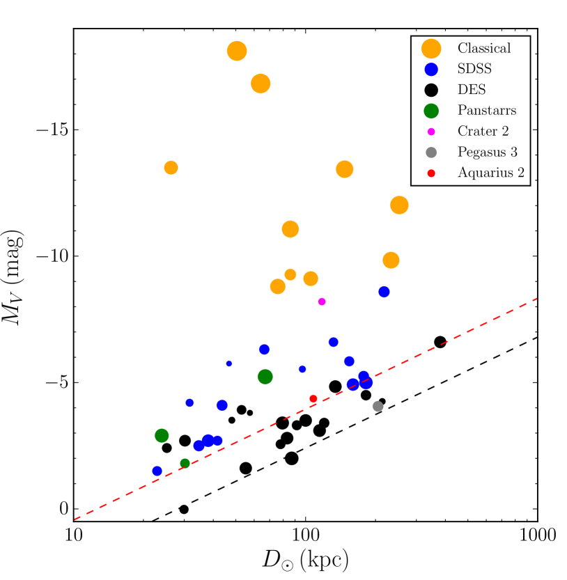
Figure 9: Absolute magnitude versus heliocentric distance for dwarf galaxies within 400 kpc. The size of the markers reflects the surface brightness of the dwarfs, with the largest points showing the brightest galaxies. We show classical dwarfs in orange, dwarfs discovered in SDSS in blue, dwarfs discovered in DES in black, and dwarfs discovered in PanStarss in green. The red/magenta/gray points shows the position of Aqu 2/Crater 2/Pegasus 3. The red dashed line shows the detectability limit for SDSS as determined by (Koposov et al., 2008) and the black dashed line the approximate limit for DES (Jethwa, Erkal & Belokurov, 2016).

As discussed in Koposov et al. (2008), the distance of a satellite plays an important role in determining whether it is going to be detected or not. At a given heliocentric distance, of all objects below the nominal surface brightness limit (as discussed above), only those brighter than a certain limiting absolute magnitude can be securely identified. Koposov et al. (2008) provide an expression for the limiting absolute magnitude as a function of distance. This model is shown as a dashed red line in Figure 9. Indeed, all SDSS-based detections appear to lie above this detection boundary. Also shown (dashed black line) is a version of the detectability limit derived by Jethwa, Erkal & Belokurov (2016) for the objects identified in the DES data. Amongst the SDSS objects, together with Leo IV, Leo V and Her, Aqu 2 forms a group that sits nearest to the nominal luminosity boundary. Moreover, it is also one of the lowest surface brightness satellites beyond 100 kpc from the Sun. Thus, Aqu 2 is the only dwarf galaxy detected at both the luminosity and the surface brightness limits. This is probably the reason why this object had not been identified before.

The key reason for the surface brightness detection limit for Milky Way satellites as measured by Koposov et al. (2008) is the balance between the foreground density of stellar contaminants, the background density of misclassified compact galaxies and the number of satellite member stars. However, when BHB stars are used for satellite detection, they represent a completely different regime, as the surface density of contaminating foreground A-type stars and background compact galaxies are orders of magnitude lower compared to using MSTO or RGB-colored stars. Furthermore, for the horizontal branch to be populated, the luminosity of the satellite needs to be more than a certain critical value. Thus, it would not be surprising if the actual combined BHB+RGB detection boundary deviated somewhat from the simple limiting surface brightness prescription of Koposov et al. (2008).

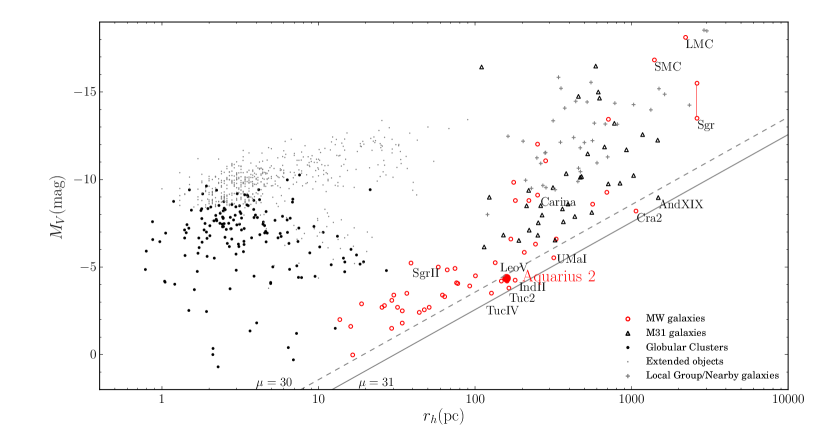
Figure 10: Absolute magnitude versus half-light radius. Local galaxies from McConnachie (2012) (updated September 2015) are shown with different symbols. Dwarf galaxy satellites of the Milky Way are shown with red open circles, the M31 dwarfs with black unfilled triangles, and other nearby galaxies with gray crosses. Note that for the Sgr dwarf, we also give the estimate of the progenitor’s original luminosity from Niederste-Ostholt et al. (2010). Black dots are the Milky Way globular clusters measurements from (Harris, 2010; Belokurov et al., 2010; Muñoz et al., 2012; Balbinot et al., 2013; Kim & Jerjen, 2015a; Kim et al., 2015c, b; Laevens et al., 2015; Weisz et al., 2015) and gray dots are extended objects smaller than 100 pc from (Brodie et al., 2011). The black solid (dashed) line corresponds to the constant level surface brightness within half-light radius of $\mu=31$ (30) $\rm{mag}\,\rm{arcsec}^{-2}$, which is approximately the surface brightness limit of the searches for resolved stellar systems in the SDSS (Koposov et al., 2008). The position of the recently discovered Crater 2 (Torrealba et al., 2016) is also shown.

Moreover, Figure 10 hints at an intriguing possibility that the intrinsic distribution of the Milky Way satellites forms a reasonably tight sequence in luminosity-size space along the line connecting the LMC and the newly discovered Aqu 2. The one object that clearly appears to lie off this sequence is the Sgr dwarf, which is known to have lost most of its stars (see e.g. Niederste-Ostholt et al., 2010), entering the last throws of the tidal disruption. Objects like UMa I, Leo V, Ind II would then represent the more frequent occupants of this dwarf-galaxy main sequence, while currently observed objects with smaller sizes ($r_{h}<100$ pc) may either represent a sub-population of tidally disrupting objects, or those with properties transitional between globular clusters and dwarf galaxies.

5.1 The LMC connection?

As illustrated in Figure 9, between $\sim$60 and $\sim$130 kpc, there appears to be a paucity of SDSS UFDs detected, with only one such object known, namely Bootes I. Aqu 2, at $\sim$110 kpc, helps to fill in this gap, but is almost $\sim$2 magnitudes fainter. Of course, there are plenty even fainter dwarf satellites in this heliocentric distance range, i.e. those discovered in the DES data. However, these cluster spatially around the LMC and the SMC, and, as shown by Jethwa, Erkal & Belokurov (2016), are likely to be associated with the accretion of the Clouds by the Galaxy.

Aqu 2 lies just 9 kpc from the current orbital plane of the LMC, as defined by the most recent measurement of the LMC 3D velocity vector Kallivayalil et al. (2013). We now consider whether this is a chance alignment, or signals some association between these Galactic satellites. This question is further motivated by the recent discovery of 17 dwarf galaxies and dwarf galaxy candidates discovered in data taken from the Dark Energy Survey (DES Koposov et al., 2015a; Bechtol et al., 2015; Kim & Jerjen, 2015b; Drlica-Wagner et al., 2015) many of which have been shown to be likely associated with the Magellanic Clouds (Yozin & Bekki, 2015; Deason et al., 2015; Jethwa, Erkal & Belokurov, 2016), thus confirming a generic prediction of cold dark matter cosmological models whereby the hierarchical build up of structure leads to groupings of dwarf satellite galaxies in the Galactic halo. Most recently, Jethwa, Erkal & Belokurov (2016) investigated this by building a dynamical model of satellites of the Magellanic Clouds. This included the gravitational force of the Milky Way, LMC and the SMC, the effect of dynamical friction on the orbital history of the Magellanic Clouds, and marginalized over uncertainties in their kinematics. Fitted against DES data, their results suggested that the LMC may have contributed $\sim 70$ dwarfs to the inventory of satellite galaxies, i.e. $\sim$30% of the total population.

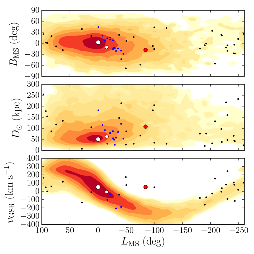
Figure 11: Comparison of the phase space distribution of known dwarf galaxies within 300 kpc (plotted symbols) with a simulated distribution of LMC satellites (coloured contours). The top panel shows the on-sky distribution in Magellanic Stream co-ordinates $(L_{\mathrm{MS}},B_{\mathrm{MS}})$. The middle panel shows heliocentric distance, and the bottom panel line-of-sight velocity in the Galactic standard of rest, both as functions of $L_{\mathrm{MS}}$. Contour colours step in factors of two density, normalised independently per panel. The LMC and SMC are represented by the small and large white circles, other dwarf galaxies as dots (blue if discovered in DES, black otherwise) and Aqu 2 as the red symbol.

Figure 11 shows the distribution of LMC satellites from the maximum likelihood model of Jethwa, Erkal & Belokurov (2016) as coloured contours, with known dwarfs shown as plotted symbols. The top panel shows the on-sky distribution in Magellanic Stream co-ordinates $(L_{\mathrm{MS}},B_{\mathrm{MS}})$ (defined in Nidever, Majewski & Burton, 2008), where latitude $B_{\mathrm{MS}}=0$ traces the centre of the HI gas distribution, which is slightly offset from the LMC proper motion vector. We see that Aqu 2 (shown by the red symbol) lies at relatively small Magellanic latitude $B_{\mathrm{MS}}=-17.8$ deg, and - as shown in the middle panel - is well within the scope of the simulated distance distribution of Magellanic satellites. The bottom panel, however, shows that at its Magellanic longitude, Aqu 2 is moving too slowly to be a member of the trailing debris of LMC satellites. This is generically true over the grid of models presented by Jethwa, Erkal & Belokurov (2016) and hence we disfavour a Magellanic origin for Aqu 2, preferring instead a scenario where it is part of a virialised population of Milky Way satellites.

5.2 Summary

Aqu 2 was discovered at the very edge of the VST ATLAS footprint as an overdensity of RGB stars. What made it stand out amongst the several other candidates with similar significance is the presence of a prominent BHB. Moreover, the object also appeared in the list of significant overdensities produced using the SDSS DR9 data, located, equally, not very far from the edge of the footprint. To establish the nature of the candidate, we have obtained deep follow-up imaging of Aqu 2 with Baade’s IMACS camera, as well as spectroscopy with Keck’s DEIMOS, which fully confirmed that the object is a true Milky Way satellite. Given the satellite size of $\sim 160$ pc and the stellar velocity dispersion of $5.4^{+3.4}_{-0.9}$ km s^-1, Aqu 2 is undoubtedly a dwarf galaxy. The shape of Aqu 2 is mildly elliptical $1-b/a\sim 0.4$, and the radial velocity indicates that Aqu 2 is currently moving away from the Galacic center, on its way to apo-galacticon. Taken at face value, its structural and kinematic parameters imply an extremely high mass-to-light ration of $M/L=1330^{+3242}_{-227}$. We stress, however, that the determination of the structural parameters of Aqu 2, particularly the half-light radius, can be significanlty improved with wider field-of-view observations. Similarly, the velocity dispersion measurement would benefit from a larger sample of satellite member stars. The discovery of Aqu 2 is a testimony to the fact that many more faint dwarfs are surely still lurking in the SDSS and VST ATLAS datasets.

References

- Abazajian et al. (2009) Abazajian K. N. et al., 2009, ApJS, 182, 543
- Adelman-McCarthy et al. (2007) Adelman-McCarthy J. K. et al., 2007, ApJS, 172, 634
- Aihara et al. (2011) Aihara H. et al., 2011, ApJS, 193, 29
- Allende Prieto et al. (2008) Allende Prieto C. et al., 2008, AJ, 136, 2070
- Balbinot et al. (2013) Balbinot E. et al., 2013, ApJ, 767, 101
- Bechtol et al. (2015) Bechtol K. et al., 2015, ApJ, 807, 50
- Belokurov (2013) Belokurov V., 2013, NARev, 57, 100
- Belokurov et al. (2014) Belokurov V. et al., 2014, MNRAS, 437, 116
- Belokurov et al. (2010) Belokurov V. et al., 2010, ApJ, 712, L103
- Belokurov et al. (2009) Belokurov V. et al., 2009, MNRAS, 397, 1748
- Bertin & Arnouts (1996) Bertin E., Arnouts S., 1996, A&AS, 117, 393
- Bertin et al. (2002) Bertin E., Mellier Y., Radovich M., Missonnier G., Didelon P., Morin B., 2002, in Astronomical Society of the Pacific Conference Series, Vol. 281, Astronomical Data Analysis Software and Systems XI, Bohlender D. A., Durand D., Handley T. H., eds., p. 228
- Bressan et al. (2012) Bressan A., Marigo P., Girardi L., Salasnich B., Dal Cero C., Rubele S., Nanni A., 2012, MNRAS, 427, 127
- Brodie et al. (2011) Brodie J. P., Romanowsky A. J., Strader J., Forbes D. A., 2011, AJ, 142, 199
- Chabrier (2003) Chabrier G., 2003, PASP, 115, 763
- Collins et al. (2013) Collins M. L. M. et al., 2013, ApJ, 768, 172
- Deason, Belokurov & Evans (2011) Deason A. J., Belokurov V., Evans N. W., 2011, MNRAS, 416, 2903
- Deason et al. (2014) Deason A. J. et al., 2014, MNRAS, 444, 3975
- Deason et al. (2015) Deason A. J., Wetzel A. R., Garrison-Kimmel S., Belokurov V., 2015, MNRAS, 453, 3568
- DePoy et al. (2008) DePoy D. L. et al., 2008, in Proceedings of the SPIE, Vol. 7014, Ground-based and Airborne Instrumentation for Astronomy II, p. 70140E
- Desai et al. (2012) Desai S. et al., 2012, ApJ, 757, 83
- D’Onghia et al. (2010) D’Onghia E., Springel V., Hernquist L., Keres D., 2010, ApJ, 709, 1138
- Dressler et al. (2011) Dressler A. et al., 2011, PASP, 123, 288
- Drlica-Wagner et al. (2015) Drlica-Wagner A. et al., 2015, ApJ, 813, 109
- Foreman-Mackey et al. (2013) Foreman-Mackey D., Hogg D. W., Lang D., Goodman J., 2013, PASP, 125, 306
- Goodman & Weare (2010) Goodman J., Weare J., 2010, Comm. App. Math. Comp. Sci, 5, 65
- Gratton et al. (2010) Gratton R. G., Carretta E., Bragaglia A., Lucatello S., D’Orazi V., 2010, A&A, 517, A81
- Harris (2010) Harris W. E., 2010, ArXiv e-prints
- Husser et al. (2013) Husser T.-O., Wende-von Berg S., Dreizler S., Homeier D., Reiners A., Barman T., Hauschildt P. H., 2013, A&A, 553, A6
- Ibata et al. (2011) Ibata R., Sollima A., Nipoti C., Bellazzini M., Chapman S. C., Dalessandro E., 2011, ApJ, 738, 186
- Irwin (1994) Irwin M. J., 1994, in European Southern Observatory Conference and Workshop Proceedings, Vol. 49, European Southern Observatory Conference and Workshop Proceedings, Meylan G., Prugniel P., eds., p. 27
- Jethwa, Erkal & Belokurov (2016) Jethwa P., Erkal D., Belokurov V., 2016, ArXiv e-prints
- Kallivayalil et al. (2013) Kallivayalil N., van der Marel R. P., Besla G., Anderson J., Alcock C., 2013, ApJ, 764, 161
- Kim & Jerjen (2015a) Kim D., Jerjen H., 2015a, ApJ, 799, 73
- Kim & Jerjen (2015b) Kim D., Jerjen H., 2015b, ApJ, 808, L39
- Kim et al. (2015a) Kim D., Jerjen H., Mackey D., Da Costa G. S., Milone A. P., 2015a, ApJ, 804, L44
- Kim et al. (2015b) Kim D., Jerjen H., Mackey D., Da Costa G. S., Milone A. P., 2015b, ArXiv e-prints
- Kim et al. (2015c) Kim D., Jerjen H., Milone A. P., Mackey D., Da Costa G. S., 2015c, ApJ, 803, 63
- Klypin et al. (1999) Klypin A., Kravtsov A. V., Valenzuela O., Prada F., 1999, ApJ, 522, 82
- Koch et al. (2009) Koch A. et al., 2009, ApJ, 690, 453
- Koposov et al. (2008) Koposov S. et al., 2008, ApJ, 686, 279
- Koposov et al. (2015a) Koposov S. E., Belokurov V., Torrealba G., Evans N. W., 2015a, ApJ, 805, 130
- Koposov et al. (2015b) Koposov S. E. et al., 2015b, ApJ, 811, 62
- Koposov et al. (2011) Koposov S. E. et al., 2011, ApJ, 736, 146
- Koposov et al. (2014) Koposov S. E., Irwin M., Belokurov V., Gonzalez-Solares E., Yoldas A. K., Lewis J., Metcalfe N., Shanks T., 2014, MNRAS, 442, L85
- Laevens et al. (2015) Laevens B. P. M. et al., 2015, ApJ, 813, 44
- Lang et al. (2010) Lang D., Hogg D. W., Mierle K., Blanton M., Roweis S., 2010, AJ, 139, 1782
- Lee et al. (2008a) Lee Y. S. et al., 2008a, AJ, 136, 2022
- Lee et al. (2008b) Lee Y. S. et al., 2008b, AJ, 136, 2050
- Lynden-Bell & Lynden-Bell (1995) Lynden-Bell D., Lynden-Bell R. M., 1995, MNRAS, 275, 429
- Mackey et al. (2016) Mackey A. D., Koposov S. E., Erkal D., Belokurov V., Da Costa G. S., Gómez F. A., 2016, MNRAS, 459, 239
- Martin, de Jong & Rix (2008) Martin N. F., de Jong J. T. A., Rix H.-W., 2008, ApJ, 684, 1075
- McConnachie (2012) McConnachie A. W., 2012, AJ, 144, 4
- McMonigal et al. (2014) McMonigal B. et al., 2014, MNRAS, 444, 3139
- Moore et al. (1999) Moore B., Ghigna S., Governato F., Lake G., Quinn T., Stadel J., Tozzi P., 1999, ApJ, 524, L19
- Muñoz et al. (2012) Muñoz R. R., Geha M., Côté P., Vargas L. C., Santana F. A., Stetson P., Simon J. D., Djorgovski S. G., 2012, ApJ, 753, L15
- Nidever, Majewski & Burton (2008) Nidever D. L., Majewski S. R., Burton W. B., 2008, ApJ, 679, 432
- Niederste-Ostholt et al. (2010) Niederste-Ostholt M., Belokurov V., Evans N. W., Peñarrubia J., 2010, ApJ, 712, 516
- Padmanabhan et al. (2008) Padmanabhan, N.and Schlegel D. J., Finkbeiner D. P., Barentine J. C., Blanton M. R., Brewington H. J., Gunn J. E., Harvanek M., 2008, ApJ, 674, 1217
- Plummer (1911) Plummer H. C., 1911, MNRAS, 71, 460
- Schlafly & Finkbeiner (2011) Schlafly E. F., Finkbeiner D. P., 2011, ApJ, 737, 103
- Schlegel, Finkbeiner & Davis (1998) Schlegel D. J., Finkbeiner D. P., Davis M., 1998, ApJ, 500, 525
- Schönrich, Binney & Dehnen (2010) Schönrich R., Binney J., Dehnen W., 2010, MNRAS, 403, 1829
- Sesar et al. (2014) Sesar B. et al., 2014, ApJ, 793, 135
- Shanks et al. (2015) Shanks T. et al., 2015, MNRAS, 451, 4238
- Springel et al. (2008) Springel V. et al., 2008, MNRAS, 391, 1685
- Tollerud et al. (2008) Tollerud E. J., Bullock J. S., Strigari L. E., Willman B., 2008, ApJ, 688, 277
- Torrealba et al. (2016) Torrealba G., Koposov S. E., Belokurov V., Irwin M., 2016, ArXiv e-prints
- Walker et al. (2009) Walker M. G., Mateo M., Olszewski E. W., Peñarrubia J., Wyn Evans N., Gilmore G., 2009, ApJ, 704, 1274
- Walsh, Willman & Jerjen (2009) Walsh S. M., Willman B., Jerjen H., 2009, AJ, 137, 450
- Weisz et al. (2015) Weisz D. R. et al., 2015, ArXiv e-prints
- Willman (2010) Willman B., 2010, Advances in Astronomy, 2010, 21
- Yozin & Bekki (2015) Yozin C., Bekki K., 2015, MNRAS, 453, 2302