Variable Synaptic Strengths Controls the Firing Rate Distribution in Feedforward Neural Networks

Abstract

Heterogeneity of firing rate statistics is known to have severe consequences on neural coding. Recent experimental recordings in weakly electric fish indicate that the distribution-width of superficial pyramidal cell firing rates (trial- and time-averaged) in the electrosensory lateral line lobe (ELL) depends on the stimulus, and also that network inputs can mediate changes in the firing rate distribution across the population. We previously developed theoretical methods to understand how two attributes (synaptic and intrinsic heterogeneity) interact and alter the firing rate distribution in a population of integrate-and-fire neurons with random recurrent coupling. Inspired by our experimental data, we extend these theoretical results to a delayed feedforward spiking network that qualitatively capture the changes of firing rate heterogeneity observed in in-vivo recordings. We demonstrate how heterogeneous neural attributes alter firing rate heterogeneity, accounting for the effect with various sensory stimuli. The model predicts how the strength of the effective network connectivity is related to intrinsic heterogeneity in such delayed feedforward networks: the strength of the feedforward input is positively correlated with excitability (threshold value for spiking) with low firing rate heterogeneity and is negatively correlated with excitability with high firing rate heterogeneity. We also show how our theory can be use to predict effective neural architecture. We demonstrate that neural attributes do not interact in a simple manner but rather in a complex stimulus-dependent fashion to control neural heterogeneity and discuss how it can ultimately shape population codes.

1 Introduction

The mechanisms and features of neural networks that enable efficient sensory coding is an important topic with many advances stemming from a combination of experiments and computational modeling. In a population of neurons, understanding how sensory signals are encoded and transmitted to higher areas of the brain is especially challenging given that neurons, even in early stages of processing, are known to be stochastic and have heterogeneous attributes. The structure and distribution of this heterogeneity will thus determine how the population of neurons jointly encode a stimulus. Firing rate heterogeneity has been shown to have consequences on neural coding in the olfactory bulb (Padmanabhan and Urban, 2010; Tripathy et al, 2013), and in models of the visual system with diverse orientation tuning curves (Shamir and Sompolinsky, 2006; Chelaru and Dragoi, 2008), and a variety of other systems (Georgopoulos et al, 1986; Marsat and Maler, 2010; Ahn et al, 2014). In general, the firing rate heterogeneity is known to affect important information-theoretic measures of coding such as the Fisher information and mutual information (Kay, 1993). This quantity is a significant measure for systems that code signals based on rate, or the total number of spikes. Although we do not focus on the potential impact of higher order spiking statistics, firing rate heterogeneity has a direct impact on the way the population encodes sensory signals. The primary focus of this paper is on the firing rate heterogeneity (distribution) of pyramidal cells in a delayed feedforward network that is motivated by our data in the Electrosensory Lateral Line lobe (ELL) of apteronotids weakly electric fish.

The weakly electric fish is a well established model of sensory processing that continues to provide powerful insight into the neural dynamic of sensory coding. The ELL is particularly well understood (Maler, 2009), it is the sole gateway from the peripheral electrosensory receptors to higher sensory areas. The principle cells of this network – pyramidal cells – receive direct input from receptors and project to the next level of sensory processing. A subset of pyramidal cells (the so-called superficial and intermediate ON-cells on the lateral segment) is the focus of the data we present because they receive both the direct feedforward inputs and a large set of inputs from parallel fibers projections. Parallel fibers originate for the caudal lobe of the cerebellum which is driven by input from another subset of ELL pyramidal cells, deep pyramidal cells. Therefore, although this parallel fiber input to superficial pyramidal cells is traditionally described as feedback, it is an open loop configuration and thus can be regarded as an indirect delayed feedforward input. Pyramidal cell response heterogeneity (even within the superficial subset) has been shown to be important for coding of different types of natural signals (Marsat and Maler, 2010; Marsat et al, 2012). Network dynamic, in particular parallel fiber input, can influence heterogeneity and correlation among responses (Litwin-Kumar et al, 2012; Simmonds and Chacron, 2015). We present in vivo data from our lab (see Fig. 1B–C) that indicates that population firing rate heterogeneity can be modulated in a stimulus-dependent manner so as to shape the population code, an observation consistent with our prior results (Marsat et al, 2014). Specifically, low frequency stimuli typical of male-male aggressive interaction elicit population responses with low firing rate heterogeneity whereas high frequency stimuli typical of male-female interactions and courtship lead to higher heterogeneity. Low or high frequency sinusoidal amplitude modulations of the fish’s electric field are present during any interaction with conspecific. These sine waves are thus the natural background signal that set the neural dynamic in a specific mode, thus influencing the processing of transient communication signals. This observed change in heterogeneity of the population raises a question: how can a single population of cells change its response heterogeneity instead of the heterogeneity being a fixed attribute of the population? A simple answer would be that the inputs to the cells change as a function of the stimulus; another answer is that input heterogeneity could interact with intrinsic properties to produce complex changes in response heterogeneity. Our goal in this paper is to investigate theoretically what mechanism of a plausible feedforward network of the ELL system can lead to such phenomenon.

Here we focus on the firing rate averaged in time and over trials (i.e., depicted by the arrows in Fig. 1B&C), with heterogeneity referring to the different firing rate distributions across the population, measured by the standard deviation across different cell rates. We consider two sources of firing rate heterogeneity: intrinsic and network. Many intrinsic factors influence the firing rate of a cell such as ion channel composition or cell morphology. Arguably, the most central parameter that dictates firing rate is the threshold of the cells since low threshold will directly cause high firing rates and vice versa. Threshold heterogeneity has been shown experimentally in cortical cells (Azouz and Gray, 2000) and has crucial effects in the electrosensory system (Middleton et al, 2009) and others (Priebe and Ferster, 2008). We therefore use threshold as the source of intrinsic heterogeneity across our population of cells. Note that a cell’s threshold is itself dictated by a variety of factors but it is not our goal to detail the underlying molecular dynamic at play. Network heterogeneity refers to any aspect of the network inputs that can influence the cell’s firing. Here again we focus on the simplest parameter of network input affecting a cell’s firing: input strength (Marder and Goaillard, 2006; Chelaru and Dragoi, 2008). Input strength is determined by many physiological parameters: presynaptic firing rate, PSP size (Bremaud et al, 2007) for each presynaptic spike or number of inputs (Parker, 2003; Oswald et al, 2009) to name only a few. We do not distinguish here between these different factors. We seek to determine how these two sources of firing rate heterogeneity interact. Thus, we adapt and apply a previously developed theoretical framework (Ly, 2015) to a delayed feedforward spiking network model of the ELL electrosensory pathway. The model can qualitatively capture the different firing rate heterogeneity (measured by standard deviation) depending on different stimuli, and enables an experimental prediction about how the effective network connectivity is related to intrinsic heterogeneity. Specifically, the fitted model along with our theory predicts that, when electrosensory stimuli is low frequency (a signature of same-sex interactions), target pyramidal cells that are less excitable (higher spike thresholds) have relatively stronger excitatory and inhibitory presynaptic input and cells that are more excitable (lower spike thresholds) have weaker excitatory and inhibitory presynaptic input. When the stimulus is high frequency (a signature of opposite-sex courtship), the opposite happens: target pyramidal cells that are less excitable (higher spike thresholds) have relatively weaker excitatory and inhibitory presynaptic input and cells that are more excitable (lower spike thresholds) have stronger excitatory and inhibitory presynaptic input.

We further demonstrate the value of the theory by showing how the firing rate standard deviations from our data can be captured with a delayed feedforward network model with fixed synaptic input strengths and different network architecture, as opposed to changing the strengths in the prescribed way. Our work demonstrates how theoretical analysis can be used to elucidate the interactions of neural attributes with various stimuli, and to investigate how presynaptic inputs can shape the network firing statistics. Given the widespread nature of feedforward pathways in the nervous system (Berman and Maler, 1999; Ferster and Miller, 2000; Bruno and Simons, 2002; Pouille and Scanziani, 2001; Bastian et al, 2004) and the generic structure and parameters in our model, our results might characterize a general mechanism applicable to a variety of systems.

2 Methods

2.1 Delayed feedforward network model

Our in vivo experimental data from pyramidal cells of weakly electric fish’s hindbrain, presented in section 2.2, motivates our theoretical application. The feedforward spiking model we present mimics relevant features of the weakly electric fish system, but is also a rather generic feedforward model so that our theoretical results might be operative in other systems.

The population of interest consists of hindbrain pyramidal cells (only superficial and intermediate pyramidal ON-cells of the lateral segment of the ELL are recorded) receiving afferent sinusoidal input (1A) and network input via the parallel fibers from granule cells (often termed ‘feedback’ in the ELL of electric fish hindbrain even though it an open-loop and thus can be considered as delayed feedforward input). We model the parallel fiber input with an equal number of excitatory (E) and inhibitory (I) inputs; the E cells are driven by afferent sinusoidal input while the I cells receive input from these E cells. The granule cell input (aforementioned E cells) and local interneuron input (aforementioned I cells) to the superficial pyramidal cells are delayed by $\mathcal{O}(10)\,$ms to mimic the ELL pathway. This configuration captures the essence of parallel fiber input in steady state (Bol et al, 2011; Maler, 2007). All cells are modeled as leaky integrate-and-fire (LIF) point neurons. Note that we have chosen to exclude the specific attributes known in the ELL (e.g., bursting mechanisms, synaptic plasticity, etc.) to have a rather general feedforward network and mechanisms that do not rely on the particularities of this specific system. The general structures of such networks are common to many pathways and areas of the nervous system (visual system (Ferster and Miller, 2000), somatosensory system (Bruno and Simons, 2002), hippocampus (Pouille and Scanziani, 2001), electrosensory system (Berman and Maler, 1999; Bastian et al, 2004), etc.). The intrinsic heterogeneity and synaptic variability are modeled simply by two parameters that are allowed to vary among the pyramidal neurons.

The equations for the (target) pyramidal neurons indexed by $j\in\{1,2,\dots,N\}$ are:

$$\tau_{m}\frac{dv_{j}}{dt} = I_{aff}(t)-v_{j}-q_{j}g_{i,j}(t-\tau_{del})(v_{j}-\mathcal{E}_{I})-q_{j}g_{e,j}(t-\tau_{del})(v_{j}-\mathcal{E}_{E})+\sigma_{P}\eta_{j}(t)$$

$$v_{j}(t^{*}) \geq \theta_{j}\hbox{(refractory period)}\Rightarrow v_{j}(t^{*}+\tau_{ref})=0$$

$$\tau_{n}\frac{d\eta_{j}}{dt} = -\eta_{j}+\sqrt{\tau_{n}}\xi_{j}(t)$$

$$I_{aff}(t) := \lceil I_{0}+\mathcal{A}\sin(2\pi\phi t)\rceil^{+}$$ (1)

where the leak, inhibitory and excitatory reversal potentials are 0, $\mathcal{E}_{I}$, and $\mathcal{E}_{E}$, respectively with $\mathcal{E}_{I}<0<\mathcal{E}_{E}$, (the voltage is scaled to be dimensionless so that a leak/resting value of -65 mV maps to 0 and a threshold voltage of -55 mV maps to 1 (the average threshold), see Table 1 for other parameters), and $\xi_{j}(t)$ are uncorrelated (in time and across neurons) white noise processes with 0 mean and unit variance. Sinusoidal stimuli are a realistic model of the signal the electric fish is exposed to during interactions with conspecific (i.e., the so-called beat amplitude modulation (Maler, 2007)). We model the afferent input $I_{aff}(t)$ as a positively rectified sinusoid that includes nonlinearities (e.g. saturation or rectification) – here, $\lceil x\rceil^{+}=0$ if $x\leq 0$; $\lceil x\rceil^{+}=x$ if $x>0$. The stimuli are predominately linear (Gussin et al, 2007). The second line in the equations describes the refractory period at spike time $t^{*}$: when the neuron’s voltage crosses threshold $\theta_{j}$ (intrinsic heterogeneity), the neuron goes into a refractory period for $\tau_{ref}$ where the voltage is undefined, after which we set the neuron’s voltage to 0.

The conductance variables ($g_{i,j}(t-\tau_{del})$ and $g_{e,j}(t-\tau_{del})$) are determined by the delayed feedforward input (equations to follow) and are both scaled by a factor $q_{j}$ that is specific to the $j^{th}$ neuron because the inputs are disynaptic (Maler, 2007). The parameter $q_{j}$ introduces synaptic variability that is loosely motivated by recent results by Xue et al (2014), who found that pyramidal neurons receive relatively similar proportions of excitation and inhibition in layer 2/3 of mammalian visual cortex (i.e., some cells receive more E/I while some cells receive less E/I). This type of synaptic variability has been used in other models to study heterogeneity (Chelaru and Dragoi, 2008). Note that synaptic variability can be distinct for variability in the structure of the network (i.e. number of connections) but in our case, it does not need to be so. Here, the synaptic variability $q_{j}$ represent any aspects of the network input that lead to the variability in its strength from cell to cell.

The equations for the cells modeling the delayed feedforward network inputs are similar in form but have different parameter values, and their activity determines the synaptic conductance values in the aforementioned population. We use a simple model of the effective feedforward inputs to the superficial pyramidal neurons in the ELL system (Maler, 2009; Chacron et al, 2005), see Figure 1A. There are $2N_{f}$ cells in the delayed feedforward population, with equal numbers of excitatory (i.e., granule cells) and inhibitory (i.e., local interneurons) cells: $N_{f}$. First, the equations for the granule cells that only provide excitatory input are (for $l\in\{1,2,\dots,N_{f}\}$):

$$\tau_{m}\frac{dv_{l}}{dt} = I_{aff}(t)-v_{l}+\sigma_{F}\eta_{l}(t)$$

$$v_{l}(t^{*}) \geq 1\hbox{(refractory period)}\Rightarrow v_{l}(t^{*}+\tau_{fref})=0$$

$$\tau_{n}\frac{d\eta_{l}}{dt} = -\eta_{l}+\sqrt{\tau_{n}}\xi_{l}(t)$$

$$\tau_{d}\frac{dG_{l}}{dt} = -G_{l}+A_{l}$$

$$\tau_{r}\frac{dA_{l}}{dt} = -A_{l}+\tau_{r}\alpha\sum_{k}\delta(t-t_{k})$$

$$g_{e,j}(t) = s_{e}\sum_{l^{\prime}\in\{\hbox{granule cells}\}}W_{j,l^{\prime}}G_{l^{\prime}}(t)$$ (2)

Here $t_{k}$ are the spike times of the particular granule cell, and $W_{j,l^{\prime}}\in\{0,1\}$ is an $N\times N_{f}$ matrix that specifies the network connectivity.

The equations for the local interneurons are similar in form to the granule cells (Eq. (2.1)) with many of the same parameters, except that these cells do not receive direct sinusoidal input but rather receive excitatory inputs from the granule cells. For $n\in\{1,2,\dots,N_{f}\}$, we have:

$$\tau_{m}\frac{dv_{n}}{dt} = -v_{n}-g_{EE}(t)(v_{n}-\mathcal{E}_{E})+\sigma_{F}\eta_{n}(t)$$

$$v_{n}(t^{*}) \geq 1\hbox{ (refractory period)}\Rightarrow v_{n}(t^{*}+\tau_{ref})=0$$

$$\tau_{n}\frac{d\eta_{n}}{dt} = -\eta_{n}+\sqrt{\tau_{n}}\xi_{n}(t)$$

$$g_{EE}(t) = s_{EE}\frac{1}{N_{f}}\sum_{l^{\prime}=1}^{N_{f}}G_{l^{\prime}}(t)$$

$$\tau_{d}\frac{dG_{n}}{dt} = -G_{n}+A_{l}$$

$$\tau_{r}\frac{dA_{n}}{dt} = -A_{n}+\tau_{r}\alpha\sum_{k}\delta(t-t_{k})$$

$$g_{i,j}(t) = s_{i}\sum_{n^{\prime}\in\{\hbox{I cells}\}}W_{j,n^{\prime}}G_{n^{\prime}}(t)$$ (3)

Here $t_{k}$ are the spike times of the particular local interneuron. The response of these cells provide the feedforward inhibitory input in equation (2.1). The parameter values are in Table 1, or will vary and be specified later.

There are various levels of modeling of the ELL circuit (multicompartment (Doiron et al, 2001) to single compartment (Litwin-Kumar et al, 2012; Mejias et al, 2013) models). The delayed feedforward input in total consists of both direct excitatory inputs and inhibition via local interneurons. We explicitly add an extra synapse to more faithfully model the anatomy of the ELL system: here, the local interneurons (Eq. (2.1)) provide the synaptic inhibitory input while the granule cells (Eq. (2.1)) only provide excitatory input to both the superficial/intermediate pyramidal cells and the local interneurons (see Fig. 2A). However, models of this system by others (Doiron et al, 2003; Chacron et al, 2005; Litwin-Kumar et al, 2012; Mejias et al, 2013; Simmonds and Chacron, 2015) do not model the delayed feedforward inhibition with a differential equation model of the intermediate local interneurons.

The mean firing rate $\nu_{j}$ is defined by:

$$\nu_{j}:=\frac{\hbox{Number of spikes}}{\hbox{Total time}}$$ (4)

The mean firing rate is a common statistical quantity of interest and is, among other spike metrics, known to have important implications for encoding signals (Kay, 1993).

Initially, the delayed feedforward network is randomly connected to the superficial pyramidal neurons with a 20% connection probability (Erdős-Rényi graph). We also set $s_{e}=2.3/(0.2*N_{f})=0.0575$ and $s_{i}=1/(0.2*N_{f})=0.025$ in all of the figures, including when the connectivity is no longer Erdős-Rényi.

Table 1: Parameter values for delayed feedforward network

Parameter	Value
$N$	1,000
$\tau_{m}$	10 ms
$\tau_{ref}$	1 ms
$\mathcal{E}_{I}$	-0.5
$\mathcal{E}_{E}$	6.5
$\sigma_{P}$	0.75
$\tau_{del}$	20 ms
$\tau_{n}$	5 ms
$I_{0}$	0.35 ($\phi=5$ Hz), 0.4 ($\phi=120$ Hz)
$\mathcal{A}$	0.35 ($\phi=5$ Hz), 0.55 ($\phi=120$ Hz)
$N_{f}$	100
$s_{EE}$	2.7
$\tau_{fref}$	0.5 ms
$\sigma_{F}$	1
$\tau_{d}$	10 ms
$\tau_{r}$	2 ms
$\alpha$	2

Response for the intact network that contains delayed feedforward network inputs from the granule cells is shown in black (Fig. 1B). This network input can be blocked pharmacologically so that the pyramidal cells only receive direct afferent input (see section 2.2). A plausible model should take the effect of granule cell network input into account and replicate the effect of blocking this delayed feedforward input. This model and our previously developed theory (Ly, 2015) enables the structure of the synaptic variability to dramatically affect the firing rate distribution.

2.1.1 Distributions of the intrinsic heterogeneity and synaptic variability

The two parameters $(q_{j},\theta_{j})$ are varied to evaluate their effect on firing rate distributions. The means of both $\vec{q}$ and $\vec{\theta}$ are set to 1, and the parameters $\sigma_{q}$ and $\sigma_{\theta}$ quantify the level of the synaptic variability and intrinsic heterogeneity, in the following way:

$$\vec{q} \sim 1+\sigma_{q}*(\mathcal{U}-0.5)$$ (5)

$$\vec{\theta} \sim e^{\mathcal{N}}$$ (6)

where $\mathcal{U}$ is the uniform distribution on $[0,1]$, and $\mathcal{N}$ is normal distribution with mean $-\sigma^{2}_{\theta}/2$ and standard deviation $\sigma_{\theta}$, so that $\vec{\theta}$ has a log-normal distribution with mean 1 and variance: $e^{\sigma_{\theta}^{2}}-1$. Throughout this paper, we set $\sigma_{\theta}=0.1$ and $\sigma_{q}=1$, which can give a wide distribution of firing rates.

2.1.2 Changing the correlation between intrinsic heterogeneity and synaptic variability

A key way to change the firing rate heterogeneity, where the overall level of heterogeneity of $\vec{q}$ and $\vec{\theta}$ are approximately the same, is by setting the correlation between $\vec{q}$ and $\vec{\theta}$ to a particular value. Given the vectors $\vec{q}$ and $\vec{\theta}$, we fix $\vec{q}$ to the same values but transform $\vec{\theta}$ so that the Pearson’s correlation coefficient is $\varrho\in(-1,1)$ in such a way that the transformed vector has the same mean and variance as original $\vec{\theta}$. The methods used to accomplish this were previously described in the Appendix of Ly (2015). In the following figures, the mean firing rates do not vary much as the correlation of these two parameters vary, enabling our theoretical results to focus on firing rate heterogeneity.

2.2 Electrophysiology

Surgical and experimental procedure follow established methods (Bol et al, 2011; Bastian, 1986; Chacron et al, 2005). A. leptorhynchus adult males or females were anesthetized with tricaine methanesulfonate and respirated during surgery. The skull above the ELL was removed after local anesthetic was applied to the wound. The skull was glued to a post for stability. General anesthesia was stopped after the fish was immobilized with an injection of turbocurare. Experiments were conducted in a large tank (35 cm $\times$ 35 cm $\times$ 20 cm) with home-tank conditioned water (26$\degree$C and a conductivity of 250 $\mu$S). In vivo, single-unit recordings from superficial and intermediate (spontaneous firing rate $<20$ Hz) ON-cells of the lateral segment were performed using metal-filled extracellular electrodes (Frank and Becker, 1964). Pyramidal cells can easily be located by the anatomy of the ELL and overlying cerebellum as well as by their response properties (Maler et al, 1991; Saunders and Bastian, 1984). All experiments and protocols were approved by the Institutional Animal Care and use Committee.

Superficial and intermediate pyramidal cells have large apical dendrites where feedback inputs synapse. Deep pyramidal cells do not receive feedback. Therefore, we could ascertain that the cells we recorded from are not deep cells by verifying that the feedback block had an influence on responses (see below). Furthermore, superficial and intermediate have low spontaneous firing rate ($<25$ Hz; (Bastian and Nguyenkim, 2001)) thereby allowing a rapid identification of cells type. Our data set includes 15 superficial/intermediate pyramidal cells stimulated with continuous AM (pure) sinewaves at two frequencies: 5 Hz (low) and 120 Hz (high). Stimuli are applied in a spatially global configuration with a pair of electrodes positioned on opposite sides of the tank. This spatial configuration drives both the afferent inputs to the pyramidal cells but also the delayed feedforward network. The delayed feedforward input can be blocked by injecting lidocaine in the axon bundle that innervates the caudal cerebellum. The injected lidocaine does not directly affect pyramidal cells. This was verified by comparing responses to step stimuli presented in between each sinusoidal stimuli and delivered through a small local dipole. The small local dipole drive the direct feedforward inputs but not the delayed feedfoward inputs via parallel fiber, we used recording only if the lidocaine injection did not affect the response to our local step stimuli. We also verified that our injection effectively blocked the feedback pathway by comparing responses to 5 Hz sine waves presented via the regular global electrodes while the feedback is blocked or not. We verified that the firing rate was significantly affected either at the peak or at the trough. Based on the mean firing rate over a quarter of a cycle (centered around the phase most affected by feedback) each cell presented a significant difference either at the trough (feedback block decreased firing rate) or at the peak (feedback block increased firing rate). The significance of this changed was tested with a paired t-test (significance level p$<0.05$). The details of the stimulation, recording and lidocaine block are the same as those described in Marsat and Maler (2012) and also used in other studies (Bastian, 1986; Chacron et al, 2005).

The delayed feedforward input is usually described as a feedback input. In our experiment, an immobilized fish, this feedback pathway would not receive significant proprioceptive inputs and, in this species, there is no efferent copy input to the feedback pathway. It is therefore an appropriate simplification to describe this feedback input as delayed feedforward since it is essentially an open-loop pathway that does not receive a strong drive from the neuron it targets.

3 Results

The influence of the parallel fiber input onto superficial pyramidal cells (and intermediates) of the ELL has been intensively studied and showed striking effect on how the depth of the sinusoidally modulated neural responses is decreased by the input from parallel fibers (Bastian, 1986) for low frequency stimuli. This so-called cancellation of low-frequency response can be observed in our data when comparing the responses to the low frequency stimulus (Fig. 1B&D, left columns): firing rate during the trough is increased by the parallel fiber input and the response during the peak is decreased. In average, the parallel fiber input was not found to produce any effect on mean firing rate (Bastian, 1986). Our data confirm this for the population as a whole since the mean firing rate did not change (see box plots in Fig. 1D and arrows in Fig. 1C). However, it was unknown whether the feedback could influence the mean firing rate of individual cells and whether this influence was frequency dependent. Note that although the most striking effect of the parallel fibers on pyramidal cells is its effect on low-frequency responses, the bulk of inputs to granule cells/parallel fiber respond very well to high frequencies. Thus, nothing prevents this pathway from having an influence for a wide variety of stimuli. Here we observed that for both low and high frequency stimuli, the mean firing rate of individual neurons changed when the delayed feedforward pathway was blocked. For a particular cell, the change was sometimes an increase in the mean firing rate, sometimes a decrease. As a result, the mean firing of the population did not change significantly but the standard deviation did (see Fig. 1 caption for statistics). Most interestingly, the change in heterogeneity (standard deviation) of mean firing rates across the population was different for low frequency stimuli vs high frequency stimuli. For low frequency stimuli, the delayed feedforward input decreased the heterogeneity (i.e., blocking the feedback increased the standard deviation) whereas it increased it for high frequency stimuli. This interesting effect on firing rate heterogeneity cannot be explained by the intrinsic properties of the cells or the direct feedforward input. We determined, with our model, the condition required to replicate the effect, while also taking in account the known fact that the delayed feedforward pathway provides frequency-specific input (Bol et al, 2011).

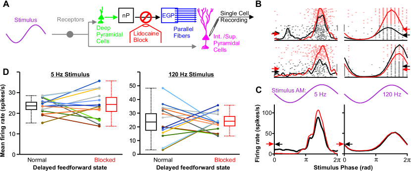
Figure 1: In the ELL of weakly electric fish, firing rate heterogeneity can be increased or decreased by network inputs. A) Schematic of the relevant circuitry of the experimental system. The sinusoidal stimulus’ amplitude is encoded by p-unit electroreceptor which project to pyramidal cells of the ELL. Deep pyramidal cells are the first step of the delayed feedforward pathway which goes through the nucleus praeeminentialis dorsalis (nP), the eminential granularis posterior (EGP) and onto the apical dendrites of superficial and intermediate pyramidal cells of the ELL via granular cell’s parallel fibers. This delayed feedforward pathway can be blocked by lidocaine injection in the fiber bundle that provide inputs to the EGP. B) Example responses of 2 individual pyramidal cells for each stimulus frequency. The average instantaneous firing rate was calculated by Gaussian-convolution (3 ms width) of the binarized spike train and then averaging across cycles of the 15+ sec stimuli. A raster plot of these responses is displayed in the background. Red is used for the responses while the delayed feedforward is blocked; black for responses while it is intact. Arrows show the mean firing rates for the neurons for this stimulus and the gray scale bars near the central edge of the plots represent firing rates changes of 20 Hz. These examples show that the mean firing rates of the neurons can be affected one way or another. Note that, raster plots have a sampling rate of 2 kHz and thus, for 120 Hz sine waves, the raster plot display spike in bins of 1/17th of a cycle. C) Mean instantaneous firing rate for a population of pyramidal cells responding to the 2 sinusoidal stimuli. The instantaneous firing rates of the cycle-histogram shows that the delayed feedforward affects the depth of the modulation of the response to low frequency but not to high frequency stimuli (compare the red and black curves). In both cases the mean firing rate (averaged across time and across neurons) is not dependent on the stimulus frequency or the delayed feedforward block. D) Changes in mean firing rate distribution across the population of cells for low and high frequency responses when the delayed feedforward is blocked. We display the mean firing rate when the delayed feedforward is blocked (right side of the plots) or not (left side of the plots) with two dots of a different color for each neurons linked together by a line. The slope of the line clearly shows that the block cause an increase in firing rate for some neurons and a decrease in others. The box plots show the statistics for this population: mean (central line) standard deviation (box) and range (dotted lines). Clearly, the heterogeneity as measured by the variance is increased by the block for 5 Hz stimuli but decreased for 120 Hz stimuli. Statistics: the 4 populations of firing are normally distributed (Kolmogorov-Smirnov tests: 0.89$>$p$>$0.86). Variance for low frequency varied significantly between blocked and normal condition (F-test p=0.033) and also for high frequency stimuli (p=0.042). Mean firing rate of the whole population (across time and across neurons) did not differ between the blocked vs. normal condition (paired T-test assuming unequal variance; low frequency, p=0.78; high frequency, p=0.91). Our data show significant differences in variance in normal vs. blocked despite our sample size leading to probabilities of finding significant differences of 0.62 and 0.63 as tested with a post-hoc Power Analysis (Faul et al, 2007, 2009) (see Thomas (1997) and Hoenig and Heisey (2001)).

In presenting our model that replicate the experimental effect described above, we first demonstrate that a delayed feedforward spiking neural network model can capture the population firing rate features exhibited in the experimental data, with only 1 major parameter change (sinusoidal frequency) to capture two distinct types of realistic sensory stimuli. For better quantitative matching, we slightly alter the mean and amplitude of the sinusoidal input in the model depending on frequency (see Table 1), which replicates the frequency response profile of these pyramidal cells. Indeed our data shows that the peak of the instantaneous firing is different for low and high frequencies (Fig. 1D). We apply our theory for mean firing rate (trial- and time-averaged) heterogeneity across the population, to the fitted model to determine the relationship of the heterogeneous parameters that captures the firing rate heterogeneity in the data. Finally, we demonstrate the utility of the theory for effective network connectivity with example networks where the probability of connection is structured in such a way to obtain the prescribed correlation between the (heterogeneous) neural attributes derived from the analysis.

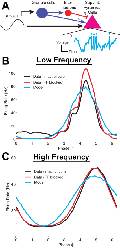
Figure 2: Population firing rates of the data and the delayed feedforward model match. A) Model schematic of the delayed feedforward network. The delayed feedforward model (cyan) not only captures the mean population firing rate of the intact circuit (black) well, but also captures the cycle histogram firing rates for both low (B) and high (C) frequencies. Also shown is the population average cycle histogram from the data when the delayed feedforward input is blocked as in Figure 1B&C. The two frequencies of the afferent stimuli (not shown) in the experiments are 5 Hz and 120 Hz, which are the same two values used in the model (see $\phi$ in $I_{aff}(t)$ in equations (2.1)–(2.1)) and is the main difference (see Methods and Table 1). The trial- and time-averaged population firing rates for the low frequency are: 25.4 Hz (model) and 23.6 Hz (data); for the high frequency: 26.8 Hz (model) and 23.6 Hz (data). Here we set $\varrho(\theta,q)=0$ (see Methods) in the model.

3.1 Adapting the theory for the delayed feedforward network model

Previously, our analysis of heterogeneous recurrent LIF networks provided insights to how the firing rate distribution changed as the relationship between threshold heterogeneity and synaptic variability changed (Ly, 2015). In the weakly electricfish electrosensory system, (sup./int.) pyramidal neurons receive direct feedforward inputs and input that can be qualified as a delayed feedforward input. Fortunately, despite the different types of network, the previously developed theory for recurrent networks can be adapted to feedforward networks (see Appendix A). In this delayed feedforward network, the resulting simplified PDF equations have less dimensions than a recurrent network. The goal of the analysis here is not to accurately capture the time-varying instantaneous firing rates but rather demonstrate the principles for how the relationship between heterogeneous attributes changes the variability in mean firing rates.

In this system, there is a long history of using LIF neural networks to capture salient experimental results and in using computation/analysis to uncover details of electrosensory processing (Doiron et al, 2003; Noonan et al, 2003; Bol et al, 2011; Litwin-Kumar et al, 2012; Mejias et al, 2013). Given these previous results, it is not surprising that our network model was able to capture the population firing rate dynamics with with two distinct stimuli (see Fig. 2). We sought to capture the population firing rate with both low and high frequency inputs by primarily changing one parameter, the frequency of the afferent sinusoidal input: $\phi$ (see equations (2.1)–(2.1)). To insure quantitative accuracy, we also slightly varied the amplitude $\mathcal{A}$ and mean $I_{0}$ of the sinusoidal input (see Table 1). The two frequencies of the sinusoidal input were obtained directly from the experiments where the afferents were driven at 5 Hz and 120 Hz, respectively.

The average population firing rate as a function of the phase of the input frequency is shown for both low frequency (Fig. 2B) and high frequency (Fig. 2C). The model, which has noise (trial-to-trial variability) and the two forms of quenched variability (threshold and synaptic mediated by feedforward inputs), is able to capture the population average response with 2 distinct afferent stimuli (compare the black and cyan curves). Here, the quenched distributions for the threshold heterogeneity $\vec{\theta}$ and synaptic variability $\vec{q}$ were chosen independently with $\varrho=0$ (see equations (5)–(6) and Methods for parameter values). We did not use an optimization routine based on particular algorithms and did not make specific choices about parameters ranges and other parameter attributes; rather, we manually varied the noise levels $\sigma_{P/F}$ and other parameters to match the data. Since the purpose of our computational modeling is to illustrate a principle of network dynamics (specifically effective network connectivity and its relationship with intrinsic excitability/threshold), our results hold equally well with other sets of parameters we used in these same class of models.

The two population of presynaptic (feedforward) cells are relatively simple homogeneous LIF models, with firing rates that depend on the details of the afferent input $I_{aff}(t)$. When $\phi=5\,$Hz, the time-averaged firing rates are $\langle r^{E}(t)\rangle_{t}=8.5$ Hz and $\langle r^{I}(t)\rangle_{t}=19.4$ Hz; when $\phi=120\,$Hz, $\langle r^{E}(t)\rangle_{t}=9.1$ Hz and $\langle r^{I}(t)\rangle_{t}=14.1$ Hz.

Once adapted and fitted, we calculate the net feedforward input to the (sup./int.) pyramidal cells and find that they are dominated by excitation (for all cells and all parameters). This strong drive that is net excitatory is crucial for determining which limit to take in the asymptotic calculation in Appendix A. In Appendix A (equation (28)), by taking the limit of large voltage values, we show that the firing rate heterogeneity (std. dev.) is captured qualitatively by:

$$\sigma\left(\vec{\nu}\right)\approx C\sqrt{\frac{1}{N-1}\sum_{j=1}^{N}\left(\frac{q_{j}}{\theta_{j}}-\mu\left(\frac{\vec{q}}{\vec{\theta}}\right)\right)^{2}}$$ (7)

where $\mu\left(\frac{\vec{q}}{\vec{\theta}}\right)=\frac{1}{N}\displaystyle\sum_{j=1}^{N}\frac{q_{j}}{\theta_{j}}$. In the analysis, we focus on a specific limit of the reduced firing rate equations rather than dealing with a multidimensional partial differential equation.

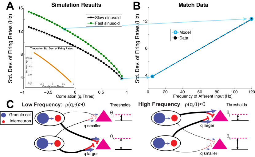
Figure 3: Model prediction: the effective network input strength depends on the afferent stimuli and the excitability of the target neuron. A) Simulations of the firing rate standard deviations in the delayed feedforward networks as the correlation between $\vec{q}$ and $\vec{\theta}$ vary with low (black) and high (green) frequency sinusoidal input. Inset: The standard deviation of firing rates as the correlation between $\vec{q}$ and $\vec{\theta}$ varies, using equation (7). B) To capture the different firing rate standard deviations, consider different correlations of $(q,\theta)$ for each stimuli. In the data, with a low frequency (5 Hz) stimuli, there were 15 neurons with trial averaged firing rate standard deviation of 3.8 Hz (population average of 23.6 Hz); with a high frequency (120 Hz), there were 15 neurons with trial averaged firing rate standard deviation of 12.3 Hz (population average of 23.6 Hz). In the model (cyan dots), with the same parameters as in Fig. 2 were used, but now the correlation $\varrho$ is allowed to vary. For the low frequency, $\varrho=0.9$ gives the best approximation to the firing rate standard deviation of the data among the $\varrho$ mesh values considered. For the high frequency, $\varrho=-0.2$ gives the best approximation to the firing rate standard deviation of the data. C) Cartoon of a small sub network to illustrate how intrinsic threshold $\theta$ of 2 neurons is related to effective network input strength $q$ that consists of both excitatory and inhibitory inputs. For low frequencies, $\varrho(\theta,q)>0$ so that neurons with smaller $\theta$ tend to have smaller effective network input $q$ (and vice-versa). With high frequencies, $\varrho(\theta,q)<0$ so that neurons with smaller $\theta$ tend to have larger effective network input $q$ (and vice-versa).

Figure 3A demonstrates how the firing rate standard deviations change as the correlation $\varrho$ between threshold heterogeneity and synaptic variability vary. When $\varrho<0$, larger $\theta_{j}$ tend to occur with smaller $q_{j}$, so the maximum of $q/\theta$ is amplified (big times big) and the minimum is diminished (small times small), resulting in relatively large heterogeneity. When $\varrho>0$, larger $\theta_{j}$ tend to occur with larger $q_{j}$ so both the variance of $q/\theta$ is smaller (small times big minus big times small), resulting in a relatively small heterogeneity.

Intuitive Understanding of Figure 3A. A priori, guessing how the firing rate heterogeneity changes as the correlation of $\vec{\theta}$ and $\vec{q}$ varies is difficult and depends on models, regimes, etc. (see Ly (2015) where the firing rate range depends nonlinearly on intrinsic and network heterogeneity). However, since the feedforward input is effectively excitatory in the models and regimes here, the results in Figure 3A can be understood as follows. If cells with high threshold have weak inputs (i.e., smaller $q$), they will have low rates; at the same time, cells with low thresholds have strong inputs (i.e., larger $q$), they will have high rates – together, the whole population will have a broad distribution of rates. If, on the other hand, those cells with high thresholds receive strong inputs and those with low threshold receive weak inputs, then the distribution will be narrower. The opposite trend would occur if the feedforward input is net inhibitory.

Since the experimental data shows that the delayed feedforward input is crucial for observing less firing rate heterogeneity with lower frequencies than with higher frequencies (Fig. 1B), our model is applicable because the structure of this delayed feedforward input strongly effects the firing rates. Indeed, the theory applied to these parameters (Fig. 3A, inset) is validated in the large spiking network model (Fig. 3A). Here, the firing rate standard deviations are plotted while $\varrho(\vec{\theta},\vec{q})$ is varied while keeping the mean and variance (among the $N$ target cells) fixed. There are two curves because two different sinusoidal frequencies $\phi$ were used: 5 Hz in black and 120 Hz in green. We remark that the statistics of the feedforward inputs remain the same throughout the various correlation values $\varrho(\vec{\theta},\vec{q})$, but since there is (colored) noise $\sigma_{F}\eta_{l}$, there are minor deviations for each simulated network due to finite simulations.

3.2 Model prediction: strength of effective delayed feedforward inputs depends on stimuli

A natural model prediction from these modeling results (Fig. 3B) is that the effective delayed feedforward input strength is structured in a stimulus-dependent manner. With lower frequency afferent inputs, we use the model to predict that the pyramidal cells with higher thresholds (intrinsically less excitable) receive overall stronger delayed feedforward excitatory and inhibitory input than cells with lower thresholds (more excitable); that is, $\varrho>0$. With higher frequency afferent inputs, the model predicts that pyramidal cells with higher threshold (intrinsically less excitable) receive overall weaker delayed feedforward excitatory and inhibitory input than cells with lower thresholds ($\varrho<0$).

Figure 3B shows the firing rate standard deviation from the experimental data (as a function of the dominant sinusoidal frequency), compared with the fitted model where we see different firing rate standard deviations depending on $\varrho$. With the low frequency, we plot the firing rate standard deviation with the ‘best’ corresponding $\varrho$ that is closest to the firing rate standard deviation from the data ($\varrho=0.9$, recall the black curve in Fig. 3C) in cyan. With the high frequency, again we plot the firing rate rate with the ‘best’ corresponding $\varrho$, which is $\varrho=-0.2$ (green curve in Fig. 3A) in cyan. Given the good match between model and data, the application of the theory clearly demonstrates:

• The correlation $\varrho$ is significant in controlling the firing rate heterogeneity

• The specific network input strength (or structure) depends on both stimulus and targeted neuron

The difference in firing rate heterogeneity cannot be attributed to the sinusoidal frequency $\phi$ in this model because we have already seen that it does not vary much with the two different sinusoidal inputs (Fig. 3A).

Figure 3C shows a schematic picture of the model prediction for two pyramidal cells with lower and higher thresholds receiving feedforward inputs. This prediction’s viability relies on the network providing different sets of inputs for different stimulus frequencies – a fact supported by previous experimental results (Bol et al, 2011). The thickness of the arrows indicate how strong the effective network input ($q$) is from both presynaptic E and I cells. This model prediction is a statistical statement about the aggregate population and not about individual cells. For example, the theory certainly allows for cells with higher thresholds to have larger effective network inputs with high frequency inputs (appearing to violate $\varrho<0$), but the correlation being negative (in this case) means these cases will happen less often than the other case.

3.3 Linking theory to neural architecture

In the prior section we showed a direct application of the theory where the parameters $(\theta_{j},q_{j})$ were manipulated in the computational model, resulting in firing rate standard deviations captured by our analysis. In this section, we apply the theory in a different way and link it with the architecture of a neural network. A motivating reason for this is that many sensory systems can encounter both low and high frequency stimuli, and it is conceivable that it may need to process both low and high frequency stimuli in rapid succession. Thus, the effective network input strength $\vec{q}$ may not be able to change fast enough, which would seemingly weaken our theory. We present an alternative application of our theory using network coupling to address this.

The neural network model we consider here has fixed heterogeneity values $(\vec{\theta},\vec{q})$ for the target pyramidal cells, and we set $\varrho(\vec{\theta},\vec{q})=0$ (although we will see this is not necessary). The network is designed so that the effective correlation between $\vec{\theta}$ and $\vec{q}$ are as before (i.e., $\varrho>0$ for smaller $\phi$ and $\varrho<0$ for larger $\phi$). Networks in the previous sections have a 20% connection probability, so some cells do not receive network inputs; by effective we mean that pyramidal cells that are actually connected the delayed feedforward have this $\varrho$. Here, only a subset of presynaptic granule cells will be activated and respond (i.e., spike) to sinusoidal input (previously they all responded equally), and different groups of these granule cells will respond depending on the sinusoidal frequency $\phi$ (see Fig. 5A and Appendix B for details). Indeed, there is evidence based on recordings and theory for frequency tuning of granule cells in the ELL (Bol et al, 2011). By construction, pyramidal cells are differentially activated by delayed feedforward input, but note that as before, all pyramidal cells receive the same afferent sinusoidal input $I_{aff}$. The connectivity rules for the delayed feedforward network will no longer be random (Erdős-Rényi graph, see Figure 5B) but rather the activated presynaptic cells have a higher probability of connecting to pyramidal cells that result in the desired $\varrho$; Figure 4A shows a cartoon schematic of this idea. In implementing this idea, we make the assumption that the effective $\varrho(\vec{\theta},\vec{q})$ varies continuously from a high (positive) value to low (negative) value as $\phi$ increases. There are numerous ways to effectively have various $\varrho$ values in the pyramidal cells, and we only present 2 instances of the network (see Appendix B for connectivity rules and other details). Figure 4B illustrates the connectivity rules for Network 1: the activated presynaptic cells at a low frequency have a higher probability of connection to the red cells on a diagonal band in $(\vec{q},\vec{\theta})$ space (color bar represents actual number of inputs with various $\phi$). The reason for this diagonal band with positive slope is that the effective $\varrho$ will be positive. As $\phi$ increases, other sets of presynaptic cells are activated and the probability of connection is again higher for target cells that are in the red band. Figure 4C illustrates the connectivity rules for Network 2 that are similar to the previous network except the region is different. The activated presynaptic cells at a low frequency have a higher probability of connection to the red cells that form two triangular wedges in $(\vec{q},\vec{\theta})$ space. Again, as $\phi$ increases, other sets of presynaptic cells are activated and the probability of connection is higher for cells that are in the red band.

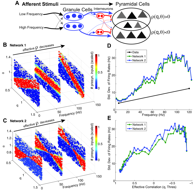
Figure 4: Using the theory to capture the firing rates standard deviations in the data with fixed $(\vec{\theta},\vec{q})$, with $\varrho(\vec{\theta},\vec{q})=0$. A) Demonstrates how the theory can be used to get different firing rates standard devaitions. Depending on frequency on the afferent stimulus, selective activation of granule cells can provide effectively more presynaptic input to the desired set of pyramidal cells that have a specific $\varrho(\vec{\theta},\vec{q})$ (i.e., $\varrho>0$ for low frequencies and $\varrho<0$ for higher frequencies). B) Network 1: a particular network architecture that captures the desired $\varrho$, for fixed $(\vec{\theta},\vec{q})$, shown for three different frequencies. The coloring indicates a measure of the effective input (red is more, blue is less): (number of presynaptic inputs from granule cells)$\times$(Probability granule cell fires), scaled to have values in [0,1]. C) Network 2: another network architecture that captures the desired $\varrho$. In both networks, we assume $\varrho$ varies continuously as the frequency increases; this assumption is not necessary and is only made to demonstrate the utility of the theory. D) Comparing how the firing rate heterogeneity (measured by standard deviation) with frequency in both network models and in the experimental data. Consistent with the theory, we see the heterogeneity generally increases with frequency. In both network models, since the total numbers of granule and pyramidal cells are kept fixed (see Table 1), the conductance values here are exactly the same as the previous figures. E) The firing rate standard deviation as a function of the effective $\varrho$ (reverse scale, positive is left, negative is right) from the two networks is consistent with the theoretical analysis.

In these two networks (Network 1, 2), there are overall less presynaptic cells activated than before (we kept the same $N_{f}=100$ and $N=1000$), but even keeping the same conductance strengths $(s_{e},s_{i})$ happened to result in firing rates that are comparable to the previous model (Fig. 3). In general, the conductance strengths $(s_{e},s_{i})$ may need to change to account for different presynaptic cell activation. With a fixed architecture, afferent sinusoidal input is provided to all populations as before and only the frequency $\phi$ is varied (with selective activation of presynaptic granule cells). We simply linearly interpolate the values of the amplitude $\mathcal{A}$ and mean $I_{0}$ sinusoidal input between 5 Hz and 120 Hz (recall the slightly different values in Table 1). The resulting firing rate standard deviations (Fig. 4D) are again described by our reduced analytic descriptions (Eq. (7)). Specifically, the effective correlation $\varrho$, which in this case was attributed to a particular frequency $\phi$, is the determining factor in the firing rate standard deviation. Figure 4E shows this directly; the firing rate standard deviations from these two networks are plotted as a function of effective correlation (reverse scale on x-axis) and again the standard deviation is larger with $\varrho<0$ than $\varrho>0$. There is a drop in firing rate range in Fig. 4E around -1 due to it being a hard bound on correlation; but there is also a drop in Fig. 4D after $\sim 100$ Hz following a relatively steady (yet noisy) increase in the firing rate range in both networks. This is likely because the scheme we chose to illustrate this principle did not insure that all frequencies received the same total sinusoidal drive, together with the structured connectivity rules resulted in different ranges of inputs (across the population) that varied with frequency. It is difficult to insure strict monotonicity in the firing rate range because of all the interacting components, yet our theory is valuable in understanding how this complicated statistic modulates. Unlike the previous neural network, we were able to obtain different firing rate standard deviations with the same fixed $(\vec{\theta},\vec{q})$ and fixed connectivity that is structured as opposed to completely random.

We chose to illustrate our result with two networks to show that although there are differences in the actual range of firing rates that depend on numerous factors (network connectivity rules, input parameters, etc.), the qualitative results of our theory holds and thus we expect the results to hold with other prescribed network configurations.

Our model and the results of Figure 4 demonstrate the value of our theoretical results. These theoretical results not only enable a specific prediction about how the effective feedforward inputs are related to excitability, but can also be applied to predict probability of connections based on intrinsic excitability and frequency tuning.

4 Discussion

We have adapted and applied a theory for firing rate heterogeneity in recurrent networks to a delayed feedforward network, and used data from the electrosensory system of the weakly electric fish to motivate this theoretical application and constrain the model. Our data shows that firing rate heterogeneity is larger for higher frequency sinusoidal input (courtship of opposite sex) than with lower frequency sinusoidal input (antagonizing signal with same sex animals), and that this difference in heterogeneity is determined by the delayed feedforward. Our theory and computational models predict that, in order to account for the observed firing rate statistics, the effective network connectivity is dynamically modulated depending on stimulus features. Our work uses theoretical analysis to specifically predict how the interactions of neural attributes (threshold heterogeneity and synaptic strengths) lead to heterogeneous firing rate statistics with various stimuli. These results may be generalizable to other feedforward neural networks.

Our theoretical analysis replicates a fairly simple configuration were the correlation between synaptic strength and threshold can influence population heterogeneity. Our analysis reveals that this relationship is non-trivial in that it is a nonlinear function of synaptic strength divided by threshold that controls the firing rate heterogeneity across the population rather than how these individual quantities alter a cell’s firing rate (see Fig. 7 in Appendix C for how these individual quantities are related to firing rate).

Other cellular or network features certainly effect the firing rate heterogeneity, but we focus on threshold heterogeneity because threshold is known to be important in this system (Middleton et al, 2009), and other cellular attributes can be related to the threshold in the leaky integrate-and-fire model (Mejias and Longtin, 2012, 2014). Besides the previously mentioned reasons for the existence and importance of different synaptic strengths, our data shows that delayed feedforward input activity from the specific network of granule cells significantly affects the firing rate distribution because when it is blocked, the firing rate heterogeneity does not vary much. Several other attributes of sensory neurons, and the distribution of their heterogeneity will influence the way they encode information (tuning, non-linearity, plasticity, to name only a few). Investigating how network dynamic influences these heterogeneities is a rich research direction for future studies.

Although the fitted model was best described by the ‘rhythmic’ regime where the presynaptic inputs were large, the theory in Ly (2015) also accounts for asynchronous regimes where the presynaptic inputs are weaker and background fluctuations significantly affects spiking. In those regimes, the relationship between the heterogeneous attributes lead to different firing rate heterogeneity than the ‘rhythmic’ regimes. Thus, the experimental predictions can be reexamined and potentially augmented if other fitted models happen to operate in a different regime.

Whether our theoretical predictions are verified in the weakly electric fish are yet to be determined, however we discuss various possibilities here. An alternative explanation for the modulation of firing rate heterogeneity is that the heterogeneity of the presynaptic firing rate could modulate with stimulus (in our models the presynaptic firing rates are statistically homogeneous) and the superficial pyramidal cells would inherit this heterogeneity. However, this would not explain all of the experimental data: with the afferent input strength being identical in all cases, blocking the delayed feedforward input increased the firing rate heterogeneity for low frequencies (and decreased it for high frequencies). Clearly, the delayed feedforward input cannot simply contribute to the cells’ firing rate heterogeneity, otherwise blocking the feedback would systematically reduce heterogeneity by removing a source of variability. Instead, our model shows that firing rate heterogeneity can either increase or decrease simply but varying the correlation between network input strength and the cells’ excitability (threshold). Experimental verification that this mechanism does indeed play a role in the ELL would require a thorough set of experiments, probably involving both in-vitro and in-vivo recording. We know that this mechanism is not the only one affecting firing rate heterogeneity in the ELL. For example, a previous study showed that the delayed feedforward input interacts with the burst-generating mechanism to produced stereotyped responses (less heterogeneous) during low-frequency stimulation (Marsat and Maler, 2012). This study can, in fact, fit the theory presented here. If one considers bursting as a source of intrinsic excitability, that paper showed strong positive network input interacts with this intrinsic excitability, the implication being that a positive correlation between the two would lead to strong stereotyped bursts (low heterogeneity). Clearly, ELL pyramidal cells have many more properties than are being explicitly modeled here, but it is precisely the reason that makes our theory so general and applicable to a wide variety of systems.

We focus specifically on firing rate heterogeneity because it is the first order statistic and crucial in understanding the mechanisms that lead to efficient coding. The effects of heterogeneity of neural attributes on coding and dynamics of neural networks is important and has been studied by numerous authors both in a general theoretical framework (Hermann and Touboul, 2012; Mejias and Longtin, 2012; Hunsberger et al, 2014; Mejias and Longtin, 2014) and in specific neural systems (Shamir and Sompolinsky, 2006; Chelaru and Dragoi, 2008; Marsat and Maler, 2010; Marsat et al, 2012). Our results differ from these studies in many ways, but largely because i) we account for two heterogeneous attributes, ii) we make a specific prediction about synaptic strengths depending on the pyramidal (target) cells and stimulus features. The results here may be applicable to other systems given how common feedforward pathways are and how well spiking neuron models can capture the statistics of neural network activity.

Firing rate heterogeneity is just one statistical measure of the network response, and there are other measures that may also be crucial in the context of neural coding. The spike coherence of the response with the afferent stimuli is commonly used in the electrosensory system (Chacron et al, 2005; Mehaffey et al, 2008; Middleton et al, 2009), and thus an important future direction is how the heterogeneity of the firing rate in time affects the efficiency of coding. In addition to the afferent sinusoidal input, communication signals in electric fish also consist of brief chirps. However, the predominant electrical signal in time is the nearly sinusoidal input that we have considered. The afferent sinusoidal activity without the transient chirp at the very least sets the stage for the neural network to readily decode the chirp input, and is thus an important component (Marsat and Maler, 2012). Another potentially important measure is the second order statistics, or the spike count correlation, of the pyramidal cells (Averbeck et al, 2006; Cohen and Kohn, 2011; Doiron et al, 2016). A few studies have recently considered how spike count correlation in the ELL might effect coding of signals: Litwin-Kumar et al (2012) considered how local/global stimulation alters correlation at different time windows of superficial pyramidal cells, Simmonds and Chacron (2015) considered the how noise (and signal) correlation modulates with granule cell (parallel fiber) input, and Chacron and Bastian (2008) showed how the noise correlation of these neurons depends on stimulus type and firing pattern (bursts). Theoretical analyses of such measures when focusing on heterogeneity are complicated (Josić et al, 2009; Ecker et al, 2011; Ly et al, 2012) and beyond the scope of this current paper.

Appendix A: Asymptotic calculation for the relative standard deviation of firing rate distribution

The asymptotic calculations were all based on an expression for the firing rate of an individual neuron via the PDF or Population Density framework that has been commonly used in spiking models in cortex models (Knight, 1972; Wilbur and Rinzel, 1982; Fourcaud and Brunel, 2002; Brunel and Latham, 2003; Tranchina, 2009) and other areas (Barna et al, 1998; Brown et al, 2004; Huertas and Smith, 2006). In addition to the firing rate, this framework has been useful in calculating many statistical quantities of the spike train (Brunel et al, 2001; Richardson, 2007, 2008) and to study the stability of coupled networks (Knight, 1972; Abbott and van Vreeswijk, 1993; Brunel and Hakim, 1999; Gerstner, 2000; Ly and Ermentrout, 2010). It can also be employed as a time saving computational tool (Nykamp and Tranchina, 2000; Omurtag et al, 2000; Apfaltrer et al, 2006; Ly and Tranchina, 2007). We focus on the standard deviation of firing rates and use the framework to gain analytic insight into the dynamics.

To employ the framework and for feasibility, we make some technical assumptions:

1. the (average) population firing rate is a good approximation to the presynaptic input rate with random connectivity

2. a single p.d.f. function is adequate to describe a single population’s activity

3. the heterogeneity is driven by $(q_{j},\theta_{j})$ only

The complexities that arise in a recurrent network (nonlinear PDF equation) never came about (Ly, 2015) in our specific analysis because of the networks here are delayed feedforward networks. Moreover, the resulting PDF equations have lower dimensions than a recurrent network. We begin by writing down the probability density function for both (E and I) presynaptic populations that provide delayed feedforward input.

$$\rho^{E}(v,\eta,t)\,dvd\eta=\Pr\left(\hbox{presyn E cell}\in\{(v,v+dv)\cap(\eta,\eta+d\eta)\}\right)$$

$$\rho^{I}(v,\eta,t)\,dvd\eta=\Pr\left(\hbox{presyn I cell}\in\{(v,v+dv)\cap(\eta,\eta+d\eta)\}\right)$$

The PDF equations for the presynaptic E population are:

$$\frac{\partial\rho^{E}}{\partial t} = -\frac{\partial}{\partial v}\left\{J_{V}(v,\eta,t)\right\}-\frac{\partial}{\partial\eta}\left\{J_{\eta}(v,\eta,t)\right\}$$

$$J_{V}(v,\eta,t) = \frac{1}{\tau_{m}}\left[I_{aff}(t)-v+\sigma_{F}\eta\right]\rho^{E}$$ (8)

$$J_{\eta}(v,\eta,t) = \frac{1}{\tau_{n}}\left[-\eta\rho^{E}-\frac{1}{2}\frac{\partial\rho^{E}}{\partial\eta}\right]$$ (9)

$$J_{V}(1,\eta,t) = J_{V}(0,\eta,t+\tau_{fref})$$ (10)

$$r^{E}(t) = \int_{-\infty}^{\infty}J_{V}(1,\eta,t)\,d\eta$$ (11)

where $r^{E}(t)$ is the population firing rate. The presynaptic I population is similar but lacks direct sinusoidal input:

$$\frac{\partial\rho^{I}}{\partial t} = -\frac{\partial}{\partial v}\left\{J_{V}(v,\eta,t)\right\}-\frac{\partial}{\partial\eta}\left\{J_{\eta}(v,\eta,t)\right\}$$

$$J_{V}(v,\eta,t) = \frac{1}{\tau_{m}}\left[-v-g_{EE}(t)(v-\mathcal{E}_{E})+\sigma_{F}\eta\right]\rho^{I}$$ (12)

$$J_{\eta}(v,\eta,t) = \frac{1}{\tau_{n}}\left[-\eta\rho^{I}-\frac{1}{2}\frac{\partial\rho^{I}}{\partial\eta}\right]$$ (13)

$$J_{V}(1,\eta,t) = J_{V}(0,\eta,t+\tau_{fref})$$ (14)

$$r^{I}(t) = \int_{-\infty}^{\infty}J_{V}(1,\eta,t)\,d\eta$$ (15)

For simplicity, we assume the synaptic conductances of the target (superficial pyramidal) cells can be averaged in time (see equation (2.1)):

$$g_{EE}(t)=s_{EE}\int r^{E}(t-t^{\prime})K(t^{\prime})\,dt^{\prime}$$

$$g_{e}(t)=s_{e}\int r^{E}(t-t^{\prime})K(t^{\prime})\,dt^{\prime}$$

$$g_{i}(t)=s_{i}\int r^{I}(t-t^{\prime})K(t^{\prime})\,dt^{\prime}$$

where $K$ is the alpha function kernel:

$$K(t)=H(t)\frac{\alpha}{\frac{\tau_{d}}{\tau_{r}}-1}\Big{[}e^{-t/\tau_{d}}-e^{-t/\tau_{r}}\Big{]}$$

and $H(t)$ is the Heaviside step function and $\tau_{r}<\tau_{d}$ (a common assumption in models of synapses). This kernel is unconventional in that $\int_{-\infty}^{\infty}K(t)\,dt=\alpha\tau_{r}$ and $\neq 1$.

Finally, the PDF for the target cells:

$$\rho(v,\eta,t)\,dvd\eta=\Pr\left(\hbox{pyramidal cell}\in\{(v,v+dv)\cap(\eta,\eta+d\eta)\}\right)$$

are described by:

$$\frac{\partial\rho}{\partial t} = -\frac{\partial}{\partial v}\left\{J_{V}(v,\eta,t)\right\}-\frac{\partial}{\partial\eta}\left\{J_{\eta}(v,\eta,t)\right\}$$

$$J_{V}(v,\eta,t) = \frac{1}{\tau_{m}}\Big{[}I_{aff}(t)-v-q_{j}g_{e}(t-\tau_{del})(v-\mathcal{E}_{E})-q_{j}g_{i}(t-\tau_{del})(v-\mathcal{E}_{I})+\sigma_{P}\eta\Big{]}\rho$$ (16)

$$J_{\eta}(v,\eta,t) = \frac{1}{\tau_{n}}\left[-\eta\rho-\frac{1}{2}\frac{\partial\rho}{\partial\eta}\right]$$ (17)

$$J_{V}(1,\eta,t) = J_{V}(0,\eta,t+\tau_{ref})$$ (18)

$$r_{j}(t) = \int_{-\infty}^{\infty}J_{V}(\theta_{j},\eta,t)\,d\eta.$$ (19)

The firing rate $r_{j}(t)$ is not a population firing rate, but rather the firing rate of the $j^{th}$ neuron in the population. We implicitly assume that the only difference between cells is given by the two heterogeneous parameters: $(\theta_{j},q_{j})$.

Our goal is not to capture the time-varying firing rates (which are still difficult even with these assumptions because of the three coupled PDEs that each have 2 spatial dimensions and time), but rather we are interested in the trial- and time-averaged firing rates. This enables a compact expression for how the heterogeneity ($\vec{\theta},\vec{q}$) relationship controls the heterogeneity of steady-state firing rates. We have:

$$\nu_{j}:=\langle r_{j}(t)\rangle_{t}$$ (20)

We approximate

$$\Big{\langle}\int_{-\infty}^{\infty}I_{aff}(t)\rho(v,\eta,t)\,d\eta\Big{\rangle}_{t}\approx\int_{-\infty}^{\infty}\langle I_{aff}(t)\rangle_{t}\langle\rho(v,\eta,t)\rangle_{t}\,d\eta,$$ (21)

and similarly for the expressions with $g_{e/i}$. This leads to:

$$\nu_{j}\approx\frac{1}{\tau_{m}}\Big{[}I_{0}-\theta_{j}+\bar{g}_{E}(\mathcal{E}_{E}-\theta_{j})-\bar{g}_{I}(\theta_{j}-\mathcal{E}_{I})\Big{]}f(\theta_{j})+\frac{\sigma_{P}}{\tau_{m}}\int_{-\infty}^{\infty}\eta\rho(\theta_{j},\eta)\,d\eta$$ (22)

where $f(v)=\int\rho(v,\eta)\,d\eta$ is the steady-state marginal voltage distribution (equal to the time-average, assuming ergodic theorems apply), and $\bar{g}_{E}=\alpha\tau_{r}\langle r^{E}(t)\rangle_{t}$, $\bar{g}_{I}=\alpha\tau_{r}\langle r^{I}(t)\rangle_{t}$. One could simply numerically simulate these equations, but there is not much analytic insight gained in understanding how ($\vec{\theta},\vec{q}$) and $\varrho(\vec{\theta},\vec{q})$ alter the firing rate standard deviation. In applying dimension reduction methods, there are issues that arise in trying to accurately capture the firing rate (Ly and Tranchina, 2007). Thus, we apply a simple (quantitatively inaccurate) dimension reduction method where we assume $\eta$ is frozen and average over the resulting firing rate (Moreno-Bote and Parga, 2006; Nesse et al, 2008; Hertäg et al, 2014; Nicola et al, 2015; Ly, 2015). We also ignore the effects of the refractory period $\tau_{ref}$ . The firing rate is then simply:

$$\nu_{j}(\theta_{j},q_{j}) \approx \int_{-\infty}^{\infty}\nu_{det}(\theta_{j},q_{j};\eta)\frac{e^{-\eta^{2}}}{\sqrt{\pi}}\,d\eta$$ (23)

$$\nu_{det}(\theta_{j},q_{j};\eta) = \begin{cases}0,&\text{if }\frac{q(\bar{g}_{E}\mathcal{E}_{E}+\bar{g}_{I}\mathcal{E}_{I})+\sigma_{P}\eta+I_{0}}{1+q(\bar{g}_{E}+\bar{g}_{I})}\leq\theta_{j}\\ \frac{1+q(\bar{g}_{E}+\bar{g}_{I})}{\tau_{m}\log\left(\frac{q(\bar{g}_{E}\mathcal{E}_{E}+\bar{g}_{I}\mathcal{E}_{I})+\sigma_{P}\eta+I_{0}}{q(\bar{g}_{E}\mathcal{E}_{E}+\bar{g}_{I}\mathcal{E}_{I})+\sigma_{P}\eta+I_{0}-\theta(1+q(\bar{g}_{E}+\bar{g}_{I}))}\right)},&\text{if }\frac{q(\bar{g}_{E}\mathcal{E}_{E}+\bar{g}_{I}\mathcal{E}_{I})+\sigma_{P}\eta+I_{0}}{1+q(\bar{g}_{E}+\bar{g}_{I})}>\theta_{j}\end{cases}$$ (24)

The parameters $(\theta_{j},q_{j})$ determine how one $\nu_{j}$ differs from another; to see how the combined effects of threshold heterogeneity and synaptic variability alter $\nu_{j}$, we consider a specific limit. That is, the simulations indicate that the the net conductance are large in the fitted model (Fig. LABEL:fig:chooseThry), thus, we consider the large firing rate limit of the term in the integrand $\nu_{det}$, to get:

$$\tau_{m}\nu_{det}(\theta_{j},q_{j}) = \frac{1+q_{j}(\bar{g}_{E}+\bar{g}_{I})}{\log\left(\frac{q_{j}(\bar{g}_{E}\mathcal{E}_{E}+\bar{g}_{I}\mathcal{E}_{I})+\sigma_{p}\eta+I_{0}}{q_{j}(\bar{g}_{E}\mathcal{E}+\bar{g}_{I}\mathcal{E}_{I})+\sigma_{p}\eta+I_{0}-\theta_{j}(1+q_{j}(\bar{g}_{E}+\bar{g}_{I}))}\right)}$$ (26)

$$= \frac{q_{j}}{\theta_{j}}(\bar{g}_{E}\mathcal{E}_{E}+\bar{g}_{I}\mathcal{E}_{I})+\frac{\sigma_{p}\eta+I_{0}}{\theta_{j}}-\frac{1}{2}(1+q_{j}(\bar{g}_{E}+\bar{g}_{I}))$$

$$-\frac{(1+q_{j}(\bar{g}_{E}+\bar{g}_{I}))^{2}\theta_{j}}{12[q_{j}(\bar{g}_{E}\mathcal{E}_{E}+\bar{g}_{I}\mathcal{E}_{I})+\sigma_{p}\eta+I_{0}-\theta_{j}(1+q_{j}(\bar{g}_{E}+\bar{g}_{I}))]}$$

$$+O\left(z^{2}(1+q_{j}(\bar{g}_{E}+\bar{g}_{I}))\right)$$

$$\hbox{where }z := \theta_{j}\frac{1+q_{j}(\bar{g}_{E}+\bar{g}_{I})}{q_{j}(\bar{g}_{E}\mathcal{E}_{E}+\bar{g}_{I}\mathcal{E}_{I})+\sigma_{p}\eta+I_{0}-\theta_{j}(1+q_{j}(\bar{g}_{E}+\bar{g}_{I}))}$$ (27)

This calculation is very similar to the one in Ly (2015). The key term is the first term in equation (26),

$$\frac{q_{j}}{\theta_{j}}(\bar{g}_{E}\mathcal{E}_{E}+\bar{g}_{I}\mathcal{E}_{I})$$

which is the dominant term assuming $\nu_{det}$ is large. Substituting the expansion (26) into the integral approximation (23) only changes terms with $\eta$ in them (i.e., the dominant term does not change and the term $\sigma_{P}\eta/\theta_{j}$ evaluates to 0). This shows analytically that the term $q_{j}/\theta_{j}$ is the dominant source of firing rate heterogeneity, and that we can approximate:

$$\sigma\left(\vec{\nu}\right)\approx C\sqrt{\frac{1}{N-1}\sum_{j=1}^{N}\left(\frac{q_{j}}{\theta_{j}}-\mu\left(\frac{\vec{q}}{\vec{\theta}}\right)\right)^{2}}$$ (28)

where $\mu\left(\frac{\vec{q}}{\vec{\theta}}\right)=\frac{1}{N}\displaystyle\sum_{j=1}^{N}\frac{q_{j}}{\theta_{j}}$.

Appendix B: Details of network connectivity and model in section 3.3

We used two networks, which we generically labeled as Network 1 and Network 2 (see Fig. 4), to help demonstrate the utility of the theory for firing rate standard deviations with different architectures than random (Erdős-Rényi graph). We first describe how we selectively activate the granule cells that provide delayed feedforward input to the pyramidal cells, and then describe the connectivity rules for each network.

Selective activation of granule cells. Instead of providing constant sinusoidal drive to each of the $2N_{f}$ presynaptic granule cells, the afferent stimuli $I_{aff}(t)=I_{0}+\mathcal{A}\sin(2\pi\phi t)$ is scaled by a parameter $C(l,\phi)$:

$$I_{aff}(t)=C(l,\phi)\Big{\lceil}I_{0}+\mathcal{A}\sin(2\pi\phi t)\Big{\rceil}^{+}$$

that depends on both frequency $\phi$ and the index of cell $l\in\{1,2,\dots,N_{f}\}$ ($2N_{f}$ total because there are both excitatory and inhibitory presynaptic cells). The afferent stimuli to the target pyramidal cells is the same as before (see equation (2.1)). Before providing the formula for $C(l,\phi)$, we note that the strength of the sinusoidal drive will follow a (scaled) beta distribution where the location of the maximum value increases as $\phi$ increases. We use:

$$C(l,\phi)=1.5\frac{x(l)^{19}(1-x(l))^{21.52*\frac{125}{\phi}-21}}{\displaystyle\max_{1\leq l\leq N_{f}}\beta(l,\phi)}$$ (29)

where

$$\beta(l,\phi) = x(l)^{19}(1-x(l))^{21.52*\frac{125}{\phi}-21}$$

$$x(l) = \frac{2.5\,\hbox{Hz}}{125\,\hbox{Hz}}(\lceil l/4\rceil-1/2)$$

The term $\beta(l,\phi)$ is simply the numerator of the fraction in $C(l,\phi)$ so that $C(l,\phi)\in(0,1.5)$. The variable $x(l)$ is the end result of mapping the $l^{th}$ presynaptic neuron to one of 50 frequencies (equally spaced by 2.5 Hz from 1.25 Hz to 123.75 Hz) and normalizing by 125 Hz. Here we are assuming $\phi\in[0,125]$ Hz so that $x(l)\in(0,1)$; other frequencies can easily be incorporated with minor adjustments to the above formulas. Finally, notice that in $x(l)$, we have the term: $\lceil l/4\rceil$, which denotes rounding up after dividing by 4; this essentially groups presynaptic neurons into groups of size 4 that receive the same sinusoidal drive. Figure 5A illustrates how the sinusoidal drive to the presynaptic cells, indexed by $l$, vary with several fixed frequencies $\phi$.

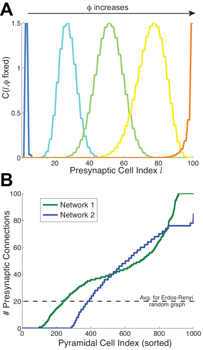
Figure 5: Activation of presynaptic cells depends on the frequency of the afferent sinusoidal input. A) The strength of the sinusoidal input $C(l,\phi)$ (see equation (29)) for particular frequencies; from left to right, $\phi=3.75,33.75,63.75,93.75,123.75$ Hz. B) Showing the number of presynaptic connections (out of $N_{f}=100$) for each of the $N=1000$ target pyramidal cells (sorted from smallest to largest) in both networks. Notice the structure of the connectivity, compared to completely random connectivity (black dash line, with 20% connection probability).

Connectivity rules for Network 1. To illustrate the usefulness of the theory, we implemented a static delayed feedforward network with fixed $(\vec{\theta},\vec{q})$ and certain connectivity rules (see below). The presynaptic granule cells are indexed as before via $l$, and the target pyramidal cells by $j$. Recall that both $E$ and $I$ cells in the presynaptic population have the same connectivity for simplicity.

Each pyramidal cell $j$ has an associated $(\theta_{j},q_{j})$ (Fig. 4B,C), and since each presynaptic $l$ cell’s sinusoidal drive depends on frequency, the probability of connection is specified so that the effective $\varrho(\theta,q)$ results in firing rate heterogeneity consistent with the data (i.e., $\varrho>0$ for low frequencies and $\varrho<0$ for high frequencies). The connection probability is closely related to Figure 4B; that is: Low frequencies activate a subset of presynaptic cells, the probability that those presynaptic cells are connected to target cells with $(\theta_{j},q_{j})$ in a region that gives $\varrho>0$ is high (Fig. 4B, red); the probability is lower with the other target cells (blue). Similar connection probability rules apply for high frequencies. In both networks we considered, the connectivity scheme assumes that as the afferent sinusoidal frequency increases, $\varrho$ decreases monotonically. Again, this is a questionable assumption that we have made only to provide a proof of principle for how our theory can be used. In Network 1, different effective $\varrho$ values are obtained by lines with slopes proportional to $\varrho$. Of course, there are an infinite number of ways to arrive at a desired $\varrho$ value. The probability of a connection is:

$$P(l\hbox{ is connected to }j) = e^{-100d(l,j)}$$

$$\hbox{where }d(l,j) = \min_{(\theta_{0},q_{0})\in\mathbb{B}(l)}\sqrt{(\theta_{j}-\theta_{0})^{2}+(q_{j}-q_{0})^{2}}$$

$$\mathbb{B}(l) = \Big{\{}(\theta,q)\Big{|}m_{l}(q-\bar{q})-0.1<\theta-\bar{\theta}<m_{l}(q-\bar{q})+0.1\Big{\}}$$

$$m_{l}=\big{(}1-2x(l)\big{)}\frac{\displaystyle\max_{j}\theta_{j}-\displaystyle\min_{j}\theta_{j}}{\displaystyle\max_{j}q_{j}-\displaystyle\min_{j}q_{j}}; \bar{q}=\frac{1}{2}\left(\displaystyle\max_{j}q_{j}+\displaystyle\min_{j}q_{j}\right);\hskip 14.45377pt\bar{\theta}=\frac{1}{2}\left(\displaystyle\max_{j}\theta_{j}+\displaystyle\min_{j}\theta_{j}\right);$$

$x(l)\in(0,1)$ was defined above (i.e., scaled frequency that drives $l$ well). The function $d(l,j)$ is the Euclidean distance in $(\theta,q)$ space to the band $\mathbb{B}(l)$, which consists of $(\theta,q)$ values that give the desired $\varrho$. Note that the slope of the band $m_{l}$ goes from positive to negative as $l$ increases.

Connectivity rules for Network 2. The rules in this network are similar in spirit to Network 1 but the region that gives an effective $\varrho$ value is no longer rectangular but rather a wedge (compare Fig. 4B and C). The probability of a connection is:

$$P(l\hbox{ is connected to }j) = e^{-100d(l,j)}$$

$$\hbox{where }d(l,j) = \min_{(\theta_{0},q_{0})\in\mathbb{W}(l)}\sqrt{(\theta_{j}-\theta_{0})^{2}+(q_{j}-q_{0})^{2}}$$

$$\mathbb{W}(l) = \mathbb{W}_{1}(l)\cup\mathbb{W}_{2}(l)$$

$$\mathbb{W}_{1}(l) = \Big{\{}(\theta,q)\Big{|}(n_{l}-0.4)(q-\bar{q})<\theta-\bar{\theta}<(n_{l}+0.4)(q-\bar{q})\Big{\}}$$

$$\mathbb{W}_{2}(l) = \Big{\{}(\theta,q)\Big{|}(n_{l}+0.4)(q-\bar{q})<\theta-\bar{\theta}<(n_{l}-0.4)(q-\bar{q})\Big{\}}$$

$$n_{l}=\big{(}0.8-1.6x(l)\big{)}\frac{\displaystyle\max_{j}\theta_{j}-\displaystyle\min_{j}\theta_{j}}{\displaystyle\max_{j}q_{j}-\displaystyle\min_{j}q_{j}}; \bar{q}=\frac{1}{2}\left(\displaystyle\max_{j}q_{j}+\displaystyle\min_{j}q_{j}\right);\hskip 14.45377pt\bar{\theta}=\frac{1}{2}\left(\displaystyle\max_{j}\theta_{j}+\displaystyle\min_{j}\theta_{j}\right);$$

$x(l)\in(0,1)$ has the same definition as before, but the function $d(l,j)$ is now the Euclidean distance in $(\theta,q)$ space to the region $\mathbb{W}(l)$ which are 2 triangular wedges (Fig. 4C).

The resulting number of connections for both Network 1, 2 are not random but rather has structure (Fig. 5B).

Appendix C: More Data and Model Figures

Here we provide supplemental figures for completeness; we chose not to include them in the main manuscript for exposition purposes.

Figure 6 shows the entire experimental data set used in this paper. Figure 6A shows the 5 Hz sinewave stimulus (blue), and the PSTH averaged over all 15 superficial/intermediate pyramidal cells in the intact network (black) and with parallel fiber input blocked (red). Parts B and C show the individual cell PSTH (cycle histogram) for both intact (black) and blocked (red) conditions with solid lines; the raster plots for all trials are shown in the background (same format as Figure 1B).

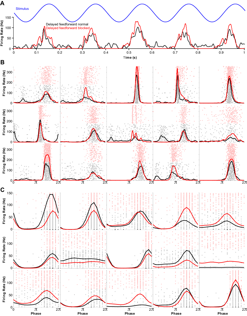
Figure 6: Responses of the 15 pyramidal cells in our data set. Parallel fiber input was intact (black) or blocked (red). A) One second excerpt of the responses to the 5 Hz AM stimulus (blue). Responses were converted to instantaneous firing rates (i.e. convolved with a 10 ms Gaussian) and averaged across the 15 cells of our data set. B) PSTH (cycle histogram) or responses of each cell to 5 Hz stimuli. Raster plots of spiking for each cycle are shown in the background. C) Same as B but with high frequency input (120 Hz).

Figure 7 shows the firing rate of the entire population of $N=1000$ (target) cells as a function of the chosen thresholds and synaptic variability parameters, for both low and high frequency stimuli. Each panel contains relevant correlation values $\varrho(q,\theta)$.

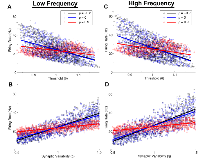
Figure 7: Resulting firing rate as a function of heterogeneous parameter values. A) Relationship between firing rate and threshold $\theta$ for all 1000 LIF neurons with representative correlation $\varrho(q,\theta)\in\{-0.2,0,0.9\}$ values for $\phi=5$ Hz. B) Relationship between firing rate and $q$ for all 1000 LIF neurons with representative correlation $\varrho$ values for $\phi=5$ Hz. C) and D) similar to A) and B) but with $\phi=120$ Hz input frequency. Although the firing rate is strongly related to the threshold, the synaptic variability has a weaker although positive correlation with the resulting firing rate.

References

- Abbott and van Vreeswijk (1993) Abbott LF, van Vreeswijk C (1993) Asynchronous States in Networks of Pulse-Coupled Oscillators. Physical Review E 48:1483–1490
- Ahn et al (2014) Ahn J, Kreeger L, Lubejko S, Butts D, MacLeod K (2014) Heterogeneity of intrinsic biophysical properties among cochlear nucleus neurons improves the population coding of temporal information. Journal of Neurophysiology 111(11):2320–2331
- Apfaltrer et al (2006) Apfaltrer F, Ly C, Tranchina D (2006) Population density methods for stochastic neurons with realistic synaptic kinetics: Firing rate dynamics and fast computational methods. Network: Computation in Neural Systems 17:373–418
- Averbeck et al (2006) Averbeck B, Latham P, Pouget A (2006) Neural correlations, population coding and computation. Nature Reviews Neuroscience 7:358–366
- Azouz and Gray (2000) Azouz R, Gray CM (2000) Dynamic spike threshold reveals a mechanism for synaptic coincidence detection in cortical neurons in vivo. Proceedings of the National Academy of Sciences 97(14):8110–8115
- Barna et al (1998) Barna G, Gröbler T, Érdi P (1998) Statistical model of the hippocampal CA3 region, ii. The population framework: model of rhythmic activity in CA3 slice. Biological Cybernetics 79:309–321
- Bastian (1986) Bastian J (1986) Gain control in the electrosensory system mediated by descending inputs to the electrosensory lateral line lobe. Journal of Neuroscience 6(2):553–562
- Bastian and Nguyenkim (2001) Bastian J, Nguyenkim J (2001) Dendritic modulation of burst-like firing in sensory neurons. Journal of Neurophysiology 85(1):10–22
- Bastian et al (2004) Bastian J, Chacron M, Maler L (2004) Plastic and nonplastic pyramidal cells perform unique roles in a network capable of adaptive redundancy reduction. Neuron 41(5):767–779
- Berman and Maler (1999) Berman N, Maler L (1999) Neural architecture of the electrosensory lateral line lobe: adaptations for coincidence detection, a sensory searchlight and frequency-dependent adaptive filtering. Journal of Experimental Biology 202(10):1243–1253
- Bol et al (2011) Bol K, Marsat G, Harvey-Girard E, Longtin A, Maler L (2011) Frequency-tuned cerebellar channels and burst-induced ltd lead to the cancellation of redundant sensory inputs. The Journal of Neuroscience 31(30):11,028–11,038
- Bremaud et al (2007) Bremaud A, West D, Thomson A (2007) Binomial parameters differ across neocortical layers and with different classes of connections in adult rat and cat neocortex. Proceedings of the National Academy of Sciences 104:14,134–14,139
- Brown et al (2004) Brown E, Moehlis J, Holmes P (2004) On the Phase Reduction and Response Dynamics of Neural Oscillator Populations. Neural Computation 16:673–715
- Brunel and Hakim (1999) Brunel N, Hakim V (1999) Fast global oscillations in networks of integrate-and-fire neurons with low firing rates. Neural Computation 11:1621–1671
- Brunel and Latham (2003) Brunel N, Latham P (2003) Firing Rate of the Noisy Quadratic Integrate-and-Fire neuron. Neural Computation 15:2281–2306
- Brunel et al (2001) Brunel N, Chance F, Fourcaud N, Abbott L (2001) Effects of Synaptic Noise and Filtering on the Frequency Response of Spiking Neurons. Physical Review Letters 86:2186–2189
- Bruno and Simons (2002) Bruno R, Simons D (2002) Feedforward mechanisms of excitatory and inhibitory cortical receptive fields. The Journal of Neuroscience 22(24):10,966–10,975
- Chacron et al (2005) Chacron M, Maler L, Bastian J (2005) Feedback and feedforward control of frequency tuning to naturalistic stimuli. The Journal of Neuroscience 25(23):5521–5532
- Chacron and Bastian (2008) Chacron MJ, Bastian J (2008) Population coding by electrosensory neurons. Journal of Neurophysiology 99(4):1825–1835
- Chelaru and Dragoi (2008) Chelaru M, Dragoi V (2008) Efficient coding in heterogeneous neuronal populations. Proceedings of the National Academy of Sciences 105:16,344–16,349
- Cohen and Kohn (2011) Cohen M, Kohn A (2011) Measuring and interpreting neuronal correlations. Nature Neuroscience 14:811–819
- Doiron et al (2001) Doiron B, Longtin A, Turner RW, Maler L (2001) Model of gamma frequency burst discharge generated by conditional backpropagation. Journal of neurophysiology 86(4):1523–1545
- Doiron et al (2003) Doiron B, Chacron MJ, Maler L, Longtin A, Bastian J (2003) Inhibitory feedback required for network oscillatory responses to communication but not prey stimuli. Nature 421(6922):539–543
- Doiron et al (2016) Doiron B, Litwin-Kumar A, Rosenbaum R, Ocker G, Josić K (2016) The mechanics of state-dependent neural correlations. Nature Neuroscience 19(3):383–393
- Ecker et al (2011) Ecker A, Berens P, Tolias A, Bethge M (2011) The effect of noise correlations in populations of diversely tuned neurons. The Journal of Neuroscience 31(40):14,272–14,283
- Faul et al (2007) Faul F, Erdfelder E, Lang AG, Buchner A (2007) G* power 3: A flexible statistical power analysis program for the social, behavioral, and biomedical sciences. Behavior research methods 39(2):175–191
- Faul et al (2009) Faul F, Erdfelder E, Buchner A, Lang AG (2009) Statistical power analyses using g* power 3.1: Tests for correlation and regression analyses. Behavior research methods 41(4):1149–1160
- Ferster and Miller (2000) Ferster D, Miller K (2000) Neural mechanisms of orientation selectivity in the visual cortex. Annual Review of Neuroscience 23(1):441–471
- Fourcaud and Brunel (2002) Fourcaud N, Brunel N (2002) Dynamics of the Firing Probability of Noisy Integrate-and-Fire Neuron. Neural Computation 14:2057–2110
- Frank and Becker (1964) Frank K, Becker M (1964) Microelectrodes for recording and stimulation. In: Nastuk W (ed) Physical techniques in biological research, New York: Academic Press, pp 23–84
- Georgopoulos et al (1986) Georgopoulos A, Schwartz A, Kettner R (1986) Neuronal population coding of movement direction. Science 233(4771):1416–1419
- Gerstner (2000) Gerstner W (2000) Population Dynamics of Spiking Neurons: Fast Transients, Asynchronous States, and Locking. Neural Computation 12:43–90
- Gussin et al (2007) Gussin D, Benda J, Maler L (2007) Limits of linear rate coding of dynamic stimuli by electroreceptor afferents. Journal of Neurophysiology 97(4):2917–2929
- Hermann and Touboul (2012) Hermann G, Touboul J (2012) Heterogeneous connections induce oscillations in large-scale networks. Physical Review Letters 109:018,702
- Hertäg et al (2014) Hertäg L, Durstewitz D, Brunel N (2014) Analytical approximations of the firing rate of an adaptive exponential integrate-and-fire neuron in the presence of synaptic noise. Frontiers in computational neuroscience 8
- Hoenig and Heisey (2001) Hoenig JM, Heisey DM (2001) The abuse of power: the pervasive fallacy of power calculations for data analysis. The American Statistician 55(1):19–24
- Huertas and Smith (2006) Huertas MA, Smith GD (2006) A multivariate population density model of the dLGN/PGN relay. Journal of Computational Neuroscience 21:ISSN: 929–5313 (Paper), 1573–6873 (Online). DOI: 10.1007/s10,827–006–7753–2
- Hunsberger et al (2014) Hunsberger E, Scott M, Eliasmith C (2014) The competing benefits of noise and heterogeneity in neural coding. Neural computation 26(8):1600–1623
- Josić et al (2009) Josić K, Shea-Brown E, Doiron B, de la Rocha J (2009) Stimulus-dependent correlations and population codes. Neural Computation 21:2774–2804
- Kay (1993) Kay S (1993) Fundamentals of Statistical Signal Processing, Volume 1: Estimation Theory. Prentice Hall PTR
- Knight (1972) Knight BW (1972) The relationship between the firing rate of a single neuron and the level of activity in a population of neurons. Experimental evidence for resonant enhancement in the population response. Journal of General Physiology 59:767–778
- Litwin-Kumar et al (2012) Litwin-Kumar A, Chacron M, Doiron B (2012) The spatial structure of stimuli shapes the timescale of correlations in population spiking activity. PLoS Computational Biology 8(9):e1002,667
- Ly (2015) Ly C (2015) Firing rate dynamics in recurrent spiking neural networks with intrinsic and network heterogeneity. Journal of Computational Neuroscience 39:311–327
- Ly and Ermentrout (2010) Ly C, Ermentrout B (2010) Analysis of recurrent networks of pulse-coupled noisy neural oscillators. SIAM Journal on Applied Dynamical Systems 9:113–137
- Ly and Tranchina (2007) Ly C, Tranchina D (2007) Critical Analysis of Dimension Reduction by a Moment Closure Method in a Population Density Approach to Neural Network Modeling. Neural Computation 19:2032–2092
- Ly et al (2012) Ly C, Middleton J, Doiron B (2012) Cellular and circuit mechanisms maintain low spike co-variability and enhance population coding in somatosensory cortex. Frontiers in Computational Neuroscience 6:1–26, DOI 10.3389/fncom.2012.00007
- Maler (2007) Maler L (2007) Neural strategies for optimal processing of sensory signals. Progress in Brain Research 165:135–154
- Maler (2009) Maler L (2009) Receptive field organization across multiple electrosensory maps. i. columnar organization and estimation of receptive field size. Journal of Comparative Neurology 516(5):376–393
- Maler et al (1991) Maler L, Sas E, Johnston S, Ellis W (1991) An atlas of the brain of the electric fish apteronotus leptorhynchus. Journal of chemical neuroanatomy 4(1):1–38
- Marder and Goaillard (2006) Marder E, Goaillard J (2006) Variability, compensation and homeostasis in neuron and network function. Nature Reviews Neuroscience 7:563–574
- Marsat and Maler (2012) Marsat G, Maler (2012) Preparing for the unpredictable: adaptive feedback enhances the response to unexpected communication signals. Journal of Neurophysiology 107(4):1241–1246
- Marsat and Maler (2010) Marsat G, Maler L (2010) Neural heterogeneity and efficient population codes for communication signals. Journal of Neurophysiology 104:2543–2555
- Marsat et al (2012) Marsat G, Longtin A, Maler L (2012) Cellular and circuit properties supporting different sensory coding strategies in electric fish and other systems. Current Opinion in Neurobiology 22(4):686–692
- Marsat et al (2014) Marsat G, Hupé GJ, Allen K (2014) Heterogeneous response properties in a population of sensory neurons are structured to efficiently code naturalistic stimuli. Neuroscience Meeting Planner, Program # (181.20)
- Mehaffey et al (2008) Mehaffey W, Maler L, Turner R (2008) Intrinsic frequency tuning in ell pyramidal cells varies across electrosensory maps. Journal of Neurophysiology 99(5):2641–2655
- Mejias and Longtin (2012) Mejias J, Longtin A (2012) Optimal heterogeneity for coding in spiking neural networks. Physical Review Letters 108:228,102
- Mejias and Longtin (2014) Mejias J, Longtin A (2014) Differential effects of excitatory and inhibitory heterogeneity on the gain and asynchronous state of sparse cortical networks. Frontiers in computational neuroscience 8
- Mejias et al (2013) Mejias J, Marsat G, Bol K, Maler L, Longtin A (2013) Learning contrast-invariant cancellation of redundant signals in neural systems. PLoS computational biology 9(9):e1003,180
- Middleton et al (2009) Middleton J, Longtin A, Benda J, Maler L (2009) Postsynaptic receptive field size and spike threshold determine encoding of high-frequency information via sensitivity to synchronous presynaptic activity. Journal of Neurophysiology 101(3):1160–1170
- Moreno-Bote and Parga (2006) Moreno-Bote R, Parga N (2006) Auto- and Crosscorrelograms for the Spike Response of Leaky Integrate-and-Fire Neurons with Slow Synapses. Physical Review Letters 96:028,101
- Nesse et al (2008) Nesse WH, Borisyuk A, Bressloff P (2008) Fluctuation-driven rhythmogenesis in an excitatory neuronal network with slow adaptation. Journal of Computational Neuroscience 25:317–333
- Nicola et al (2015) Nicola W, Ly C, Campbell SA (2015) One-dimensional population density approaches to recurrently coupled networks of neurons with noise. SIAM Journal on Applied Mathematics (in press):–
- Noonan et al (2003) Noonan L, Doiron B, Laing C, Longtin A, Turner R (2003) A dynamic dendritic refractory period regulates burst discharge in the electrosensory lobe of weakly electric fish. The Journal of neuroscience 23(4):1524–1534
- Nykamp and Tranchina (2000) Nykamp D, Tranchina D (2000) A Population Density Approach That Facilitates Large-Scale Modeling of Neural Networks: Analysis and an Application to Orientation Tuning. Journal of Computational Neuroscience 8:19–50
- Omurtag et al (2000) Omurtag A, Knight BW, Sirovich L (2000) On the Simulation of Large Populations of Neurons. Journal of Computational Neuroscience 8:51–63
- Oswald et al (2009) Oswald A, Doiron B, Rinzel J, Reyes A (2009) Spatial profile and differential recruitment of gabab modulate oscillatory activity in auditory cortex. The Journal of Neuroscience 29:10,321–10,334
- Padmanabhan and Urban (2010) Padmanabhan K, Urban N (2010) Intrinsic biophysical diversity decorrelates neuronal firing while increasing information content. Nature Neuroscience 13:1276–1282
- Parker (2003) Parker D (2003) Variable properties in a single class of excitatory spinal synapse. The Journal of neuroscience 23(8):3154–3163
- Pouille and Scanziani (2001) Pouille F, Scanziani M (2001) Enforcement of temporal fidelity in pyramidal cells by somatic feed-forward inhibition. Science 293(5532):1159–1163
- Priebe and Ferster (2008) Priebe N, Ferster D (2008) Inhibition, spike threshold, and stimulus selectivity in primary visual cortex. Neuron 57(4):482–497
- Richardson (2007) Richardson M (2007) Firing-rate response of linear and nonlinear integrate-and-fire neurons to modulated current-based and conductance-based synaptic drive. Physical Review E 76:021,919
- Richardson (2008) Richardson M (2008) Spike-train spectra and network response functions for non-linear integrate-and-fire neurons. Biological Cybernetics 99:381–392
- Saunders and Bastian (1984) Saunders J, Bastian J (1984) The physiology and morphology of two types of electrosensory neurons in the weakly electric fish apteronotus leptorhynchus. Journal of Comparative Physiology A 154(2):199–209
- Shamir and Sompolinsky (2006) Shamir M, Sompolinsky H (2006) Implications of neuronal diversity on population coding. Neural Computation 18:1951–1986
- Simmonds and Chacron (2015) Simmonds B, Chacron MJ (2015) Activation of parallel fiber feedback by spatially diffuse stimuli reduces signal and noise correlations via independent mechanisms in a cerebellum-like structure. PLOS Computational Biology 11(1):e1004,034
- Thomas (1997) Thomas L (1997) Retrospective power analysis. Conservation Biology 11(1):276–280
- Tranchina (2009) Tranchina D (2009) Population density methods in large-scale neural network modelling. In: Laing C, Lord G (eds) Stochastic Methods in Neuroscience, Oxford University Press, chap 7
- Tripathy et al (2013) Tripathy S, Padmanabhan K, Gerkin R, Urban N (2013) Intermediate intrinsic diversity enhances neural population coding. Proceedings of the National Academy of Sciences 110:8248–8253
- Wilbur and Rinzel (1982) Wilbur W, Rinzel J (1982) An analysis of Stein’s model for stochastic neural excitation. Biological cybernetics 45:107–114
- Xue et al (2014) Xue M, Atallah BV, Scanziani M (2014) Equalizing excitation-inhibition ratios across visual cortical neurons. Nature 511:596–600