The scalar-scalar-tensor inflationary three-point function in the axion monodromy model

Abstract

The axion monodromy model involves a canonical scalar field that is governed by a linear potential with superimposed modulations. The modulations in the potential are responsible for a resonant behavior which gives rise to persisting oscillations in the scalar and, to a smaller extent, in the tensor power spectra. Interestingly, such spectra have been shown to lead to an improved fit to the cosmological data than the more conventional, nearly scale invariant, primordial power spectra. The scalar bi-spectrum in the model too exhibits continued modulations and the resonance is known to boost the amplitude of the scalar non-Gaussianity parameter to rather large values. An analytical expression for the scalar bi-spectrum had been arrived at earlier which, in fact, has been used to compare the model with the cosmic microwave background anisotropies at the level of three-point functions involving scalars. In this work, with future applications in mind, we arrive at a similar analytical template for the scalar-scalar-tensor cross-correlation. We also analytically establish the consistency relation (in the squeezed limit) for this three-point function. We conclude with a summary of the main results obtained.

1 Introduction

Until very recently, inflationary models were compared with the data at the level of two-point functions, i.e. the inflationary scalar and tensor power spectra were compared with the angular power spectra of the Cosmic Microwave Background (CMB) and the matter power spectrum associated with the Large Scale Structure (LSS) [1, 2, 3, 4, 5, 6, 7, 8, 9]. Over the last decade and a half, it has been realized that non-Gaussianities in general and the three-point functions in particular can provide strong constraints on the physics of the early universe. On one hand, there has been tremendous progress in understanding the generation of non-Gaussianities during inflation [10, 11, 12, 13, 14, 15, 16, 17, 18, 19, 20, 21, 22] and the corresponding signatures on the CMB and the LSS [23, 24, 25, 26, 27, 28, 29, 30, 31, 32, 33, 34, 35, 36, 37, 38, 39]. On the other hand, the expectation alluded to above has been largely corroborated by the strong constraints that have been arrived at from the Planck CMB data on the scalar non-Gaussianity parameter $f_{{}_{\rm NL}}$ [40]. The recent observations seem to suggest that the primordial perturbations are consistent with a Gaussian distribution.

A nearly scale invariant primordial scalar power spectrum is remarkably consistent with the observations of the CMB [1, 2, 3, 5, 6, 7, 4, 8, 9]. However, it has been repeatedly noticed that certain features in the inflationary power spectrum can improve the fit to the data (for instance, see Refs. [41, 42, 43, 44, 45, 46, 47, 48, 49]). One such type of feature is continued oscillations in the scalar power spectrum that extends over a wide range of scales [50, 51, 52, 53, 54, 55, 56, 57]. Such a power spectrum is known to be generated by the so-called axion monodromy model, motivated by string theory [58, 59, 60, 61, 62]. The model is described by a linear potential with superimposed oscillations. The oscillations in the potential give rise to a resonant behavior which leads to continued modulations in the scalar and tensor power spectra. At the cost of two or three extra parameters, the resulting power spectra are known to improve the fit to the CMB data from the Wilkinson Microwave Anisotropy Probe (WMAP) and Planck by as much as $\Delta\chi^{2}\simeq 10$–$20$ [59, 60, 61, 56, 57]. Ideally, one would like to carry out a similar analysis of comparing the model with the CMB data at the level of the three-point functions as well. But, it proves to be numerically taxing to evaluate the three-point functions in these models (see, for instance, Ref. [63]). In such a situation, clearly, it will be convenient if there exist analytical templates for the inflationary three-point functions. Such a template for the scalar bi-spectrum has been arrived at earlier [58, 64], which has been utilized towards comparing models leading to oscillatory features with the CMB data [65, 66].

Apart from the scalar bi-spectrum, there exist three other three-point functions which involve the tensor perturbations [14]. Amongst these three-point functions, the scalar-scalar-tensor cross-correlation has the largest amplitude after the scalar bi-spectrum (in this context, see Refs. [14, 67, 68, 69, 70, 71, 72, 73, 74]). In this work, motivated by the efforts towards arriving at an analytical template for the scalar bi-spectrum in the axion monodromy model, we obtain a similar template for the scalar-scalar-tensor three-point function for an arbitrary triangular configuration of the wavevectors. In the case of the scalar bi-spectrum, in order to determine the dominant contribution due to the oscillations in the potential, it was sufficient to take into account the effects due to the changes in the behavior of the slow roll parameters, and one could work with the simple de Sitter modes for the curvature perturbation. In contrast, to evaluate the scalar-scalar-tensor cross correlation, we find that apart from the changes in the behavior of the slow roll parameters, we also need to take into account the modifications to the de Sitter modes. As in the purely scalar case [75, 76, 77, 78, 79, 80, 81, 82, 83, 84], the other three-point functions involving the tensors are also known to satisfy the so-called consistency relation in the squeezed limit [68, 70, 85, 71, 86, 87]. We shall analytically establish the consistency condition for the scalar-scalar-tensor three-point function in the axion monodromy model.

The remainder of this paper is organized as follows. In the next section, we shall briefly discuss the important aspects of the axion monodromy model and arrive at the scalar and tensor power spectra in the model. In Sec. 3, we shall gather the essential expressions describing the scalar-scalar-tensor three-point function and the corresponding non-Gaussianity parameter. In Sec. 4, we shall arrive at an analytical expression for the scalar-scalar-tensor cross-correlation under certain approximations. To illustrate the extent of accuracy of the approximations, we shall also compare the analytical result with the corresponding numerical result. Further, in Sec. 5, we shall analytically verify the consistency relation for the three-point function in the squeezed limit. We shall conclude in Sec. 6 with a brief summary of the results obtained.

A few remarks on our conventions and notations seem essential at this stage of our discussion. We shall work with natural units wherein $\hbar=c=1$, and define the Planck mass to be $M_{{}_{\rm Pl}}=(8\,\pi\,G)^{-1/2}$. We shall adopt the signature of the metric to be $(-,+,+,+)$. We shall assume the background to be the spatially flat Friedmann-Lemaître-Robertson-Walker (FLRW) line element that is described by the scale factor $a$ and the Hubble parameter $H$. As is convenient, we shall switch between various parameterizations of time, viz. the cosmic time $t$, the conformal time $\eta$ or e-folds denoted by $N$. An overdot and an overprime shall represent differentiation with respect to the cosmic and the conformal time coordinates, respectively. We shall restrict our attention in this work to inflationary models involving the canonical scalar field. Note that, in such a case, the first and second slow roll parameters are defined as $\epsilon_{1}=-\dot{H}/H^{2}$ and $\epsilon_{2}={\rm d}\ln\,\epsilon_{1}/{\rm d}N$.

2 The axion monodromy model

In this section, we shall summarize the essential aspects of the axion monodromy model. We shall discuss the evolution of the background as well as the evolution of the scalar and tensor perturbations and also arrive at the corresponding power spectra.

2.1 The evolution of the background and the slow roll parameters

The axion monodromy model is described by a linear potential with superimposed oscillations [59, 58, 60, 61]. The potential is given by

$$V(\phi)=\mu^{3}\,\phi+\mu^{3}\,b\,f\,{\rm cos}\,\left(\frac{\phi}{f}\right),$$ (2.1)

where $b$ is a dimensionless quantity and we have ignored a possible phase factor in the trigonometric function. Throughout this work, we shall assume that $b$ is small and attempt to derive all the results at the linear order in $b$ (as we shall discuss in due course, the constraint from the recent Planck data suggests that $b$ is indeed small, of the order of $10^{-2}$). Evidently, this assumption is equivalent to considering the trigonometric modulations as small departures from the linear potential. We shall also assume that the linear potential admits slow roll and that the modulations lead to deviations from the monotonic slow roll behavior [58].

The equation of motion governing the scalar field described by the potential (2.1) above is given by

$${\ddot{\phi}}+3\,H\,{\dot{\phi}}+\mu^{3}-\mu^{3}\,b\,{\rm sin}\left(\frac{\phi}{f}\right)=0,$$ (2.2)

with the Hubble parameter $H={\dot{a}}/a$ being determined by the first Friedmann equation, viz. 

$$H^{2}=\frac{1}{3\,M_{{}_{\rm Pl}}^{2}}\left[\frac{\dot{\phi}^{2}}{2}+V(\phi)\right].$$ (2.3)

Since we shall assume that $b$ is small, we can write the background inflaton as a slowly rolling part plus a part which describes the modulations as

$$\phi=\phi_{0}+b\,\phi_{1}+\ldots.$$ (2.4)

As we mentioned, we shall limit ourselves to terms which are linear in $b$. At the leading order, under the slow roll approximation, the equations (2.2) and (2.3) simplify to

$$3\,H\,{\dot{\phi}}_{0} \simeq -\mu^{3},$$ (2.5a)

$$3\,H^{2}\,M_{{}_{\rm Pl}}^{2} \simeq \mu^{3}\,\phi_{0}.$$ (2.5b)

These equations can be easily integrated to yield the leading order term in the inflaton to be

$$\phi_{0}(t)=\left[\phi_{\ast}^{3/2}-\frac{\sqrt{3\,\mu^{3}}}{2}\,M_{{}_{\rm Pl}}\,\left(t-t_{\ast}\right)\right]^{2/3},$$ (2.6)

where $\phi_{0}(t_{\ast})=\phi_{\ast}$, with $t_{\ast}$ denoting the time when the pivot scale, say, $k_{\ast}$, leaves the Hubble radius. It should be noted that, in order to achieve about $60$–$70$ e-folds of inflation, we shall require that $\phi_{\ast}\simeq 10\,M_{{}_{\rm Pl}}$.

Let us now consider the behavior of $\phi_{1}$. The differential equation satisfied by the component $\phi_{1}$ can be obtained to be

$${\ddot{\phi}}_{1}+\frac{\sqrt{3\,\mu^{3}\,\phi_{0}}}{M_{{}_{\rm Pl}}}\,{\dot{\phi}}_{1}-\frac{\mu^{3}}{2\,\phi_{0}}\,\phi_{1}=\mu^{3}\,{\rm sin}\left(\frac{\phi_{0}}{f}\right),$$ (2.7)

where we have made use of the fact that, until the first order in $b$, under the slow roll approximation, we can write

$$H^{2}\simeq\frac{\mu^{3}}{3\,M_{{}_{\rm Pl}}^{2}}\,\left(\phi_{0}+b\,\phi_{1}\right).$$ (2.8)

If we make use of the solution (2.6) for $\phi_{0}$, the above equation governing $\phi_{1}$ can be expressed as

$$\frac{{\rm d}^{2}\phi_{1}}{{\rm d}\phi_{0}^{2}}-\frac{3\,\phi_{0}}{M_{{}_{\rm Pl}}^{2}}\,\frac{{\rm d}\phi_{1}}{{\rm d}\phi_{0}}-\frac{3\,\phi_{1}}{2\,M_{{}_{\rm Pl}}^{2}}=\frac{3\,\phi_{0}}{M_{{}_{\rm Pl}}^{2}}\,{\rm sin}\left(\frac{\phi_{0}}{f}\right).$$ (2.9)

This equation can be integrated to arrive at the following solution for $\phi_{1}$:

$$\phi_{1}(\phi_{0})=\frac{3\,f^{2}\,\phi_{\ast}/M_{{}_{\rm Pl}}^{2}}{1+(3\,f\,\phi_{\ast}/M_{{}_{\rm Pl}}^{2})^{2}}\,\left[-{\rm sin}\left(\frac{\phi_{0}}{f}\right)+\frac{3\,f\,\phi_{\ast}}{M_{{}_{\rm Pl}}^{2}}\,{\rm cos}\left(\frac{\phi_{0}}{f}\right)\right],$$ (2.10)

which can be written as

$$\phi_{1}(\phi_{0})=-\frac{3\,f^{2}\,\phi_{\ast}/M_{{}_{\rm Pl}}^{2}}{\left[1+(3\,f\,\phi_{\ast}/M_{{}_{\rm Pl}}^{2})^{2}\right]^{1/2}}\,{\rm sin}\left(\frac{\phi_{0}}{f}-\psi_{1}\right),$$ (2.11)

where

$${\rm sin}\,\psi_{1}=\frac{3\,f\,\phi_{\ast}/M_{{}_{\rm Pl}}^{2}}{\left[1+(3\,f\,\phi_{\ast}/M_{{}_{\rm Pl}}^{2})^{2}\right]^{1/2}}\;.$$ (2.12)

Note that, when $f\,\phi_{\ast}/M_{{}_{\rm Pl}}^{2}$ is assumed to be small (as we shall discuss later, the constraints from the recent CMB observations suggest that $f\,\phi_{\ast}/M_{{}_{\rm Pl}}^{2}\simeq 7.6346\times 10^{-2}$), we can write

$$\phi_{1}(\phi_{0})=-\frac{3\,f^{2}\,\phi_{\ast}}{M_{{}_{\rm Pl}}^{2}}\,{\rm sin}\left(\frac{\phi_{0}}{f}\right).$$ (2.13)

Having understood the behavior of the background inflaton, let us now evaluate the first and the second slow roll parameters. Recall that the first slow roll parameter is given by $\epsilon_{1}=-{\dot{H}}/H^{2}={\dot{\phi}}^{2}/(2\,H^{2}\,M_{{}_{\rm Pl}}^{2})$. Let us write the first slow roll parameter as $\epsilon_{1}=\epsilon_{1}^{0}+\epsilon_{1}^{\rm c}$, where $\epsilon_{1}^{0}$ is the contribution due to $\phi_{0}$, while $\epsilon_{1}^{\rm c}$ is the correction at the first order in $b$. As one would expect, $\epsilon_{1}^{0}$ will roughly be constant and will be of the order of $\epsilon_{1}^{0}=\epsilon_{1}^{\ast}\simeq M_{{}_{\rm Pl}}^{2}/(2\,\phi_{\ast}^{2})$, determined by the linear term in the potential. Upon making use of the solutions we have obtained above, we can show that, the quantity $\epsilon_{1}^{\rm c}$ is given by

$$\epsilon_{1}^{\rm c}=-\frac{3\,b\,f}{\phi_{\ast}}\cos\left(\frac{\phi_{0}}{f}\right).$$ (2.14)

In arriving at this expression, we have again made the assumption that $f\,\phi_{\ast}/M_{{}_{\rm Pl}}^{2}\ll 1$. The second slow roll parameter can be expressed as $\epsilon_{2}={\dot{\epsilon}}_{1}/(H\,\epsilon_{1})$. One can show that $\epsilon_{2}=2\,(\delta+\epsilon_{1})$, where $\delta={\ddot{H}}/(H\,{\dot{H}})={\ddot{\phi}}/(H\,{\dot{\phi}})$. If we write $\delta=\delta_{0}+\delta_{1}$, where $\delta_{0}$ corresponds to the case wherein $b$ vanishes, then we can show that $\delta_{0}=\epsilon_{1}^{\ast}$ and $\epsilon_{2}^{*}=4\,\epsilon_{1}^{\ast}$. Also, for small $f\,\phi_{\ast}/M_{{}_{\rm Pl}}^{2}$, we find that $\delta_{1}$ can be expressed as

$$\delta_{1}=-3\,b\,\sin\left(\frac{\phi_{0}}{f}\right).$$ (2.15)

2.2 The evolution of the perturbations and the power spectra

The assumptions and approximations that we have made in the previous sub-section enable us to analytically explore the evolution of perturbations and calculation of the power spectra [58].

Let us begin by summarizing a few basic points concerning the scalar power spectrum. Recall that, upon quantization, the curvature perturbation ${\mathcal{R}}$ can be decomposed in terms of the corresponding Fourier modes as follows:

$$\hat{{\mathcal{R}}}(\eta,{\bf x})=\int\frac{{\rm d}^{3}{\bm{k}}}{\left(2\,\pi\right)^{3/2}}\,\hat{{\mathcal{R}}}_{\bm{k}}(\eta)\,{\rm e}^{i\,{\bm{k}}\cdot{\bm{x}}}=\int\frac{{\rm d}^{3}{\bm{k}}}{\left(2\,\pi\right)^{3/2}}\,\left(\hat{a}_{\bm{k}}\,f_{k}(\eta)\,{\rm e}^{i\,{\bm{k}}\cdot{\bm{x}}}+\hat{a}^{\dagger}_{\bf k}\,f^{*}_{k}(\eta)\,{\rm e}^{-i\,{\bm{k}}\cdot{\bm{x}}}\right),\\$$ (2.16)

where the modes $f_{k}$ satisfy the differential equation

$$f_{k}^{\prime\prime}+2\,\frac{z^{\prime}}{z}\,f_{k}^{\prime}+k^{2}\,f_{k}=0,\\$$ (2.17)

with $z=\sqrt{2\,\epsilon_{1}}\,a\,M_{{}_{\rm Pl}}$, while the annihilation and the creation operators ${\hat{a}}_{\bm{k}}$ and $\hat{a}^{\dagger}_{\bm{k}}$ obey the standard commutation relations. The scalar power spectrum, viz.  ${\mathcal{P}}_{{}_{\rm S}}(k)$, is defined as

$$\langle\,{\hat{\mathcal{R}}}_{\bm{k}}(\eta)\,{\hat{\mathcal{R}}}_{\bm{k}^{\prime}}(\eta)\,\rangle=\frac{(2\,\pi)^{2}}{2\,k^{3}}\,{\mathcal{P}}_{{}_{\rm S}}(k)\;\delta^{(3)}({\bm{k}}+{\bm{k}^{\prime}}),\\$$ (2.18)

where the expectation value on the left hand side is to be evaluated in the specified initial quantum state of the perturbations. If one assumes the initial state of the perturbations to be the vacuum state $|0\rangle$ (defined as ${\hat{a}}_{\bm{k}}|0\rangle=0$ $\forall\,{\bm{k}}$) then, on making use of the decomposition (2.16) in the above definition, the inflationary scalar power spectrum ${\mathcal{P}}_{{}_{\rm S}}(k)$ can be expressed as

$${\mathcal{P}}_{{}_{\rm S}}(k)=\frac{k^{3}}{2\,\pi^{2}}\,|f_{k}|^{2}.$$ (2.19)

The amplitude $|f_{k}|$ on the right hand side of the above expression is to be evaluated when the modes are sufficiently outside the Hubble radius. It is useful to note here that the scalar spectral index $n_{{}_{\rm S}}$ is defined as

$$n_{{}_{\rm S}}=1+\frac{{\rm d}\ln{\mathcal{P}}_{{}_{\rm S}}(k)}{{\rm d}\ln k}.\\$$ (2.20)

Let us analytically evaluate the scalar power spectrum in the axion monodromy model [58]. If we choose to work in terms of the new variable $x=-k\,\eta$ and use the exact relation

$$\frac{z^{\prime}}{z}=a\,H\,\left(1+\epsilon_{1}+\delta\right),$$ (2.21)

we can rewrite the differential equation (2.17) governing the mode $f_{k}$ as

$$\frac{{\rm d}^{2}f_{k}}{{\rm d}x^{2}}+2\,\left(1+\epsilon_{1}+\delta\right)\,\left(\frac{a\,H}{-k}\right)\,\frac{{\rm d}f_{k}}{{\rm d}x}+f_{k}=0.$$ (2.22)

At the leading order in slow roll, we have

$$a\,H\simeq-\frac{1+\epsilon_{1}}{\eta}.$$ (2.23)

We shall work in the de Sitter approximation when $b=0$, which corresponds to ignoring the contributions due to the $\epsilon_{1}^{\ast}$ term. The effects due to the $\delta_{1}$ term dominate the effects due to the $\epsilon_{1}^{\rm c}$ term. Under these conditions, we can write the above differential equation describing $f_{k}$ as follows:

$$\frac{{\rm d}^{2}f_{k}}{{\rm d}x^{2}}-\frac{2\,\left(1+\delta_{1}\right)}{x}\,\frac{{\rm d}f_{k}}{{\rm d}x}+f_{k}=0.$$ (2.24)

In the slow roll limit determined by the linear potential wherein $\delta_{1}$ can be ignored, the positive frequency modes satisfying the above differential equation can be written in the de Sitter form as

$$f_{k}^{+}(x)=i\,f_{k}^{0}\,\left(1-i\,x\right)\,{\rm e}^{i\,x},$$ (2.25)

where $f_{k}^{0}=H_{0}/(2\,M_{{}_{\rm Pl}}\,\sqrt{k^{3}\,\epsilon_{1}^{\ast}})$, with $H_{0}$ being given by $H_{0}^{2}=\mu^{3}\,\phi_{\ast}/(3\,M_{{}_{\rm Pl}}^{2})$. Hence, in the presence of a non-zero $\delta_{1}$, let us write the modes describing the curvature perturbation as [58]

$$f_{k}(x)=f_{k}^{+}(x)+c_{k}(x)\,f_{k}^{-}(x),$$ (2.26)

where $f_{k}^{-}(x)$ are the negative frequency modes that are related to the positive frequency modes by the relation $f_{k}^{-}(x)=f_{k}^{+\ast}(x)$. Note that the non-vanishing $\delta_{1}$ modifies the standard de Sitter modes $f_{k}^{+}(x)$. The non-trivial evolution of the modes is captured by the function $c_{k}(x)$.

The de Sitter modes $f_{k}^{\pm}$ satisfy the differential equation

$$\frac{{\rm d}^{2}f_{k}^{\pm}}{{\rm d}x^{2}}-\frac{2}{x}\,\frac{{\rm d}f_{k}^{\pm}}{{\rm d}x}+f_{k}^{\pm}=0.$$ (2.27)

Therefore, upon substituting the expression (2.26) in the differential equation (2.24), we obtain the following equation governing $c_{k}$:

$$\frac{{\rm d}}{{\rm d}x}\left[\left(1-\frac{i}{x}\right)\,{\rm e}^{-2\,i\,x}\,\frac{{\rm d}c_{k}}{{\rm d}x}\right]+\frac{i}{x^{2}}\,{\rm e}^{-2\,i\,x}\,\frac{{\rm d}c_{k}}{{\rm d}x}=\frac{2\,i\,\delta_{1}}{x}.$$ (2.28)

As is well known, the perturbations oscillate when they are well inside the Hubble radius. In this sub-Hubble regime, the oscillations in the perturbations resonate with the oscillations in the background quantities. This resonance occurs when $x\simeq M_{{}_{\rm Pl}}^{2}/(2\,f\,\phi_{\ast})$, which proves to be a large quantity for the parameter ranges of our interest (recall that, we had assumed $f\,\phi_{\ast}/M_{{}_{\rm Pl}}^{2}$ to be small). Therefore, the terms involving inverse powers of $x$ on the left hand side of the above differential equation can be ignored in the sub-Hubble regime and, under these conditions, the equation can be easily integrated. We find that the resulting $c_{k}(x)$ can be expressed as

$$c_{k}(x) = -\frac{3\,b\,f\,\phi_{\ast}}{2\,M_{{}_{\rm Pl}}^{2}}\,\biggl{[}{\rm e}^{i\,(\alpha_{1}+\phi_{k}/f)}\,{\rm e}^{-\pi\,M_{{}_{\rm Pl}}^{2}/(2\,f\,\phi_{\ast})}\;\Gamma\left(1+\frac{i\,M_{{}_{\rm Pl}}^{2}}{f\,\phi_{\ast}},-2\,i\,x\right)$$ (2.29)

$$+\,{\rm e}^{-i\,(\alpha_{1}+\phi_{k}/f)}\,{\rm e}^{\pi\,M_{{}_{\rm Pl}}^{2}/(2\,f\,\phi_{\ast})}\;\Gamma\left(1-\frac{i\,M_{{}_{\rm Pl}}^{2}}{f\,\phi_{\ast}},-2\,i\,x\right)\biggr{]},$$

where $\Gamma(a,x)$ is the incomplete Gamma function [88] and $\alpha_{1}=-X_{\rm res}\,{\rm ln}\,2$, with $X_{\rm res}=M_{{}_{\rm Pl}}^{2}/(f\,\phi_{\ast})$. Note that $X_{\rm res}$ is a large quantity since we have assumed $f\,\phi_{\ast}/M_{{}_{\rm Pl}}^{2}$ to be small. Note that, in arriving at the above expression, we have expressed $\phi_{0}$ in terms of $x$ as

$$\phi_{0}=\phi_{k}\,+\,\sqrt{2\,\epsilon_{1}^{*}}\,M_{{}_{\rm Pl}}\,{\rm ln}\,x,$$ (2.30)

where the quantity $\phi_{k}$ is given by

$$\phi_{k}=\phi_{\ast}-\sqrt{2\,\epsilon_{1}^{\ast}}\,M_{{}_{\rm Pl}}\,{\rm ln}\left(\frac{k}{k_{\ast}}\right)$$ (2.31)

with $k_{\ast}$ denoting the pivot scale. Since we have assumed that $f\,\phi_{\ast}/M_{{}_{\rm Pl}}^{2}\ll 1$, the first term in Eq. (2.29) is exponentially suppressed and hence can be ignored. Thus, we can express $c_{k}$ as

$$c_{k}(x)=-\frac{3\,b\,f\,\phi_{\ast}}{2\,M_{{}_{\rm Pl}}^{2}}\,{\rm e}^{-i\,\left(\phi_{k}/f+\alpha_{1}\right)}\,{\rm e}^{\pi\,M_{{}_{\rm Pl}}^{2}/2\,f\,\phi_{\ast}\,}\,\Gamma\left(1-\frac{i\,M_{{}_{\rm Pl}}^{2}}{f\,\phi_{\ast}},-2\,i\,x\right).$$ (2.32)

Note that, in deriving the above solution for $c_{k}(x)$, we had ignored inverse powers of $x$ on the left hand side of Eq. (2.28). We should emphasize here that this approximation is strictly valid only at sub-Hubble scales. However, since the complete mode approaches a constant value at late times, one finds that the largest contribution to the three-point functions arises from the sub-Hubble domain [58]. Hence, the above solution for $c_{k}(x)$ proves to be sufficient for evaluating the three-point function of our interest analytically. As we shall see, these arguments are corroborated by the numerical results we obtain.

The scalar power spectrum can now be obtained from the late time limit (i.e.  as $x\to 0$) of the modes $f_{k}$. We find that

$$c_{k}(0)=\frac{3\,i\,b\,\sqrt{\pi}}{\sqrt{2\,X_{\rm res}}}\,{\rm e}^{-i\,\left(\phi_{k}/f+\beta_{1}\right)},$$ (2.33)

where the phase $\beta_{1}=X_{\rm res}\,{\rm ln}\,X_{\rm res}-X_{\rm res}-X_{\rm res}\,{\rm ln}\,2-\pi/4$. Upon using this result, at the order $b$, we can express the scalar power spectrum as [58]

$${\mathcal{P}}_{{}_{\rm S}}(k)={\mathcal{P}}_{{}_{\rm S}}^{0}\,\left[1-c_{k}(0)-c_{k}^{\ast}(0)\right]={\mathcal{P}}_{{}_{\rm S}}^{0}\,\left[1-\delta n_{{}_{\rm S}}\,\sin\left(\frac{\phi_{k}}{f}+\beta_{1}\right)\right],$$ (2.34)

where ${\mathcal{P}}_{{}_{\rm S}}^{0}$ represents the amplitude of the scalar power spectrum which arises in the slow roll scenario when the oscillations in the potential are absent and the quantity $\phi_{k}$ depends on the wavenumber through the relation (2.31). The quantity ${\mathcal{P}}_{{}_{\rm S}}^{0}$ is given by

$${\mathcal{P}}_{{}_{\rm S}}^{0}=\frac{H_{0}^{2}}{8\,\pi^{2}\,M_{{}_{\rm Pl}}^{2}\,\epsilon_{1}^{\ast}}$$ (2.35)

and, for small $f\,\phi_{\ast}/M_{{}_{\rm Pl}}^{2}$, the quantity $\delta n_{{}_{\rm S}}$ can be expressed as

$$\delta n_{{}_{\rm S}}=\frac{3\,b\,\sqrt{2\pi}}{\sqrt{X_{\rm res}}}.$$ (2.36)

The sinusoidal term in the power spectrum leads to oscillations that extends over a wide range of scales. These oscillations result in continued modulations in the scalar spectral index $n_{{}_{\rm S}}$ [cf. Eq . (2.20)], which can be obtained from the expression (2.34) for the scalar power spectrum. In order to separate the contributions at the zeroth and first order in $b$, it is convenient to write the scalar spectral index in the form $n_{{}_{\rm S}}=n_{{}_{\rm S}}^{0}+n_{{}_{\rm S}}^{\rm c}$, where $n_{{}_{\rm S}}^{0}$ is the scalar spectral index in the slow roll approximation when the oscillations are ignored and $n_{{}_{\rm S}}^{\rm c}$ is the correction at order $b$. One can show that $n_{{}_{\rm S}}^{0}=1-2\,\epsilon_{1}^{\ast}-\epsilon_{2}^{\ast}=1-6\,\epsilon_{1}^{\ast}$. The first order correction to scalar spectral index can be evaluated from Eqs. (2.20) and (2.34) to be

$$n_{{}_{\rm S}}^{\rm c}(k)=3\,b\,\sqrt{2\,\pi\,X_{\rm res}}\,\cos\left(\frac{\phi_{k}}{f}+\beta_{1}\right).$$ (2.37)

The power spectrum (2.34) that we have arrived at above has been compared with the WMAP and Planck data [61, 56, 57]. As we have discussed earlier, the persistent oscillations in the power spectrum lead to a better fit to the data than the more conventional nearly scale invariant primordial spectrum. The values of the parameters describing the axion monodromy model that are found to lead to the best fit to the Planck data are as follows: $\mu/M_{{}_{\rm Pl}}=2.512\times 10^{-10}$, $b=1.063\times 10^{-2}$ and $f/M_{{}_{\rm Pl}}=7.6346\times 10^{-3}$ [57]. Note that these values lead to $f\,\phi_{\ast}/M_{{}_{\rm Pl}}^{2}=7.6346\times 10^{-2}$, which in turn corresponds to $X_{\rm res}\simeq 13$. It should be mentioned that earlier CMB data had suggested values for $f$ that was smaller by an order of magnitude or more and hence a suitably larger value of $X_{\rm res}$ (of the order of $250$ or so). While $X_{\rm res}\simeq 13$ is not very large, we find that our analytical results match the numerical results fairly well over a range of $f$ and $b$.

Let us now turn to the case of the tensor power spectrum. On quantization, the tensor perturbation $\gamma_{ij}$ can be decomposed in terms of the corresponding Fourier modes as

$$\hat{\gamma}_{ij}(\eta,{\bf x}) = \int\frac{{\rm d}^{3}{\bm{k}}}{\left(2\,\pi\right)^{3/2}}\,\hat{\gamma}_{ij}^{\bm{k}}(\eta)\,{\rm e}^{i\,{\bm{k}}\cdot{\bm{x}}}$$ (2.38)

$$= \sum_{s}\int\frac{{\rm d}^{3}{\bm{k}}}{(2\,\pi)^{3/2}}\,\left(\hat{b}^{s}_{\bm{k}}\,\varepsilon^{s}_{ij}({\bm{k}})\,h_{k}(\eta)\,{\rm e}^{i\,{\bm{k}}\cdot{\bm{x}}}+\hat{b}^{s\dagger}_{\bf k}\,\varepsilon^{s*}_{ij}({\bm{k}})\,h^{*}_{k}(\eta)\,{\rm e}^{-i\,{\bm{k}}\cdot{\bm{x}}}\right),$$

where the modes $h_{k}$ satisfy the differential equation

$$h_{k}^{\prime\prime}+2\,\frac{a^{\prime}}{a}\,h_{k}^{\prime}+k^{2}\,h_{k}=0.$$ (2.39)

The quantity $\varepsilon^{s}_{ij}({\bm{k}})$ represents the polarization tensor of the gravitational waves, with the index $s$ denoting the helicity of the graviton. The transverse and traceless nature of the gravitational waves implies that the polarization tensor obeys the relations: $\varepsilon^{s}_{ii}({\bm{k}})=k_{i}\,\varepsilon_{ij}^{s}({\bm{k}})=0$. We shall choose to work with the normalization $\varepsilon_{ij}^{r}({\bm{k}})\,\varepsilon_{ij}^{s}({\bm{k}})=2\,\delta^{rs}$. As in the case of scalars, the annihilation and creation operators $\hat{b}_{\bm{k}}^{s}$ and $\hat{b}^{s\dagger}_{\bm{k}}$ satisfy the conventional commutation relations. The tensor power spectrum, viz.  ${\mathcal{P}}_{{}_{\rm T}}(k)$, is defined as follows:

$$\langle\,{\hat{\gamma}}_{ij}^{\bm{k}}(\eta)\,{\hat{\gamma}}_{mn}^{\bm{k}^{\prime}}(\eta)\,\rangle = \frac{(2\,\pi)^{2}}{2\,k^{3}}\,\frac{\Pi_{ij,mn}^{{\bm{k}}}}{4}\;{\mathcal{P}}_{{}_{\rm T}}(k)\;\delta^{(3)}({\bm{k}}+{\bm{k}^{\prime}}),$$ (2.40)

with the expectation values on the left hand side to be evaluated in the specified initial quantum state, and the quantity $\Pi_{ij,mn}^{{\bm{k}}}$ is given by

$$\Pi_{ij,mn}^{{\bm{k}}}=\sum_{s}\;\varepsilon_{ij}^{s}({\bm{k}})\;\varepsilon_{mn}^{s\ast}({\bm{k}}).$$ (2.41)

On making use of the decomposition (2.38), the tensor power spectrum evaluated in the vacuum state $|0\rangle$ (such that $\hat{b}_{\bm{k}}^{s}|0\rangle=0$ $\forall\;{\bm{k}}$ and $s$) can be expressed as

$${\mathcal{P}}_{{}_{\rm T}}(k)=4\;\frac{k^{3}}{2\,\pi^{2}}\,|h_{k}|^{2},$$ (2.42)

with the right hand side to be evaluated at sufficiently late times when the modes are well outside the Hubble radius. The tensor spectral index $n_{{}_{\rm T}}$ is defined as

$$n_{{}_{\rm T}}=\frac{{\rm d}\ln{\mathcal{P}}_{{}_{\rm T}}(k)}{{\rm d}\ln k}.$$ (2.43)

In the axion monodromy model, the tensor modes and the tensor power spectrum can be determined in a manner very similar to the scalar case. On substituting the expression (2.23) in the equation (2.39) governing the evolution of the tensor modes, we obtain that

$$\frac{{\rm d}^{2}h_{k}}{{\rm d}x^{2}}-\frac{2\,\left(1+\epsilon_{1}\right)}{x}\frac{{\rm d}h_{k}}{{\rm d}x}+h_{k}=0.$$ (2.44)

When the modulations in the potential are ignored, the positive frequency tensor modes in the slow roll limit are given by

$$h_{k}^{+}(x)=i\,h_{k}^{0}\,\left(1-i\,x\right)\,{\rm e}^{i\,x},$$ (2.45)

where $h_{k}^{0}=H_{0}/(M_{{}_{\rm Pl}}\,\sqrt{k^{3}})$. In the presence of the modulations, let us write the modes describing the tensor perturbation as

$$h_{k}(x)=h_{k}^{+}(x)+d_{k}(x)\,h_{k}^{-}(x),$$ (2.46)

where $h_{k}^{-}(x)=h_{k}^{+\ast}(x)$. The de Sitter modes $h_{k}^{\pm}$ satisfy the differential equation (2.27). On substituting the expression (2.46) for the tensor modes in Eq. (2.39), we find that the quantity $d_{k}$ satisfies the differential equation

$$\frac{{\rm d}}{{\rm d}x}\left[\left(1-\frac{i}{x}\right)\,{\rm e}^{-2\,i\,x}\,\frac{{\rm d}d_{k}}{{\rm d}x}\right]+\frac{i}{x^{2}}\,{\rm e}^{-2\,i\,x}\,\frac{{\rm d}d_{k}}{{\rm d}x}=\frac{2\,i\,\epsilon_{1}}{x}.$$ (2.47)

As in the scalar case, due to the resonance that arises in the sub-Hubble regime (i.e.  when $x$ is large), we can ignore the terms involving the inverse powers of $x$ on the left hand side of the above differential equation. Upon integrating the above equation under these conditions, we obtain $d_{k}$ to be

$$d_{k}(x) = -\frac{3\,i\,b\,f^{2}}{2\,M_{{}_{\rm Pl}}^{2}}\,\biggl{[}{\rm e}^{i\,(\phi_{k}/f+\alpha_{1})}\,{\rm e}^{-\pi\,M_{{}_{\rm Pl}}^{2}/(2\,f\,\phi_{\ast})}\,\Gamma\left(1+\frac{i\,M_{{}_{\rm Pl}}^{2}}{f\,\phi_{\ast}},-2\,i\,x\right)$$ (2.48)

$$\,-{\rm e}^{-i\,(\phi_{k}/f+\alpha_{1})}\,{\rm e}^{\pi\,M_{{}_{\rm Pl}}^{2}/(2\,f\,\phi_{\ast})}\,\Gamma\left(1-\frac{i\,M_{{}_{\rm Pl}}^{2}}{f\,\phi_{\ast}},-2\,i\,x\right)\biggr{]},$$

where $\Gamma(a,x)$ represents the incomplete Gamma function. In the domain $f\phi_{\ast}/M_{{}_{\rm Pl}}^{2}\ll 1$, the first term in the above expression is exponentially suppressed and hence $d_{k}$ simplifies to be

$$d_{k}(x)=\frac{3\,i\,b\,f^{2}}{2\,M_{{}_{\rm Pl}}^{2}}\,{\rm e}^{-i\,(\phi_{k}/f+\alpha_{1})}\,{\rm e}^{\pi\,M_{{}_{\rm Pl}}^{2}/2\,f\phi_{\ast}}\ \Gamma\left(1-\frac{i\,M_{{}_{\rm Pl}}^{2}}{f\,\phi_{\ast}},-2\,i\,x\right).$$ (2.49)

This expression for $d_{k}$ allows us to evaluate the tensor power spectrum and, we find that in the limit $x\to 0$, it can be expressed as

$${\mathcal{P}}_{{}_{\rm T}}(k)={\mathcal{P}}_{{}_{\rm T}}^{0}\,\left[1-d_{k}(0)-d_{k}^{\ast}(0)\right]={\mathcal{P}}_{{}_{\rm T}}^{0}\,\left[1-\frac{f}{\phi_{\ast}}\,\delta n_{{}_{\rm S}}\,\cos\left(\frac{\phi_{k}}{f}+\beta_{1}\right)\right],$$ (2.50)

where ${\mathcal{P}}_{{}_{\rm T}}^{0}$ represents the amplitude of the tensor power spectrum which arises in the slow roll scenario when the oscillations are absent in the potential and is given by

$${\mathcal{P}}_{{}_{\rm T}}^{0}=\frac{2\,H_{0}^{2}}{\pi^{2}\,M_{{}_{\rm Pl}}^{2}}.$$ (2.51)

The amplitude of the oscillations in the tensor power spectrum prove to be about $f/\phi_{\ast}$ (which is nearly $10^{-3}$, for the best fit values) times smaller than the magnitude of the oscillations in the case of scalars. As in the case of the scalar spectral index, it is convenient to split the contribution to the tensor spectral index into a slow roll part and a part which is first order in $b$ as $n_{{}_{\rm T}}=n_{{}_{\rm T}}^{0}+n_{{}_{\rm T}}^{\rm c}$. The contribution at the zeroth order in $b$ to the tensor spectral index is given by $n_{{}_{\rm T}}^{0}=-2\,\epsilon_{1}^{\ast}$, which is the standard slow roll result. The first order correction to the tensor spectral index can be arrived at using the tensor power spectrum (2.50) and is found to be [62]

$$n_{{}_{\rm T}}^{\rm c}=-3\,b\,\sqrt{\frac{2\,\pi\,f}{M_{{}_{\rm Pl}}}}\,(2\,\epsilon_{1}^{*})^{3/4}\,\sin\left(\frac{\phi_{k}}{f}+\beta_{1}\right),$$ (2.52)

which reflects the continued oscillations in the tensor power spectrum.

3 The scalar-scalar-tensor cross-correlation in the Maldacena formalism

The scalar-scalar-tensor cross-correlation in Fourier space, viz.  ${\cal B}_{{\mathcal{R}}{\mathcal{R}}\gamma}^{m_{3}n_{3}}({\bm{k}}_{1},{\bm{k}}_{2},{\bm{k}}_{3})$, evaluated towards the end of inflation at the conformal time, say, $\eta_{\rm e}$, is defined as

$$\langle\,{\hat{\mathcal{R}}}_{{\bm{k}}_{1}}(\eta_{\rm e})\,{\hat{\mathcal{R}}}_{{\bm{k}}_{2}}(\eta_{\rm e})\,{\hat{\gamma}}_{m_{3}n_{3}}^{{\bm{k}}_{3}}(\eta_{\rm e})\,\rangle\equiv\left(2\,\pi\right)^{3}\,{\cal B}_{{\cal R}{\cal R}\gamma}^{m_{3}n_{3}}({\bm{k}}_{1},{\bm{k}}_{2},{\bm{k}}_{3})\;\delta^{(3)}\left({\bm{k}}_{1}+{\bm{k}}_{2}+{\bm{k}}_{3}\right).$$ (3.1)

For convenience, hereafter, we shall write this correlator as

$${\cal B}_{\sf{\mathcal{R}}{\mathcal{R}}\gamma}({\bm{k}}_{1},{\bm{k}}_{2},{\bm{k}}_{3})=\left(2\,\pi\right)^{-9/2}\,G_{\sf{\mathcal{R}}{\mathcal{R}}\gamma}({\bm{k}}_{1},{\bm{k}}_{2},{\bm{k}}_{3}).$$ (3.2)

The scalar-scalar-tensor cross-correlation generated in a given inflationary model can be evaluated using the Maldacena formalism [14, 69]. The first step in the formalism is to arrive at the third order action describing the perturbations. With the action at hand, one can use the standard rules of perturbative quantum field theory to arrive at the corresponding three-point function. The scalar-scalar-tensor cross-correlation $G_{{\cal R}{\cal R}\gamma}^{m_{3}n_{3}}({\bm{k}}_{1},{\bm{k}}_{2},{\bm{k}}_{3})$, when evaluated in the perturbative vacuum, can be written as (see, for example, Ref. [69])

$$G_{{\cal R}{\cal R}\gamma}^{m_{3}n_{3}}({\bm{k}}_{1},{\bm{k}}_{2},{\bm{k}}_{3}) = \sum_{C=1}^{3}\;G_{{\cal R}{\cal R}\gamma\,(C)}^{m_{3}n_{3}}({\bm{k}}_{1},{\bm{k}}_{2},{\bm{k}}_{3})$$ (3.3)

$$= M_{{}_{\rm Pl}}^{2}\;\Pi_{m_{3}n_{3},ij}^{{\bm{k}}_{3}}\,{\hat{n}}_{1i}\,{\hat{n}}_{2j}\;\sum_{C=1}^{3}\,\bigl{[}f_{{k_{1}}}(\eta_{\rm e})\,f_{{k_{2}}}(\eta_{\rm e})\,h_{{k_{3}}}(\eta_{\rm e})$$

$$\times\;{\cal G}_{{\cal R}{\cal R}\gamma}^{C}({\bm{k}}_{1},{\bm{k}}_{2},{\bm{k}}_{3})+\,{\rm complex~{}conjugate}\bigr{]},$$

where the quantities ${\cal G}_{{\cal R}{\cal R}\gamma}^{C}({\bm{k}}_{1},{\bm{k}}_{2},{\bm{k}}_{3})$ are described by the integrals

$${\cal G}_{{\cal R}{\cal R}\gamma}^{1}({\bm{k}}_{1},{\bm{k}}_{2},{\bm{k}}_{3}) = -2\,i\;k_{1}\,k_{2}\,\int_{\eta_{\rm i}}^{\eta_{\rm e}}{\rm d}\eta\;a^{2}\,\epsilon_{1}\,f_{{k_{1}}}^{\ast}\,f_{{k_{2}}}^{\ast}\,h_{{k_{3}}}^{\ast},$$ (3.4a)

$${\cal G}_{{\cal R}{\cal R}\gamma}^{2}({\bm{k}}_{1},{\bm{k}}_{2},{\bm{k}}_{3}) = \frac{i}{2}\;\frac{k_{3}^{2}}{k_{1}\,k_{2}}\,\int_{\eta_{\rm i}}^{\eta_{\rm e}}{\rm d}\eta\;a^{2}\,\epsilon_{1}^{2}\,f_{{k_{1}}}^{\prime\ast}\,f_{{k_{2}}}^{\prime\ast}\,h_{{k_{3}}}^{\ast},$$ (3.4b)

$${\cal G}_{{\cal R}{\cal R}\gamma}^{3}({\bm{k}}_{1},{\bm{k}}_{2},{\bm{k}}_{3}) = \frac{i}{2}\;\frac{1}{k_{1}\,k_{2}}\,\int_{\eta_{\rm i}}^{\eta_{\rm e}}{\rm d}\eta\;a^{2}\,\epsilon_{1}^{2}\,\left[k_{1}^{2}\,f_{{k_{1}}}^{\ast}\,f_{{k_{2}}}^{\prime\ast}+k_{2}^{2}\,f_{{k_{1}}}^{\prime\ast}\,f_{{k_{2}}}^{\ast}\right]\,h_{{k_{3}}}^{\prime\ast}.$$ (3.4c)

The lower limit of the integrals, viz. $\eta_{\rm i}$, denotes a sufficiently early time at which the initial conditions are imposed on the modes when they are well inside the Hubble radius. The upper limit $\eta_{\rm e}$ denotes a suitably late time which can, for instance, be conveniently chosen to be a time close to the end of inflation. Note that for a given wavevector ${\bm{k}}$, ${\hat{\bm{n}}}$ denotes the unit vector ${\hat{\bm{n}}}={\bm{k}}/k$. Hence, the quantities ${\hat{n}}_{1i}$ and ${\hat{n}}_{2i}$ represent the components of the unit vectors ${\hat{\bm{n}}}_{1}={\bm{k}}_{1}/k_{1}$ and ${\hat{\bm{n}}}_{2}={\bm{k}}_{2}/k_{2}$ along the $i$-spatial direction.

As in the case of the scalar bi-spectrum, it proves to be convenient to introduce a dimensionless non-Gaussianity parameter, say, $C_{{}_{\rm NL}}^{\mathcal{R}}({\bm{k}}_{1},{\bm{k}}_{2},{\bm{k}}_{3})$, to reflect the amplitude of the scalar-scalar-tensor three-point function. It can be defined as a suitable ratio of the three-point function and the scalar and tensor power spectra as follows [69, 85]:

$$C_{{}_{\rm NL}}^{\mathcal{R}}({\bm{k}}_{1},{\bm{k}}_{2},{\bm{k}}_{3}) = -\frac{4}{\left(2\,\pi^{2}\right)^{2}}\,\left[k_{1}^{3}\,k_{2}^{3}\,k_{3}^{3}\;G_{{\mathcal{R}}{\mathcal{R}}\gamma}^{m_{3}n_{3}}({\bm{k}}_{1},{\bm{k}}_{2},{\bm{k}}_{3})\right]$$ (3.5)

$$\times\;{\left(\Pi_{m_{3}n_{3},{\bar{m}}{\bar{n}}}^{{\bm{k}}_{3}}\right)}^{-1}\;\,\biggl{\{}\left[k_{1}^{3}\;{\mathcal{P}}_{{}_{\rm S}}(k_{2})+k_{2}^{3}\;{\mathcal{P}}_{{}_{\rm S}}(k_{1})\right]\;{\mathcal{P}}_{{}_{\rm T}}(k_{3})\biggr{\}}^{-1}.$$

4 Analytical template for the scalar-scalar-tensor cross-correlation

In this section, we shall first arrive at an analytical expression for the scalar-scalar-tensor three-point function. Then, in order to illustrate the accuracy of the analytical results, we shall compare them with the exact numerical results.

4.1 Analytical evaluation of the three-point function

Among the three different contributions to the scalar-scalar-tensor three-point function, the term ${\cal G}_{{\cal R}{\cal R}\gamma}^{1}({\bm{k}}_{1},{\bm{k}}_{2},{\bm{k}}_{3})$ [cf. Eq. (3.4a)] is linear in the first slow roll parameter $\epsilon_{1}$ and hence it dominates over the other two terms [cf. Eqs. (3.4b) and (3.4c)], both of which are quadratic in $\epsilon_{1}$. The term ${\cal G}_{{\cal R}{\cal R}\gamma}^{1}({\bm{k}}_{1},{\bm{k}}_{2},{\bm{k}}_{3})$ can be decomposed into a slow roll part, which is zeroth order in $b$, and terms involving $b$. The contribution when $b=0$ corresponds to the standard slow roll result and it can be easily evaluated using the de Sitter modes to be [85]

$$G_{{\cal R}{\cal R}\gamma}^{1(0)}({\bm{k}}_{1},{\bm{k}}_{2},{\bm{k}}_{3}) = \Pi_{m_{3}n_{3},ij}^{{\bm{k}}_{3}}\,{\hat{n}}_{1i}\,{\hat{n}}_{2j}\;\frac{H_{0}^{4}\,k_{1}\,k_{2}}{4\,M_{{}_{\rm Pl}}^{4}\,\epsilon_{1}^{\ast}\,\left(k_{1}\,k_{2}\,k_{3}\right)^{3}}\biggl{[}-k_{{}_{\rm T}}+\frac{k_{1}\,k_{2}+k_{2}\,k_{3}+k_{3}\,k_{1}}{k_{{}_{\rm T}}}$$ (4.1)

$$+\,\frac{k_{1}\,k_{2}\,k_{3}}{k_{{}_{\rm T}}^{2}}\biggr{]},$$

where $k_{{}_{\rm T}}=k_{1}+k_{2}+k_{3}$, and we have suppressed the indices $m_{3}$ and $n_{3}$ on $G_{{\cal R}{\cal R}\gamma}({\bm{k}}_{1},{\bm{k}}_{2},{\bm{k}}_{3})$ for convenience.

Let us now turn to the contributions involving $b$. As we have discussed, we shall ignore terms which are of higher order in $b$ and focus only on the contributions that are linear in $b$. Even amongst the various terms which are linear in $b$, we shall further restrict ourselves to terms which are of the leading order in $f\,\phi_{\ast}/M_{{}_{\rm Pl}}^{2}$. In the case of the scalar bi-spectrum, the dominant contribution arises due to a term dependent on ${\dot{\epsilon}}_{2}$, which grows to be quite large in the axion monodromy model. This in turn boosts the scalar bi-spectrum and the corresponding non-Gaussianity parameter to rather significant values [64]. Moreover, since ${\dot{\epsilon}}_{2}$ becomes large, it proves to be sufficient to work with the de Sitter modes to evaluate the dominant contribution. In contrast, in the case of the scalar-scalar-tensor cross-correlation, apart from the correction to the slow roll parameter $\epsilon_{1}^{\ast}$ (viz.  $\epsilon_{1}^{c}$), we have to take into account the modification to the de Sitter modes, which are quantified by $c_{k}$ and $d_{k}$. It should be clear that, at the linear order in $b$, there arise four contributions due to $c_{k}$ and $d_{k}$, two from the $c_{k}(x)$ and $d_{k}(x)$ inside the integral [cf. Eq. (3.4a)] and two others due to the terms $c_{k}(0)$ and $d_{k}(0)$ outside [cf. Eq. (3.3)]. One finds that $d_{k}/c_{k}\sim f/\phi_{\ast}$, which is a small quantity. Therefore, one can actually ignore the terms involving $d_{k}$ and retain only those containing $c_{k}$. Under these conditions, at the first order in $b$, we can write the expression for the scalar-scalar-tensor three-point function as

$$G_{{\cal R}{\cal R}\gamma}^{1(1)}({\bm{k}}_{1},{\bm{k}}_{2},{\bm{k}}_{3}) = M_{{}_{\rm Pl}}^{2}\,\Pi_{m_{3}n_{3},ij}^{{\bm{k}}_{3}}\,{\hat{n}}_{1i}\,{\hat{n}}_{2j}\;\Biggl{\{}-2\,i\,k_{1}\,k_{2}\,\biggl{[}f_{k_{1}}^{+}(0)\,f_{k_{2}}^{+}(0)\,g_{k_{3}}^{+}(0)\,\int_{-\infty}^{0}{\rm d}\eta\;a^{2}$$ (4.2)

$$\times\,\left(\epsilon_{1}^{*}\,c_{k_{1}}^{*}\,f_{k_{1}}^{+}\,f_{k_{2}}^{+*}\,g_{k_{3}}^{+*}+\epsilon_{1}^{*}\,c_{k_{2}}^{*}\,f_{k_{1}}^{+*}\,f_{k_{2}}^{+}\,g_{k_{3}}^{+*}+\epsilon_{1}^{c}\,f_{k_{1}}^{+*}\,f_{k_{2}}^{+*}\,g_{k_{3}}^{+*}\right)$$

$$+\,\left(c_{k_{1}}(0)\,f_{k_{1}}^{+*}(0)\,f_{k_{2}}^{+}(0)\,g_{k_{3}}^{+}(0)+c_{k_{2}}(0)\,f_{k_{1}}^{+}(0)\,f_{k_{2}}^{+*}(0)\,g_{k_{3}}^{+}(0)\right)$$

$$\times\;\int_{-\infty}^{0}{\rm d}\eta\;a^{2}\,\epsilon_{1}^{*}\,f_{k_{1}}^{+*}\,f_{k_{2}}^{+*}\,g_{k_{3}}^{+*}\biggr{]}+{\rm complex~{}conjugate}\Biggr{\}}.$$

Let us first consider the term containing $\epsilon_{1}^{c}$ in the above expression. At the linear order in $b$ and $f\,\phi_{\ast}/M_{{}_{\rm Pl}}^{2}$, we have

$$G_{{\cal R}{\cal R}\gamma}^{1(1a)}({\bm{k}}_{1},{\bm{k}}_{2},{\bm{k}}_{3}) = \Pi_{m_{3}n_{3},ij}^{{\bm{k}}_{3}}\,{\hat{n}}_{1i}\,{\hat{n}}_{2j}\;\Biggl{[}\frac{H_{0}^{4}}{8\,M_{{}_{\rm Pl}}^{4}\,\epsilon_{1}^{*2}}\,\frac{-i\,k_{1}\,k_{2}}{(k_{1}\,k_{2}\,k_{3})^{3}}\,\int_{-\infty}^{0}\,\frac{{\rm d}\eta}{\eta^{2}}\,\epsilon_{1}^{c}\,\Biggl{(}1-ik_{{}_{\rm T}}\eta$$ (4.3)

$$-\left(k_{1}\,k_{2}+k_{2}\,k_{3}+k_{3}\,k_{1}\right)\,\eta^{2}+i\,k_{1}\,k_{2}\,k_{3}\eta^{3}\Biggr{)}\,{\rm e}^{i\,k_{{}_{\rm T}}\,\eta}$$

$$+\,{\rm complex~{}conjugate}\Biggr{]},$$

where we have used the expressions (2.26) and (2.46) for the modes $f_{k}$ and $g_{k}$ in Eqs. (3.3) and (3.4a). We can use the expressions (2.14) and (2.30) and substitute $x=-k_{{}_{\rm T}}\eta$ for performing the above integrals. Each of these integrals are found to be of the following form:

$$I_{1}(k_{1},k_{2},k_{3},X_{\rm res},f)=\int_{0}^{\infty}{\rm d}x\,q(x)\,{\rm e}^{-i\,x}\,\left\{{\rm e}^{i\,\left[(\phi_{k_{{}_{\rm T}}}/f)+X_{\rm res}\,{\rm ln}\,x\right]}+{\rm e}^{-i\,\left[(\phi_{k_{{}_{\rm T}}}/f)+X_{\rm res}\,{\rm ln}\,x\right]}\right\},$$ (4.4)

where $q\left(x\right)$ is some polynomial function of $x$. The two terms in the above integral can be expressed in terms of the Gamma functions. However, we find that, for small $f\,\phi_{\ast}/M_{{}_{\rm Pl}}^{2}$, the contribution due to the second term is exponentially suppressed when compared to the first term and hence can be ignored. Under this assumption, we can evaluate the integrals in Eq. (4.3) to obtain

$$G_{{\cal R}{\cal R}\gamma}^{1(1a)}({\bm{k}}_{1},{\bm{k}}_{2},{\bm{k}}_{3}) = \Pi_{m_{3}n_{3},ij}^{{\bm{k}}_{3}}\,{\hat{n}}_{1i}\,{\hat{n}}_{2j}\;\frac{H_{0}^{4}}{4\,M_{{}_{\rm Pl}}^{4}\,\epsilon_{1}^{*}}\,\frac{3\,b\,\sqrt{2\,\pi}}{\sqrt{X_{\rm res}}}\,\frac{k_{1}\,k_{2}}{(k_{1}\,k_{2}\,k_{3})^{3}}$$ (4.5)

$$\times\,\Biggl{\{}\frac{k_{{}_{\rm T}}}{1+X_{\rm res}^{2}}\,\Biggl{[}-\sin\left(\frac{\phi_{k_{{}_{\rm T}}}}{f}+\beta_{2}\right)+\frac{1}{X_{\rm res}}\,\cos\left(\frac{\phi_{k_{{}_{\rm T}}}}{f}+\beta_{2}\right)\Biggr{]}$$

$$-\,\frac{k_{{}_{\rm T}}}{X_{\rm res}}\,\cos\left(\frac{\phi_{k_{{}_{\rm T}}}}{f}+\beta_{2}\right)+\frac{k_{1}\,k_{2}+k_{2}\,k_{3}+k_{3}\,k_{1}}{k_{{}_{\rm T}}}\,\sin\left(\frac{\phi_{k_{{}_{\rm T}}}}{f}+\beta_{2}\right)$$

$$+\,\frac{k_{1}\,k_{2}\,k_{3}}{k_{{}_{\rm T}}^{2}}\,\Biggl{[}X_{\rm res}\,\cos\left(\frac{\phi_{k_{{}_{\rm T}}}}{f}+\beta_{2}\right)+\sin\left(\frac{\phi_{k_{{}_{\rm T}}}}{f}+\beta_{2}\right)\Biggr{]}\Biggr{\}},$$

where the phase factor $\beta_{2}$ is given by $\beta_{2}=X_{\rm res}\,{\rm ln}\,X_{\rm res}-X_{\rm res}-\pi/4$.

Let us now consider the terms containing $c_{k}$ in Eq. (4.2). We shall consider terms involving both $c_{k}(0)$ as well as $c_{k}(\eta)$. We can substitute the expressions for the modes $f_{k}^{+}$ and $g_{k}^{+}$ [cf. Eqs. (2.17) and (2.39)] to obtain the contributions due to these terms to be

$$G_{{\cal R}{\cal R}\gamma}^{1(1b)}({\bm{k}}_{1},{\bm{k}}_{2},{\bm{k}}_{3}) = \Pi_{m_{3}n_{3},ij}^{{\bm{k}}_{3}}\,{\hat{n}}_{1i}\,{\hat{n}}_{2j}\;\Biggl{\{}\frac{i\,H_{0}^{4}}{8\,M_{{}_{\rm Pl}}^{4}\,\epsilon_{1}^{*}}\,\frac{k_{1}\,k_{2}}{(k_{1}\,k_{2}\,k_{3})^{3}}\,\biggl{[}\int_{-\infty}^{0}\,\frac{{\rm d}\eta}{\eta^{2}}\,c_{k_{1}}^{*}(\eta)$$ (4.6)

$$\times\,\biggl{(}\underbrace{1-i\,k_{{}_{{\rm T}1}}\,\eta}_{\textrm{I}}+\underbrace{(k_{1}\,k_{2}-k_{2}\,k_{3}+k_{3}\,k_{1})\,\eta^{2}-i\,k_{1}\,k_{2}\,k_{3}\,\eta^{3}}_{\textrm{II}}\biggr{)}\,{\rm e}^{i\,k_{{}_{{\rm T}1}}\,\eta}$$

$$+\,c_{k_{1}}(0)\,\int_{-\infty}^{0}\,\frac{{\rm d}\eta}{\eta^{2}}\,\biggl{(}\underbrace{1-i\,k_{{}_{\rm T}}\,\eta}_{\textrm{I}}-\underbrace{(k_{1}\,k_{2}+k_{2}\,k_{3}+k_{3}\,k_{1})\,\eta^{2}}_{\textrm{II}}$$

$$+\,\underbrace{i\,\,k_{1}\,k_{2}\,k_{3}\,\eta^{3}}_{\textrm{II}}\biggr{)}\,{\rm e}^{i\,k_{{}_{\rm T}}\,\eta}\biggr{]}+{\rm complex~{}conjugate}\Biggr{\}}$$

$$+\,{\rm a~{}similar~{}term~{}with}~{}k_{1}~{}{\rm and}~{}k_{2}~{}{\rm exchanged},$$

where $k_{{}_{{\rm T}1}}=k_{{}_{\rm T}}-2\,k_{1}$. Let us first consider the integrals which have been highlighted as $(\textrm{I})$ in the above equation. The integrals involving $c_{k_{1}}^{\ast}(\eta)$ are found to diverge as $\eta\to 0$ [note that $c_{k}(\eta)$ is given by Eq. (2.32)]. However, as we shall soon see, their complete contribution to the three-point function proves to be finite in the limit. Therefore, we initially set the upper limit of the integrals to be, say, $\eta_{\rm e}$ (which denotes the conformal time at the end of inflation), and eventually consider the $\eta_{\rm e}\to 0$ limit. We also evaluate the integrals containing $c_{k_{1}}(0)$ in the same fashion. Thereafter, we combine all the integrals marked as $(\textrm{I})$, add the resultant expressions to their complex conjugates, and take the $\eta_{\rm e}\to 0$ limit to finally arrive at the corresponding contribution to the scalar-scalar-tensor cross-correlation. We find that the contributions due to the terms marked as $(\textrm{I})$ can be written as

$$G_{{\cal R}{\cal R}\gamma}^{1(1b\textrm{I})}({\bm{k}}_{1},{\bm{k}}_{2},{\bm{k}}_{3}) = \Pi_{m_{3}n_{3},ij}^{{\bm{k}}_{3}}\,{\hat{n}}_{1i}\,{\hat{n}}_{2j}\;\Biggl{\{}\frac{i\,H_{0}^{4}}{8\,M_{{}_{\rm Pl}}^{4}\,\epsilon_{1}^{*}}\,\frac{k_{1}\,k_{2}}{(k_{1}\,k_{2}\,k_{3})^{3}}$$ (4.7)

$$\times\,\Biggl{[}\int_{-\infty}^{0}\,\frac{{\rm d}\eta}{\eta^{2}}\,c_{k_{1}}^{*}(\eta)\,\left(1-i\,k_{{}_{{\rm T}1}}\,\eta\right)\,{\rm e}^{i\,k_{{}_{{\rm T}1}}\,\eta}$$

$$+\,c_{k_{1}}(0)\int_{-\infty}^{0}\,\frac{{\rm d}\eta}{\eta^{2}}\,\left(1-i\,k_{{}_{\rm T}}\,\eta\right)\,{\rm e}^{i\,k_{{}_{\rm T}}\,\eta}\Biggr{]}+{\rm complex~{}conjugate}\Biggr{\}}$$

$$= \frac{H_{0}^{4}}{4\,M_{{}_{\rm Pl}}^{4}\,\epsilon_{1}^{\ast}}\,\frac{3\,b\,\sqrt{2\,\pi}}{\sqrt{X_{\rm res}}}\,\frac{k_{1}\,k_{2}}{(k_{1}\,k_{2}\,k_{3})^{3}}\,\left(k_{2}+k_{3}\right)\,\sin\left({\frac{\phi_{k_{1}}}{f}+\beta_{1}}\right),$$

where, to obtain the final result, we have made use of the expression (2.33) for $c_{k_{1}}(0)$.

We can now consider the integrals which have been indicated as $(\textrm{II})$ in Eq (4.6). We switch to the variable $x=-k_{1}\eta$ and substitute for $c_{k_{1}}(\eta)$ from Eq. (2.32). Note that the expression for $c_{k_{1}}(\eta)$ involves the incomplete Gamma function [cf. Eq. (2.32)]. These terms contain integrals of the following form:

$$I_{2}\left(k_{1},k_{2},k_{3},X_{\rm res}\right)=\int_{0}^{\infty}{\rm d}x\,u(x)\,{\rm e}^{v(x)}\,\Gamma\left(1+i\,X_{\rm res},2\,i\,x\right),$$ (4.8)

where $u(x)$ and $v(x)$ are some polynomial functions of $x$ and $\Gamma\left(1+i\,X_{\rm res},2\,i\,x\right)$ is the incomplete Gamma function [88]. We find that these integrals can be evaluated if we make use of the integral representations for the incomplete Gamma function and interchange the order of the integrals as follows:

$$\int_{0}^{\infty}{\rm d}x\,u(x)\,{\rm e}^{v(x)}\,\int_{2\,i\,x}^{\infty}{\rm d}y\,y^{i\,X_{\rm res}}\,{\rm e}^{-y}=\int_{0}^{\infty}{\rm d}y\,y^{i\,X_{\rm res}}\,{\rm e}^{-y}\,\int_{0}^{y}\frac{{\rm d}p}{2\,i}\,u\left(\frac{p}{2\,i}\right)\,{\rm e}^{v(p/2\,i)},$$ (4.9)

where we have set $p=2\,i\,x$. The complete contribution due to the terms marked as $(\textrm{II})$ is found to be

$$G_{{\cal R}{\cal R}\gamma}^{1(1b\textrm{II})}({\bm{k}}_{1},{\bm{k}}_{2},{\bm{k}}_{3}) = -\Pi_{m_{3}n_{3},ij}^{{\bm{k}}_{3}}\,{\hat{n}}_{1i}\,{\hat{n}}_{2j}\,\frac{H_{0}^{4}}{4\,M_{{}_{\rm Pl}}^{4}\,\epsilon_{1}^{\ast}}\,\frac{3\,b\,\sqrt{2\,\pi}}{\sqrt{X_{\rm res}}}\,\frac{k_{1}\,k_{2}}{(k_{1}\,k_{2}\,k_{3})^{3}}$$ (4.10)

$$\times\,\Biggl{(}\frac{k_{1}\,k_{2}+k_{2}\,k_{3}+k_{3}\,k_{1}}{2\,k_{{}_{\rm T}}}\sin\left(\frac{\phi_{k_{1}}}{f}+\beta_{1}\right)+\frac{k_{1}\,k_{2}\,k_{3}}{2\,k_{{}_{\rm T}}^{2}}\,\sin\left(\frac{\phi_{k_{1}}}{f}+\beta_{1}\right)$$

$$+\,\frac{k_{1}\,k_{2}-k_{2}\,k_{3}+k_{3}\,k_{1}}{2k_{{}_{{\rm T}1}}}\,\Biggl{\{}\frac{1}{1+\left(k_{{}_{{\rm T}1}}/2\,k_{1}\right)}\,$$

$$\times\,\sin\left[\frac{\phi_{k_{1}}}{f}+\beta_{1}-X_{\rm res}\,\ln\left(1+\frac{k_{{}_{{\rm T}1}}}{2\,k_{1}}\right)\right]-\sin\left(\frac{\phi_{k_{1}}}{f}+\beta_{1}\right)\Biggr{\}}$$

$$+\,\frac{k_{2}\,k_{3}}{4\,k_{{}_{{\rm T}1}}}\,\left(1+\frac{k_{{}_{{\rm T}1}}}{2k_{1}}\right)^{-2}\,\Biggl{\{}\sin\left[\frac{\phi_{k_{1}}}{f}+\beta_{1}-X_{\rm res}\,\ln\left(1+\frac{k_{{}_{{\rm T}1}}}{2k_{1}}\right)\right]$$

$$+\,X_{\rm res}\,\cos\left[\frac{\phi_{k_{1}}}{f}+\beta_{1}-X_{\rm res}\,\ln\left(1+\frac{k_{{}_{{\rm T}1}}}{2\,k_{1}}\right)\right]\Biggr{\}}$$

$$+\,\frac{k_{1}\,k_{2}\,k_{3}}{2\,k_{{}_{{\rm T}1}}^{2}}\,\Biggl{\{}\frac{1}{1+\left(k_{{}_{{\rm T}1}}/2\,k_{1}\right)}\,\sin\left[\frac{\phi_{k_{1}}}{f}+\beta_{1}-X_{\rm res}\,\ln\left(1+\frac{k_{{}_{{\rm T}1}}}{2\,k_{1}}\right)\right]$$

$$-\,\sin\left(\frac{\phi_{k_{1}}}{f}+\beta_{1}\right)\Biggr{\}}\Biggr{)}$$

$$+\,{\rm a~{}similar~{}term~{}with}\;k_{1}\;{\rm and}\;k_{2}\;{\rm exchanged}.$$

The sum of the contributions (4.5), (4.7) and (4.10) together with the contribution (4.1) gives the complete contribution to the scalar-scalar-tensor cross-correlation under the approximations we have worked with.

4.2 Comparison with the numerical results

In order to illustrate the accuracy of our analytical calculations, we shall now compare our analytical results that have been arrived at under certain approximations with the exact results obtained numerically. We have obtained the numerical results using a code we had developed earlier (for details about the code, see Ref. [69]). In fact, we shall compare the results for the corresponding non-Gaussianity parameter $C_{{}_{\rm NL}}^{\mathcal{R}}$ [cf. Eq. (3.5)]. In Fig. 1, we have plotted the analytical and the exact numerical results for two sets of values of the parameters involved. We have chosen values for the parameters such that the approximations we have worked with are valid.

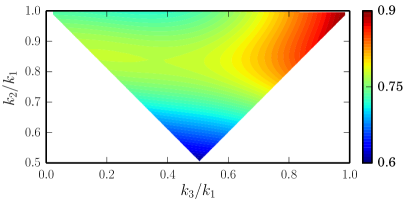
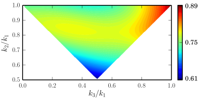
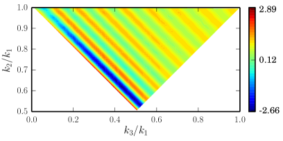
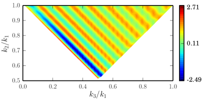
Figure 1: A comparison of the analytical results (on the left) with the numerical results (on the right) for the non-Gaussianity parameter $C_{{}_{\rm NL}}^{\mathcal{R}}({\bm{k}}_{1},{\bm{k}}_{2},{\bm{k}}_{3})$ characterizing the scalar-scalar-tensor three-point function. We have plotted the results for two sets of values of the parameters involved. We have chosen $\mu/M_{{}_{\rm Pl}}=2.512\times 10^{-10}$ in arriving at all these figures. The results in the top row correspond to $b=1.063\times 10^{-2}$ and $f/M_{{}_{\rm Pl}}=7.6346\times 10^{-3}$, which are values that lead to the best fit to the Planck data [57]. The results in the bottom row correspond to $b=5.0\times 10^{-2}$ and $f/M_{{}_{\rm Pl}}=7.6346\times 10^{-4}$. It is clear that the analytical results match the numerical results very well for both these sets of values. In fact, we find that the match is always better than $7\%$ over the range of wavenumbers that we have considered. Note that, as expected, the non-Gaussianity parameter $C_{{}_{\rm NL}}^{\mathcal{R}}({\bm{k}}_{1},{\bm{k}}_{2},{\bm{k}}_{3})$ exhibits more oscillations for smaller values of $f$, as is illustrated by the figures in the bottom row. Also, the strength of these oscillations is more for larger values of $b$.

It is evident from the figure that the analytical results match the numerical ones quite well.

5 The squeezed limit and the consistency relation

In this section, we shall discuss the behavior of the scalar-scalar-tensor three-point function in the so-called squeezed limit. This limit corresponds to the situation where one of the three wavenumbers involved is much smaller than the other two. In such a limit, it is well known that the three-point functions can be written in terms of the two-point functions through a relation known as the consistency condition [14, 75, 76, 77, 78, 79, 80, 81, 82, 85]. This condition primarily arises due to the fact that the amplitude of the long wavelength scalar and tensor modes freeze on supper Hubble scales and hence can be treated as a background as far as the smaller wavelength modes are concerned. In the case of the scalar-scalar-tensor three-point function, when the wavenumber of the tensor mode is considered to be much smaller than the two scalar modes, it is found that the three-point function can be completely expressed in terms of the scalar and tensor power spectra as follows (see, for instance, Refs. [14, 85]):

$$\langle\,{\hat{\mathcal{R}}}_{{\bm{k}}_{1}}(\eta_{\rm e})\,{\hat{\mathcal{R}}}_{{\bm{k}}_{2}}(\eta_{\rm e})\,{\hat{\gamma}}_{m_{3}n_{3}}^{{\bm{k}}_{3}}(\eta_{\rm e})\,\rangle_{k_{3}} = -\,\frac{(2\,\pi)^{5/2}}{4\,k_{1}^{3}\,k_{3}^{3}}\,\left(\frac{n_{{}_{\rm S}}-4}{8}\right)\,{\mathcal{P}}_{{}_{\rm S}}(k_{1})\,{\mathcal{P}}_{{}_{\rm T}}(k_{3})$$ (5.1)

$$\times\,\Pi_{m_{3}n_{3},ij}^{{\bm{k}}_{3}}\,{\hat{n}}_{1i}\,{\hat{n}}_{1j}\,\delta^{3}({\bm{k}}_{1}+{\bm{k}}_{2}),$$

where we have considered ${\bm{k}}_{3}$ to be the squeezed mode. The above condition can essentially be expressed as

$$k^{3}\,k_{3}^{3}\,G_{{\cal R}{\cal R}\gamma}^{m_{3}n_{3}}({\bm{k}},-{\bm{k}},{\bm{k}}_{3}) = -\Pi_{m_{3}n_{3},ij}^{{\bm{k}}_{3}}\,{\hat{n}}_{i}\,{\hat{n}}_{j}\,\frac{(2\,\pi)^{4}}{4}\,\left(\frac{n_{{}_{\rm S}}-4}{8}\right)\,{\mathcal{P}}_{{}_{\rm S}}(k)\,{\mathcal{P}}_{{}_{\rm T}}(k_{3}),$$ (5.2)

with the limit $k_{3}\to 0$ kept in mind. In what follows, using the analytical results we have obtained for the power spectra and the scalar-scalar-tensor cross-correlation, we shall explicitly show that such a consistency relation is indeed satisfied in the axion monodromy model.

Let us now consider the squeezed limit of the three-point function we have arrived at analytically. In the limit ${\bm{k}}_{1}=-{\bm{k}}_{2}={\bm{k}}$ and $k_{3}\rightarrow 0$, at the leading order in $X_{\rm res}$, we find that the three-point function at the order $b$ [i.e.  the sum of the contributions (4.5), (4.7) and (4.10)] reduces to

$$k^{3}\,k_{3}^{3}\,G_{{\cal R}{\cal R}\gamma}^{1(1)}({\bm{k}},-{\bm{k}},{\bm{k}}_{3}) = \Pi_{m_{3}n_{3},ij}^{{\bm{k}}_{3}}\,{\hat{n}}_{i}\,{\hat{n}}_{j}\,\frac{H_{0}^{4}}{8\,i\,M_{{}_{\rm Pl}}^{4}\,\epsilon_{1}^{\ast}}\,\frac{3\,b\,\sqrt{2\,\pi}}{\sqrt{X_{\rm res}}}\,\frac{k}{k_{{}_{{\rm T}1}}}$$ (5.3)

$$\times\,\Biggl{(}{\rm e}^{i\,\phi_{k}/f}\,\left\{\frac{\left[1+\left(k_{{}_{{\rm T}1}}/2\,k\right)\right]^{-i\,X_{\rm res}}}{1+\left(k_{{}_{{\rm T}1}}/2\,k\right)}-1\right\}$$

$$-\,{\rm e}^{-i\,\phi_{k}/f}\,\left\{\frac{\left[1+\left(k_{{}_{{\rm T}1}}/2\,k\right)\right]^{i\,X_{\rm res}}}{1+\left(k_{{}_{{\rm T}1}}/2\,k\right)}-1\right\}\Biggr{)},$$

where, recall that, $k_{{}_{{\rm T}1}}=k_{{}_{\rm T}}-2\,k_{1}$. Hence, in the squeezed limit, $k_{{}_{{\rm T}1}}\rightarrow 0$. Therefore, we can expand the terms $(1+k_{{}_{{\rm T}1}}/2\,k)^{\pm i\,X_{\rm res}}$ in the above equation up to the first order in $k_{{}_{{\rm T}1}}$ to obtain the following expression for the three-point function:

$$k^{3}\,k_{3}^{3}\,G_{{\cal R}{\cal R}\gamma}^{1(1)}({\bm{k}},-{\bm{k}},{\bm{k}}_{3}) = -\Pi_{m_{3}n_{3},ij}^{{\bm{k}}_{3}}\,{\hat{n}}_{i}\,{\hat{n}}_{j}\;\frac{3\,b\,H_{0}^{4}\,\sqrt{2\,\pi}}{8\,M_{{}_{\rm Pl}}^{4}\,\epsilon_{1}^{\ast}}\,X_{\rm res}^{1/2}\,\cos\left(\frac{\phi_{k}}{f}\right).$$ (5.4)

We should mention that, in arriving at this expression, we have ignored a $k$-independent phase.

Let us now turn to the right hand side of the relation (5.2). Up to the linear order in $b$, we can have four combinations of the various terms, given by

$$\left(\frac{n_{{}_{\rm S}}-4}{8}\right)\,{\mathcal{P}}_{{}_{\rm S}}(k)\,{\mathcal{P}}_{{}_{\rm T}}(k_{3}) \simeq \left(\frac{n_{{}_{\rm S}}^{0}-4}{8}\right)\,{\mathcal{P}}_{{}_{\rm S}}^{0}(k)\,{\mathcal{P}}_{{}_{\rm T}}^{0}(k_{3})+\left(\frac{n_{{}_{\rm S}}^{0}-4}{8}\right)\,{\mathcal{P}}_{{}_{\rm S}}^{\rm c}(k)\,{\mathcal{P}}_{{}_{\rm T}}^{0}(k_{3})$$ (5.5)

$$+\,\left(\frac{n_{{}_{\rm S}}^{\rm 0}-4}{8}\right)\,{\mathcal{P}}_{{}_{\rm S}}^{0}(k)\,{\mathcal{P}}_{{}_{\rm T}}^{\rm c}(k_{3})\,+\,\left(\frac{n_{{}_{\rm S}}^{\rm c}}{8}\right)\,{\mathcal{P}}_{{}_{\rm S}}^{0}(k)\,{\mathcal{P}}_{{}_{\rm T}}^{0}(k_{3}),\quad$$

where ${\mathcal{P}}_{{}_{\rm S}}^{0}(k)$ and ${\mathcal{P}}_{{}_{\rm T}}^{0}(k)$ and $n_{{}_{\rm S}}^{0}$ are the scalar and the tensor power spectra and the scalar spectral index, respectively, which arise in the absence of the oscillations in the axion monodromy model. Note that ${\mathcal{P}}_{{}_{\rm T}}^{\rm c}(k)$ involves terms of order $d_{k}$ and, as we have discussed before, these terms are of lower order when compared to the other terms involving $c_{k}$. Hence, for consistency, we can ignore the contribution due to ${\mathcal{P}}_{{}_{\rm T}}^{\rm c}(k)$ in the above equation. Therefore, we finally obtain that

$$\left(\frac{n_{{}_{\rm S}}-4}{8}\right)\,{\mathcal{P}}_{{}_{\rm S}}(k)\,{\mathcal{P}}_{{}_{\rm T}}(k_{3}) \simeq \left(\frac{n_{{}_{\rm S}}^{0}-4}{8}\right)\,{\mathcal{P}}_{{}_{\rm S}}^{0}(k)\,{\mathcal{P}}_{{}_{\rm T}}^{0}(k_{3})+\left(\frac{n_{{}_{\rm S}}^{0}-4}{8}\right)\,{\mathcal{P}}_{{}_{\rm S}}^{\rm c}(k)\,{\mathcal{P}}_{{}_{\rm T}}^{0}(k_{3})$$ (5.6)

$$+\,\left(\frac{n_{{}_{\rm S}}^{\rm c}}{8}\right)\,{\mathcal{P}}_{{}_{\rm S}}^{0}(k)\,{\mathcal{P}}_{{}_{\rm T}}^{0}(k_{3}).$$

The first term in the above expression is the slow roll term for which the consistency relation involving the $b=0$ contribution to the scalar-scalar-tensor cross correlation, viz.  $G_{{\cal R}{\cal R}\gamma}^{1(0)}({\bm{k}}_{1},{\bm{k}}_{2},{\bm{k}}_{3})$, can be verified easily [70, 85]. On evaluating the remaining two terms, we find that the one involving $n_{{}_{\rm S}}^{\rm c}$ is of leading order, as the other term is suppressed relative to this by a factor of $X_{\rm res}$. Hence, at the leading order in $b$, we can replace $\left[\left(n_{{}_{\rm S}}-4\right)/8\right]\,{\mathcal{P}}_{{}_{\rm S}}(k)\,{\mathcal{P}}_{{}_{\rm T}}(k_{3})$ by $\left(n_{{}_{\rm S}}^{\rm c}/8\right)\,{\mathcal{P}}_{{}_{\rm S}}^{0}(k)\,{\mathcal{P}}_{{}_{\rm T}}^{0}(k_{3})$ in Eq. (5.2). Upon making this replacement, the consistency relation at the linear order in $b$ can be written as

$$k^{3}\,k_{3}^{3}\,G_{{\mathcal{R}}{\mathcal{R}}\gamma}^{1(1)}({\bm{k}},-{\bm{k}},{\bm{k}}_{3})=-\Pi^{{\bm{k}}_{3}}_{m_{3}n_{3},ij}\,{\hat{n}}_{1i}\,{\hat{n}}_{1j}\,\frac{(2\,\pi)^{4}}{4}\,\left(\frac{n_{{}_{\rm S}}^{\rm c}}{8}\right)\,{\mathcal{P}}_{{}_{\rm S}}^{0}\,{\mathcal{P}}_{{}_{\rm T}}^{0}.$$ (5.7)

Now, on substituting the expression for $n_{{}_{\rm S}}^{c}$ [cf. Eqs. (2.37)] and the slow roll amplitudes for the scalar and tensor power spectra [cf. Eqs. (2.35) and (2.51)] in the above expression, we find that the resultant expression is the same as that obtained in Eq. (5.4), up to a $k$-independent phase. This implies that the consistency relation is valid in the axion monodromy model even in the presence of persistent oscillations in the two as well as the three-point functions [85].

6 Discussion

The axion monodromy model is described by a linear potential with small periodic modulations. The modulations in the potential lead to oscillations in the slow roll parameters. These oscillations associated with the background resonate with the oscillations of the scalar and tensor perturbations at sub-Hubble scales for suitable values of the parameters of the model. This resonance leads to persistent oscillations in the two and three-point functions. The scalar and tensor power spectra as well as the scalar bi-spectrum have been analytically evaluated earlier in the axion monodromy model under certain approximations.

In terms of their hierarchy, after the scalar bi-spectrum, the scalar-scalar-tensor cross-correlation proves to be the most important of the three-point functions. In this work, we have analytically calculated the scalar-scalar-tensor three-point function in the axion monodromy model in the same approximation under which the scalar and tensor power spectra and the scalar bi-spectrum had been evaluated earlier. We find that the analytical results we have obtained match the corresponding numerical results very well for a range of the parameters involved. Subsequently, using the analytical results, we have also been able to explicitly verify the consistency relation governing the three-point function.

The template that we have obtained here can be used to compare the inflationary models with the CMB data at the level of three-point functions involving the tensor perturbations (in this context, see the recent work, Ref. [89]). Clearly, it will be interesting to extend our analysis to the scalar-tensor-tensor three-point function as well as the tensor bi-spectrum. We find that the tensor bi-spectrum can be easily evaluated using the methods adopted here. However, comparison with the corresponding numerical results suggest that these methods do not prove to be adequate to evaluate the scalar-tensor-tensor three-point function to the same level of accuracy. Also, for instance, the consistency relation for the three-point function also does not seem to hold under these approximations. These approximations need to be extended in order to evaluate the scalar-tensor-tensor cross-correlation analytically to a good level of accuracy. We are currently investigating this issue.

References

- [1] M. J. Mortonson, H. V. Peiris, and R. Easther, Bayesian Analysis of Inflation: Parameter Estimation for Single Field Models, Phys. Rev. D83 (2011) 043505, [arXiv:1007.4205].
- [2] R. Easther and H. V. Peiris, Bayesian Analysis of Inflation II: Model Selection and Constraints on Reheating, Phys. Rev. D85 (2012) 103533, [arXiv:1112.0326].
- [3] J. Norena, C. Wagner, L. Verde, H. V. Peiris, and R. Easther, Bayesian Analysis of Inflation III: Slow Roll Reconstruction Using Model Selection, Phys. Rev. D86 (2012) 023505, [arXiv:1202.0304].
- [4] J. Martin, C. Ringeval, and R. Trotta, Hunting Down the Best Model of Inflation with Bayesian Evidence, Phys. Rev. D83 (2011) 063524, [arXiv:1009.4157].
- [5] J. Martin, C. Ringeval, and V. Vennin, Encyclopædia Inflationaris, Phys.Dark Univ. 5-6 (2014) 75–235, [arXiv:1303.3787].
- [6] J. Martin, C. Ringeval, R. Trotta, and V. Vennin, The Best Inflationary Models After Planck, JCAP 1403 (2014) 039, [arXiv:1312.3529].
- [7] J. Martin, C. Ringeval, R. Trotta, and V. Vennin, Compatibility of Planck and BICEP2 in the Light of Inflation, Phys. Rev. D90 (2014), no. 6 063501, [arXiv:1405.7272].
- [8] J. Martin, C. Ringeval, and V. Vennin, How Well Can Future CMB Missions Constrain Cosmic Inflation?, JCAP 1410 (2014), no. 10 038, [arXiv:1407.4034].
- [9] Planck Collaboration, P. A. R. Ade et al., Planck 2015 results. XX. Constraints on inflation, arXiv:1502.02114.
- [10] A. Gangui, F. Lucchin, S. Matarrese, and S. Mollerach, The Three point correlation function of the cosmic microwave background in inflationary models, Astrophys. J. 430 (1994) 447–457, [astro-ph/9312033].
- [11] A. Gangui, NonGaussian effects in the cosmic microwave background from inflation, Phys. Rev. D50 (1994) 3684–3691, [astro-ph/9406014].
- [12] A. Gangui and J. Martin, Cosmic microwave background bispectrum and slow roll inflation, Mon. Not. Roy. Astron. Soc. 313 (2000) 323, [astro-ph/9908009].
- [13] L.-M. Wang and M. Kamionkowski, The Cosmic microwave background bispectrum and inflation, Phys. Rev. D61 (2000) 063504, [astro-ph/9907431].
- [14] J. M. Maldacena, Non-Gaussian features of primordial fluctuations in single field inflationary models, JHEP 05 (2003) 013, [astro-ph/0210603].
- [15] D. Seery and J. E. Lidsey, Primordial non-Gaussianities in single field inflation, JCAP 0506 (2005) 003, [astro-ph/0503692].
- [16] X. Chen, Running non-Gaussianities in DBI inflation, Phys. Rev. D72 (2005) 123518, [astro-ph/0507053].
- [17] X. Chen, M.-x. Huang, S. Kachru, and G. Shiu, Observational signatures and non-Gaussianities of general single field inflation, JCAP 0701 (2007) 002, [hep-th/0605045].
- [18] D. Langlois, S. Renaux-Petel, D. A. Steer, and T. Tanaka, Primordial fluctuations and non-Gaussianities in multi-field DBI inflation, Phys. Rev. Lett. 101 (2008) 061301, [arXiv:0804.3139].
- [19] D. Langlois, S. Renaux-Petel, D. A. Steer, and T. Tanaka, Primordial perturbations and non-Gaussianities in DBI and general multi-field inflation, Phys. Rev. D78 (2008) 063523, [arXiv:0806.0336].
- [20] X. Chen, Primordial Non-Gaussianities from Inflation Models, Adv. Astron. 2010 (2010) 638979, [arXiv:1002.1416].
- [21] Y. Wang, Inflation, Cosmic Perturbations and Non-Gaussianities, Commun.Theor.Phys. 62 (2014) 109–166, [arXiv:1303.1523].
- [22] J. Martin, The Observational Status of Cosmic Inflation after Planck, 2015. arXiv:1502.05733.
- [23] E. Komatsu and D. N. Spergel, Acoustic signatures in the primary microwave background bispectrum, Phys. Rev. D63 (2001) 063002, [astro-ph/0005036].
- [24] E. Komatsu, D. N. Spergel, and B. D. Wandelt, Measuring primordial non-Gaussianity in the cosmic microwave background, Astrophys. J. 634 (2005) 14–19, [astro-ph/0305189].
- [25] D. Babich and M. Zaldarriaga, Primordial bispectrum information from CMB polarization, Phys. Rev. D70 (2004) 083005, [astro-ph/0408455].
- [26] M. Liguori, F. K. Hansen, E. Komatsu, S. Matarrese, and A. Riotto, Testing primordial non-gaussianity in cmb anisotropies, Phys. Rev. D73 (2006) 043505, [astro-ph/0509098].
- [27] C. Hikage, E. Komatsu, and T. Matsubara, Primordial Non-Gaussianity and Analytical Formula for Minkowski Functionals of the Cosmic Microwave Background and Large-scale Structure, Astrophys. J. 653 (2006) 11–26, [astro-ph/0607284].
- [28] J. R. Fergusson and E. P. S. Shellard, Primordial non-Gaussianity and the CMB bispectrum, Phys. Rev. D76 (2007) 083523, [astro-ph/0612713].
- [29] A. P. S. Yadav, E. Komatsu, and B. D. Wandelt, Fast Estimator of Primordial Non-Gaussianity from Temperature and Polarization Anisotropies in the Cosmic Microwave Background, Astrophys. J. 664 (2007) 680–686, [astro-ph/0701921].
- [30] P. Creminelli, L. Senatore, and M. Zaldarriaga, Estimators for local non-Gaussianities, JCAP 0703 (2007) 019, [astro-ph/0606001].
- [31] A. P. S. Yadav and B. D. Wandelt, Evidence of Primordial Non-Gaussianity (f(NL)) in the Wilkinson Microwave Anisotropy Probe 3-Year Data at 2.8sigma, Phys. Rev. Lett. 100 (2008) 181301, [arXiv:0712.1148].
- [32] C. Hikage, T. Matsubara, P. Coles, M. Liguori, F. K. Hansen, and S. Matarrese, Limits on Primordial Non-Gaussianity from Minkowski Functionals of the WMAP Temperature Anisotropies, Mon. Not. Roy. Astron. Soc. 389 (2008) 1439–1446, [arXiv:0802.3677].
- [33] O. Rudjord, F. K. Hansen, X. Lan, M. Liguori, D. Marinucci, and S. Matarrese, An Estimate of the Primordial Non-Gaussianity Parameter f_NL Using the Needlet Bispectrum from WMAP, Astrophys. J. 701 (2009) 369–376, [arXiv:0901.3154].
- [34] K. M. Smith, L. Senatore, and M. Zaldarriaga, Optimal limits on fNLlocal from WMAP 5-year data, JCAP 0909 (2009) 006, [arXiv:0901.2572].
- [35] J. Smidt, A. Amblard, C. T. Byrnes, A. Cooray, A. Heavens, and D. Munshi, CMB Constraints on Primordial non-Gaussianity from the Bispectrum (fNL) and Trispectrum (gNL and ) and a New Consistency Test of Single-Field Inflation, Phys. Rev. D81 (2010) 123007, [arXiv:1004.1409].
- [36] J. R. Fergusson, M. Liguori, and E. P. S. Shellard, The CMB Bispectrum, JCAP 1212 (2012) 032, [arXiv:1006.1642].
- [37] M. Liguori, E. Sefusatti, J. R. Fergusson, and E. P. S. Shellard, Primordial non-Gaussianity and Bispectrum Measurements in the Cosmic Microwave Background and Large-Scale Structure, Adv. Astron. 2010 (2010) 980523, [arXiv:1001.4707].
- [38] A. P. S. Yadav and B. D. Wandelt, Primordial Non-Gaussianity in the Cosmic Microwave Background, Adv. Astron. 2010 (2010) 565248, [arXiv:1006.0275].
- [39] E. Komatsu, Hunting for Primordial Non-Gaussianity in the Cosmic Microwave Background, Class. Quant. Grav. 27 (2010) 124010, [arXiv:1003.6097].
- [40] Planck Collaboration, P. A. R. Ade et al., Planck 2015 results. XVII. Constraints on primordial non-Gaussianity, arXiv:1502.01592.
- [41] R. K. Jain, P. Chingangbam, J.-O. Gong, L. Sriramkumar, and T. Souradeep, Punctuated inflation and the low CMB multipoles, JCAP 0901 (2009) 009, [arXiv:0809.3915].
- [42] R. K. Jain, P. Chingangbam, L. Sriramkumar, and T. Souradeep, The tensor-to-scalar ratio in punctuated inflation, Phys. Rev. D82 (2010) 023509, [arXiv:0904.2518].
- [43] D. K. Hazra, M. Aich, R. K. Jain, L. Sriramkumar, and T. Souradeep, Primordial features due to a step in the inflaton potential, JCAP 1010 (2010) 008, [arXiv:1005.2175].
- [44] D. K. Hazra, A. Shafieloo, and T. Souradeep, Primordial power spectrum: a complete analysis with the WMAP nine-year data, JCAP 1307 (2013) 031, [arXiv:1303.4143].
- [45] D. K. Hazra, A. Shafieloo, and T. Souradeep, Primordial power spectrum from Planck, JCAP 1411 (2014), no. 11 011, [arXiv:1406.4827].
- [46] P. Hunt and S. Sarkar, Reconstruction of the primordial power spectrum of curvature perturbations using multiple data sets, JCAP 1401 (2014), no. 01 025, [arXiv:1308.2317].
- [47] P. Hunt and S. Sarkar, Search for features in the spectrum of primordial perturbations using Planck and other datasets, arXiv:1510.03338.
- [48] D. K. Hazra, A. Shafieloo, G. F. Smoot, and A. A. Starobinsky, Inflation with Whip-Shaped Suppressed Scalar Power Spectra, Phys. Rev. Lett. 113 (2014), no. 7 071301, [arXiv:1404.0360].
- [49] D. K. Hazra, A. Shafieloo, G. F. Smoot, and A. A. Starobinsky, Wiggly Whipped Inflation, JCAP 1408 (2014) 048, [arXiv:1405.2012].
- [50] J. Martin and C. Ringeval, Superimposed oscillations in the WMAP data?, Phys. Rev. D69 (2004) 083515, [astro-ph/0310382].
- [51] J. Martin and C. Ringeval, Addendum to ‘Superimposed oscillations in the WMAP data?’, Phys. Rev. D69 (2004) 127303, [astro-ph/0402609].
- [52] J. Martin and C. Ringeval, Exploring the superimposed oscillations parameter space, JCAP 0501 (2005) 007, [hep-ph/0405249].
- [53] M. Zarei, Short Distance Physics and Initial State Effects on the CMB Power Spectrum and Cosmological Constant, Phys. Rev. D78 (2008) 123502, [arXiv:0809.4312].
- [54] C. Pahud, M. Kamionkowski, and A. R. Liddle, Oscillations in the inflaton potential?, Phys. Rev. D79 (2009) 083503, [arXiv:0807.0322].
- [55] T. Kobayashi and F. Takahashi, Running Spectral Index from Inflation with Modulations, JCAP 1101 (2011) 026, [arXiv:1011.3988].
- [56] P. D. Meerburg, D. N. Spergel, and B. D. Wandelt, Searching for oscillations in the primordial power spectrum. I. Perturbative approach, Phys.Rev. D89 (2014), no. 6 063536, [arXiv:1308.3704].
- [57] P. D. Meerburg and D. N. Spergel, Searching for oscillations in the primordial power spectrum. II. Constraints from Planck data, Phys.Rev. D89 (2014), no. 6 063537, [arXiv:1308.3705].
- [58] R. Flauger, L. McAllister, E. Pajer, A. Westphal, and G. Xu, Oscillations in the CMB from Axion Monodromy Inflation, JCAP 1006 (2010) 009, [arXiv:0907.2916].
- [59] M. Aich, D. K. Hazra, L. Sriramkumar, and T. Souradeep, Oscillations in the inflaton potential: Complete numerical treatment and comparison with the recent and forthcoming CMB datasets, Phys. Rev. D87 (2013) 083526, [arXiv:1106.2798].
- [60] H. Peiris, R. Easther, and R. Flauger, Constraining Monodromy Inflation, JCAP 1309 (2013) 018, [arXiv:1303.2616].
- [61] R. Easther and R. Flauger, Planck Constraints on Monodromy Inflation, JCAP 1402 (2014) 037, [arXiv:1308.3736].
- [62] P. D. Meerburg, Alleviating the tension at low through axion monodromy, Phys. Rev. D90 (2014), no. 6 063529, [arXiv:1406.3243].
- [63] D. K. Hazra, L. Sriramkumar, and J. Martin, BINGO: A code for the efficient computation of the scalar bi-spectrum, JCAP 1305 (2013) 026, [arXiv:1201.0926].
- [64] R. Flauger and E. Pajer, Resonant Non-Gaussianity, JCAP 1101 (2011) 017, [arXiv:1002.0833].
- [65] J. R. Fergusson, H. F. Gruetjen, E. P. S. Shellard, and M. Liguori, Combining power spectrum and bispectrum measurements to detect oscillatory features, Phys. Rev. D91 (2015), no. 2 023502, [arXiv:1410.5114].
- [66] J. R. Fergusson, H. F. Gruetjen, E. P. S. Shellard, and B. Wallisch, Polyspectra searches for sharp oscillatory features in cosmic microwave sky data, Phys. Rev. D91 (2015), no. 12 123506, [arXiv:1412.6152].
- [67] X. Gao, T. Kobayashi, M. Shiraishi, M. Yamaguchi, J. Yokoyama, and S. Yokoyama, Full bispectra from primordial scalar and tensor perturbations in the most general single-field inflation model, PTEP 2013 (2013) 053E03, [arXiv:1207.0588].
- [68] L. Dai, D. Jeong, and M. Kamionkowski, Seeking Inflation Fossils in the Cosmic Microwave Background, Phys. Rev. D87 (2013), no. 10 103006, [arXiv:1302.1868].
- [69] V. Sreenath, R. Tibrewala, and L. Sriramkumar, Numerical evaluation of the three-point scalar-tensor cross-correlations and the tensor bi-spectrum, JCAP 1312 (2013) 037, [arXiv:1309.7169].
- [70] S. Kundu, Non-Gaussianity Consistency Relations, Initial States and Back-reaction, JCAP 1404 (2014) 016, [arXiv:1311.1575].
- [71] E. Dimastrogiovanni, M. Fasiello, D. Jeong, and M. Kamionkowski, Inflationary tensor fossils in large-scale structure, JCAP 1412 (2014) 050, [arXiv:1407.8204].
- [72] E. Dimastrogiovanni, M. Fasiello, and M. Kamionkowski, Imprints of Massive Primordial Fields on Large-Scale Structure, arXiv:1504.05993.
- [73] J. M. Maldacena and G. L. Pimentel, On graviton non-Gaussianities during inflation, JHEP 09 (2011) 045, [arXiv:1104.2846].
- [74] X. Gao, T. Kobayashi, M. Yamaguchi, and J. Yokoyama, Primordial non-Gaussianities of gravitational waves in the most general single-field inflation model, Phys. Rev. Lett. 107 (2011) 211301, [arXiv:1108.3513].
- [75] P. Creminelli and M. Zaldarriaga, Single field consistency relation for the 3-point function, JCAP 0410 (2004) 006, [astro-ph/0407059].
- [76] C. Cheung, A. L. Fitzpatrick, J. Kaplan, and L. Senatore, On the consistency relation of the 3-point function in single field inflation, JCAP 0802 (2008) 021, [arXiv:0709.0295].
- [77] S. Renaux-Petel, On the squeezed limit of the bispectrum in general single field inflation, JCAP 1010 (2010) 020, [arXiv:1008.0260].
- [78] J. Ganc and E. Komatsu, A new method for calculating the primordial bispectrum in the squeezed limit, JCAP 1012 (2010) 009, [arXiv:1006.5457].
- [79] P. Creminelli, G. D’Amico, M. Musso, and J. Norena, The (not so) squeezed limit of the primordial 3-point function, JCAP 1111 (2011) 038, [arXiv:1106.1462].
- [80] D. Chialva, Enhanced CMBR non-Gaussianities from Lorentz violation, JCAP 1201 (2012) 037, [arXiv:1106.0040].
- [81] K. Schalm, G. Shiu, and T. van der Aalst, Consistency condition for inflation from (broken) conformal symmetry, JCAP 1303 (2013) 005, [arXiv:1211.2157].
- [82] E. Pajer, F. Schmidt, and M. Zaldarriaga, The Observed Squeezed Limit of Cosmological Three-Point Functions, Phys.Rev. D88 (2013), no. 8 083502, [arXiv:1305.0824].
- [83] Z. Kenton and D. J. Mulryne, The squeezed limit of the bispectrum in multi-field inflation, JCAP 1510 (2015), no. 10 018, [arXiv:1507.08629].
- [84] Z. Kenton and D. J. Mulryne, The Separate Universe Approach to Soft Limits, arXiv:1605.03435.
- [85] V. Sreenath and L. Sriramkumar, Examining the consistency relations describing the three-point functions involving tensors, JCAP 1410 (2014), no. 10 021, [arXiv:1406.1609].
- [86] N. Kundu, A. Shukla, and S. P. Trivedi, Constraints from Conformal Symmetry on the Three Point Scalar Correlator in Inflation, JHEP 04 (2015) 061, [arXiv:1410.2606].
- [87] N. Kundu, A. Shukla, and S. P. Trivedi, Ward Identities for Scale and Special Conformal Transformations in Inflation, JHEP 01 (2016) 046, [arXiv:1507.06017].
- [88] I. S. Gradshteyn and I. M. Ryzhik, Table of Integrals, Series, and Products. Academic Press, New York, 7th ed., 2007.
- [89] P. D. Meerburg, J. Meyers, A. van Engelen, and Y. Ali-Haïmoud, On CMB B-Mode Non-Gaussianity, arXiv:1603.02243.