New Complexiton Solutions of the KdV and Coupled KdV Equations

Abstract

A new approach to double-sub equation method is introduced to construct novel solutions for the nonlinear partial differential equations. It is applied to the Korteweg-de Vries (KdV) equation and yields new complexiton solutions of both the KdV and coupled KdV equations. The graphs of the solutions are also illustrated.

Keywords: Complexiton solution, KdV equation, Coupled KdV equation, Double-sub equation method

PACS 02.30.Ik, 02.30.Jr, 05.45.Yv

1 Introduction

The Korteweg de Vries (KdV) equation

$$u_{t}+\zeta uu_{x}+\rho u_{xxx}=0,\quad\quad\zeta,\rho\,\mathrm{arbitrary}\,\mathrm{constants}.$$ (1.1)

is a famous $(1+1)$-dimensional integrable nonlinear partial differential equation which models waves on shallow water surfaces, ion acoustic waves in plasma, acoustic waves on a crystal lattice etc. It is introduced by Boussinesq [1] and rediscovered by Korteweg and de-Vries [2]. Since then there has been a huge interest on analysis of its rich structure- Lax pairs [3], symmetries [4], Bäcklund transformations [5], and so on, and finding its solutions. Researches on exploring the solutions inspired important methods like inverse scattering method [6]-[8], Hirota direct method [9]-[12], and Painlevé expansion [13]-[15].

The KdV equation has various type of solutions like soliton [9], and negaton, positon [16], and complexiton solutions [17]-[19]. There is a great interest to obtain new type of solutions hence several solution methods whose efficiency should also be discussed are constructed. One of them is the sub-ordinary differential equation method [20]-[22]. It was improved and had a new name ’double-sub equation method’ in [23]. The authors of [23] claimed that by using this method one can get complexiton solutions combining Jacobi elliptic functions and elementary functions. They applied this method to the KdV and mKdV equations. In [24], it was shown that the solutions found in [23] are just constant solutions. But the method can still be used to find solutions of nonlinear partial differential equations.

In this paper, to get a wider class of solutions including complexiton solutions depending on two independent variables we use an ansatz different than the one in [23] for the form of the solution. In fact, we really obtain new complexiton solutions of the KdV equation.

Another set of the solutions yielded in this paper is for the coupled KdV equation. One type of the coupled KdV equations

$$U_{t}+\zeta UU_{x}-\zeta VV_{x}+\rho U_{xxx} =0$$ (1.2)

$$V_{t}+\zeta UV_{x}+\zeta VU_{x}+\rho V_{xxx} =0$$

can be obtained from the KdV equation by simply using the transformation $u(x,t)=U(x,t)+\.{i}V(x,t)$ and separating the real and imaginary parts. There are many coupled KdV systems like the Hirota and Satsuma system [25], the Drinfeld and Sokolov model [26], the Fuchssteiner equation [27], the Nutku-Og̃uz model [28], the degenerate coupled KdV systems [29], [30], and so on. The coupled KdV system (1.2) used in this paper was derived as a special case of the general coupled KdV systems obtained from the two layer model of the atmospheric dynamical systems [31] and two-component Bose-Einstein condensates [32]. Even the complexiton solutions have been studied for several years, in our knowledge, there was no non-singular complexiton solution until the work of Hu et al. [33]. They discovered non-singular complexiton solutions of (1.2) by using the iterative Darboux transformations. Afterwards, Yang and Mao in [34] obtained non-singular complexiton solutions of (1.2) different from the solutions in [33] by applying Hirota’s direct method and conjugate number form of exponential functions. In this paper, investigating solutions of the KdV equation by the new approach reveals novel non-singular complexiton solutions of the coupled KdV equation different than the other solutions obtained before [33], [34].

This paper is organized as follows. In Section II, we introduce the new approach to double-sub equation method and apply it to the KdV equation. Solutions depending on one and two independent variables are given. The latter case is analyzed in detail. The complexiton solutions of the coupled KdV equation obtained during the application of the new approach to the KdV equation are also given. Graphs of the solutions are illustrated. In Section III, asymptotic behaviors of the solutions are discussed.

2 A New Approach

In [23] the authors presented a method called double-sub equation method, which we will call it as Ma’s approach. They assume the form of the solution as

$$u(x,t)=a_{0}+\frac{a_{1}F(\xi)+a_{2}G(\eta)}{\mu_{0}+\mu_{1}F(\xi)+\mu_{2}G(\eta)}+\frac{a_{3}F(\xi)^{2}+a_{4}F(\xi)G(\eta)+a_{5}G(\eta)^{2}}{(\mu_{0}+\mu_{1}F(\xi)+\mu_{2}G(\eta))^{2}},$$ (2.1)

where the functions $F(\xi)$ and $G(\eta)$ satisfies first order ODEs

$$(F^{\prime})^{2}(\xi)=\alpha_{1}+\beta_{1}F^{2}(\xi)+\gamma_{1}F^{4}(\xi),\quad(G^{\prime})^{2}(\eta)=\alpha_{2}+\beta_{2}G^{2}(\eta)$$ (2.2)

where $\xi=k_{1}(x-c_{1}t)$ and $\eta=k_{2}(x-c_{2}t)$ with unknown constants $a_{i}$, $i=0,1,\ldots,5$; $\mu_{j}$, $j=0,1,2$; $k_{m}$, $c_{m}$, $m=1,2$ that will be determined. As noted before, the solutions in [23] are constants but indeed, this approach gives non-constant but not original solutions. Some of the non-constant solutions of the KdV equation which can be obtained by Ma’s approach are the followings.

If $\displaystyle a_{1}=a_{2}=a_{4}=a_{5}=\mu_{1}=\mu_{2}=0,a_{3}=-12\rho k_{1}^{2}\mu_{0}^{2}\gamma_{1}/\zeta$, and $c_{1}=4\rho k_{1}^{2}\beta_{1}+a_{0}\zeta$, we obtain the solution

$$u(x,t)=a_{0}-\frac{24\rho\alpha_{1}\gamma_{1}k_{1}^{2}}{\zeta\omega}\mathrm{sn}^{2}\Big{(}\frac{\sqrt{2\omega}}{2}\xi+\theta_{1},k\Big{)},$$ (2.3)

where $\xi=k_{1}(x-c_{1}t)$, $k=\sqrt{-2\gamma_{1}\alpha_{1}}/\sqrt{2\gamma_{1}\alpha_{1}+\beta_{1}\omega}$ with $\omega=-\beta_{1}+\sqrt{\beta_{1}^{2}-4\gamma_{1}\alpha_{1}}$, $c_{1}=4\rho k_{1}^{2}\beta_{1}+a_{0}\zeta$, and $\theta_{1}$ is any constant. This solution can easily be obtained by using symmetry reduction.

Another solution occurs when $\displaystyle a_{1}=a_{3}=a_{4}=\mu_{1}=\alpha_{2}=0,a_{0}=(12c_{2}\mu_{2}-\zeta a_{2})/12\zeta\mu_{2},a_{5}=-a_{2}\mu_{2}$, and $\displaystyle\beta_{2}=\zeta a_{2}/12\rho k_{2}^{2}\mu_{2}$. We get

$$u(x,t)=\frac{12c_{2}\mu_{2}-\zeta a_{2}}{12\zeta\mu_{2}}+\frac{a_{2}e^{\pm\frac{\sqrt{\zeta a_{2}}}{2k_{2}\sqrt{3\rho\mu_{2}}}(\eta+\theta_{1})}}{\mu_{0}+\mu_{2}e^{\pm\frac{\sqrt{\zeta a_{2}}}{2k_{2}\sqrt{3\rho\mu_{2}}}(\eta+\theta_{1})}}-\frac{a_{2}\mu_{2}e^{\pm\frac{\sqrt{\zeta a_{2}}}{k_{2}\sqrt{3\rho\mu_{2}}}(\eta+\theta_{1})}}{\Big{(}\mu_{0}+\mu_{2}e^{\pm\frac{\sqrt{\zeta a_{2}}}{2k_{2}\sqrt{3\rho\mu_{2}}}(\eta+\theta_{1})}\Big{)}^{2}},$$

where $\eta=k_{2}(x-c_{2}t)$ and $\theta_{1}$ is any constant.

Now we explain our approach to double-sub equation method which produces novel complexiton solutions depending on two independent variables and also periodic and solitary wave solutions. Let

$$\Lambda(u,u_{x},u_{t},u_{xx},...)=0$$ (2.4)

be a partial differential equation in two independent variables. Assume the following ansatz for the solutions of (2.4)

$$u(x,t)=a_{0}+\frac{\kappa_{1}+a_{1}F(\xi)+a_{2}G(\eta)}{\mu_{0}+\mu_{1}F^{\prime}(\xi)+\mu_{2}G^{\prime}(\eta)}+\frac{\kappa_{2}+a_{3}F(\xi)^{2}+a_{4}F(\xi)G(\eta)+a_{5}G(\eta)^{2}}{(\mu_{0}+\mu_{1}F^{\prime}(\xi)+\mu_{2}G^{\prime}(\eta))^{2}},$$ (2.5)

where $\mu_{i}$, $i=0,1,2$; $a_{j}$, $j=0,\ldots,5$, $\kappa_{m}$, $m=1,2$ are unknown constants. Here the functions $F(\xi)$ and $G(\eta)$ satisfy the following ODEs,

$$(F^{\prime})^{2}(\xi)=\alpha_{1}+\beta_{1}F^{2}(\xi)+\gamma_{1}F^{4}(\xi),\quad(G^{\prime})^{2}(\eta)=\alpha_{2}+\beta_{2}G^{2}(\eta)+\gamma_{2}G^{4}(\eta)$$ (2.6)

with $\xi=k_{1}(x-c_{1}t)$ and $\eta=k_{2}(x-c_{2}t)$, and $\alpha_{i}$, $\beta_{i}$, $\gamma_{i}$, $k_{i}$, $c_{i}$, $i=1,2$ are unknown constants to be determined. The ansatz for the form of the solution used here is different than (2.1) so that it gives wider class of solutions including the solutions depending on two independent variables $\xi$ and $\eta$. Substituting (2.5) into (1.1) and using the constraints (2.6) give a system of equations with respect to $F^{i}G^{j}F^{\prime r}G^{\prime p}$, $0\leq i,j\leq 10$; $r,p=0,1$. We set the coefficients of $F^{i}G^{j}F^{\prime r}G^{\prime p}$, $0\leq i,j\leq 10$; $r,p=0,1$ to vanish. This yields a set of equations in terms of the unknowns, $a_{i}$, $i=0,1,\ldots,5$; $\mu_{j}$, $j=0,1,2$; $\kappa_{l}$, $c_{l}$, $k_{l}$, $\alpha_{l}$, $\beta_{l}$, and $\gamma_{l}$, $l=1,2$. By the help of MAPLE, we solve these equations and obtain solutions depending on one independent variable and two independent variables. Indeed, the latter case is more interesting and there are not so many such kind of solutions. Therefore in the next section we will just present two examples related to the first case then focus on the solutions having two independent variables.

2.1 Solutions depending on one independent variable

Some solutions of the KdV equation depending on one independent variable obtained by the new approach are the followings.

Let $a_{1}=a_{2}=a_{4}=a_{5}=\kappa_{1}=\kappa_{2}=\mu_{0}=\mu_{2}=0$, $\displaystyle a_{3}=(48\rho\alpha_{1}\gamma_{1}\mu_{1}^{2}k_{1}^{2}-12\rho\beta_{1}^{2}\mu_{1}^{2}k_{1}^{2})/\zeta$, and $c_{1}=-8\rho\beta_{1}k_{1}^{2}+a_{0}\zeta$. Then the solution is

$$u(x,t)=a_{0}+\frac{48\rho\mu_{1}^{2}k_{1}^{2}(4\gamma_{1}\alpha_{1}-\beta_{1}^{2})\mathrm{sn}^{2}(\delta\xi+A_{1},k)}{\mu_{1}^{2}(-2\beta_{1}+2\sqrt{\beta_{1}^{2}-4\gamma_{1}\alpha_{1}})\mathrm{cn}^{2}(\delta\xi+A_{1},k)\mathrm{dn}^{2}(\delta\xi+A_{1},k)},$$

where

$$\delta=\frac{1}{2}\sqrt{-2\beta_{1}+2\sqrt{\beta_{1}^{2}-4\gamma_{1}\alpha_{1}}},\quad\displaystyle k=\frac{\sqrt{-2(2\gamma_{1}\alpha_{1}-\beta_{1}^{2}+\beta_{1}\sqrt{\beta_{1}^{2}-4\gamma_{1}\alpha_{1}})\gamma_{1}\alpha_{1}}}{2\gamma_{1}\alpha_{1}-\beta_{1}^{2}+\beta_{1}\sqrt{\beta_{1}^{2}-4\gamma_{1}\alpha_{1}}},$$

and $A_{1}$ is an arbitrary constant. This solution is a periodic solution.

Now let us take the parameters as $a_{1}=a_{2}=\kappa_{1}=\kappa_{2}=\mu_{0}=\gamma_{1}=\gamma_{2}=0$,

$$a_{3}=-\frac{4\rho\mu_{1}^{2}\beta_{1}^{2}k_{1}^{2}}{3\zeta},\quad a_{4}=\frac{8\rho\mu_{1}\beta_{1}^{2}k_{1}^{3}\mu_{2}}{9k_{2}\zeta},\quad a_{5}=-\frac{4\rho\mu_{2}^{2}\beta_{1}^{2}k_{1}^{4}}{27\zeta k_{2}^{2}}$$

$$\alpha_{2}=\frac{\alpha_{1}\mu_{1}^{2}}{\mu_{2}^{2}},\quad\beta_{2}=\frac{\beta_{1}k_{1}^{2}}{9k_{2}^{2}},\quad c_{2}=3c_{1}+\frac{16}{9}\rho\beta_{1}k_{1}^{2}-2\zeta a_{0}.$$ (2.7)

Choosing $\alpha_{1}>0$ and $\beta_{1}>0$, we obtain the following non-constant functions $F$ and $G$ from (2.6),

$$F(\xi)=\pm\sqrt{\frac{\alpha_{1}}{\beta_{1}}}\sinh(\sqrt{\beta_{1}}(\xi+A_{1})),\quad G(\eta)=\pm\sqrt{\frac{\alpha_{2}}{\beta_{2}}}\sinh(\sqrt{\beta_{2}}(\eta+A_{2})),$$

where $A_{1}$, $A_{2}$ are arbitrary constants. By assuming $\mu_{1}\mu_{2}>0$ and $k_{1}k_{2}>0$, we have the solution

$$u(x,t)=a_{0}-\frac{4\rho k_{1}^{2}\beta_{1}}{3\zeta}\Big{[}\frac{\sinh(\tau_{1})-\sinh(\tau_{2})}{\cosh(\tau_{1})+\cosh(\tau_{2})}\Big{]}^{2},$$ (2.8)

with $\tau_{1}=\sqrt{\beta_{1}}k_{1}(x-c_{1}t+\tilde{A}_{1})$, $\displaystyle\tau_{2}=\sqrt{\beta_{1}}k_{1}(x-c_{2}t+\tilde{A}_{2})/3$ where $\tilde{A}_{1}$ and $\tilde{A}_{2}$ are arbitrary constants. Even the solution seems depending on two independent variables, by using simple identities we can combine the hyperbolic functions and get a new function depending on one variable that is

$$u(x,t)=a_{0}-\frac{4\rho\beta_{1}k_{1}^{2}}{3\zeta}\tanh^{2}(k_{3}x-c_{3}t+A_{3}),$$ (2.9)

where $\displaystyle k_{3}=\sqrt{\beta_{1}}k_{1}/3$, $\displaystyle c_{3}=\sqrt{\beta_{1}}k_{1}(9\zeta a_{0}-8\rho\beta_{1}k_{1}^{2})/27$, and $A_{3}$ is an arbitrary constant. This solution is clearly a solitary wave solution.

2.2 Solutions depending on two independent variables

Here we consider the solutions that include both of the functions $F(\xi)$ and $G(\eta)$.

Theorem 2.1.

The KdV equation has a solution of the form (2.5) with the relations (2.6) satisfied, depending on two independent variables if and only if $\gamma_{1}=\gamma_{2}=0$.

We present all the solutions of the KdV equation having two independent variables found by the new approach.

Case 1. Let $\gamma_{1}=\gamma_{2}=\mu_{0}=a_{1}=a_{2}=\kappa_{1}=0$,

$$a_{3}=-\frac{252k_{2}^{4}\beta_{2}^{2}\rho\mu_{1}^{2}}{k_{1}^{2}\zeta},\quad a_{4}=\frac{168\rho\mu_{1}\mu_{2}k_{2}^{3}\beta_{2}^{2}}{k_{1}\zeta},\quad a_{5}=\frac{36\rho\mu_{2}^{2}\beta_{2}^{2}k_{2}^{2}}{\zeta},\quad\kappa_{2}=\frac{384\rho\alpha_{2}k_{2}^{2}\mu_{2}^{2}\beta_{2}}{7\zeta},$$

$$\alpha_{1}=-\frac{\alpha_{2}\mu_{2}^{2}}{7\mu_{1}^{2}},\quad\beta_{1}=-\frac{7\beta_{2}k_{2}^{2}}{k_{1}^{2}},\quad c_{1}=32\rho\beta_{2}k_{2}^{2}+\zeta a_{0},\quad c_{2}=16\rho\beta_{2}k_{2}^{2}+\zeta a_{0}.$$

i) $\alpha_{2}<0$, $\beta_{2}>0$. The only case that we have real-valued solutions is when $\alpha_{2}<0$ and $\beta_{2}>0$. In this case, we obtain the functions $F(\xi)$ and $G(\eta)$ from (2.6) as

$$F(\xi)=\pm\frac{\sqrt{-\alpha_{2}}k_{1}\mu_{2}}{7\mu_{1}k_{2}\sqrt{\beta_{2}}}\sin\Big{(}\frac{\sqrt{7\beta_{2}}k_{2}}{k_{1}}(\xi+A_{1})\Big{)},\quad G(\eta)=\pm\frac{\sqrt{-\alpha_{2}}}{\sqrt{\beta_{2}}}\cosh(\sqrt{\beta_{2}}(\eta+A_{2})),$$

so the solution is

$$u(x,t)=a_{0}+\frac{A}{B},$$ (2.10)

where

$$A =-384\rho\beta_{2}k_{2}^{2}-36\rho\beta_{2}k_{2}^{2}\sin^{2}\Big{(}\frac{\sqrt{7\beta_{2}}k_{2}}{k_{1}}(\xi+A_{1})\Big{)}+252\rho k_{2}^{2}\beta_{2}\cosh^{2}(\sqrt{\beta_{2}}(\eta+A_{2}))$$ (2.11)

$$\pm 168\rho k_{2}^{2}\beta_{2}\sin\Big{(}\frac{\sqrt{7\beta_{2}}k_{2}}{k_{1}}(\xi+A_{1})\Big{)}\cosh(\sqrt{\beta_{2}}(\eta+A_{2})),$$

$$B =\zeta\Big{[}\cos\Big{(}\frac{\sqrt{7\beta_{2}}k_{2}}{k_{1}}(\xi+A_{1})\Big{)}\pm\sqrt{7}\sinh(\sqrt{\beta_{2}}(\eta+A_{2}))\Big{]}^{2},$$

where $A_{1}$, $A_{2}$ are arbitrary constants. This is a novel complexiton solution of the KdV equation. To see the solution’s behavior we will give its graphs at some fixed times.

For some specific values of the parameters and particular choice of signs;

$$\zeta=-6,\,\rho=1,\,\alpha_{2}=-4,\,\beta_{2}=\frac{1}{4},\,\mu_{1}=1,\,\mu_{2}=-2,\,k_{1}=2,\,k_{2}=1,\,a_{0}=1/6,\,A_{1}=A_{2}=0,$$

we get the solution

$$u(x,t)=\frac{1}{6}+\frac{A}{B},$$ (2.12)

where

$$A =32+3\sin^{2}\Big{(}\frac{\sqrt{7}}{2}(x-7t)\Big{)}+14\sin\Big{(}\frac{\sqrt{7}}{2}(x-7t)\Big{)}\cosh\Big{(}\frac{1}{2}(x-3t)\Big{)}$$ (2.13)

$$-21\cosh^{2}\Big{(}\frac{1}{2}(x-3t)\Big{)},$$

$$B =2\Big{[}\cos\Big{(}\frac{\sqrt{7}}{2}(x-7t)\Big{)}-\sqrt{7}\sinh\Big{(}\frac{1}{2}(x-3t)\Big{)}\Big{]}^{2}.$$

The graphs of the above solution are given as follows:

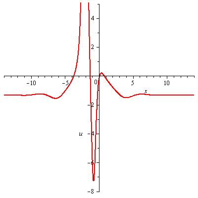
Figure 1: t=0

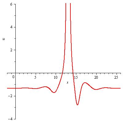
Figure 2: t=5

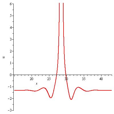
Figure 3: t=10

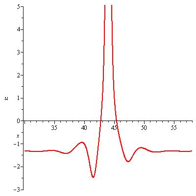
Figure 4: t=15

ii) $\alpha_{2}>0$, $\beta_{2}<0$. The functions $F(\xi)$ and $G(\eta)$ are

$$F(\xi)=\pm\.{i}\frac{\sqrt{\alpha_{2}}\mu_{2}k_{1}}{7\sqrt{-\beta_{2}}\mu_{1}k_{2}}\sinh\Big{(}\frac{\sqrt{-7\beta_{2}}k_{2}}{k_{1}}(\xi+A_{1})\Big{)},\quad G(\eta)=\pm\frac{\sqrt{\alpha_{2}}}{\sqrt{-\beta_{2}}}\sin(\sqrt{-\beta_{2}}(\eta+A_{2})),$$

and the solution is

$$u(x,t)=a_{0}+\frac{A}{B},$$ (2.14)

where

$$A = 384\rho\beta_{2}^{2}k_{2}^{2}-36\rho\beta_{2}k_{2}^{2}\sinh^{2}\Big{(}\frac{\sqrt{-7\beta_{2}}k_{2}}{k_{1}}(\xi+A_{1})\Big{)}-252\rho\beta_{2}k_{2}^{2}\sin^{2}(\sqrt{-\beta_{2}}(\eta+A_{2}))$$

$$\pm 168\.{i}\rho\beta_{2}k_{2}^{2}\sinh\Big{(}\frac{\sqrt{-7\beta_{2}}k_{2}}{k_{1}}(\xi+A_{1})\Big{)}\sin(\sqrt{-\beta_{2}}(\eta+A_{2})),$$

$$B = \zeta\Big{[}\.{i}\cosh\Big{(}\frac{\sqrt{-7\beta_{2}}k_{2}}{k_{1}}(\xi+A_{1})\Big{)}\mp\sqrt{7}\cos(\sqrt{-\beta_{2}}(\eta+A_{2}))\Big{]}^{2}.$$

If we separate the real and imaginary parts of the above solution we get,

$$\mathrm{Re}(u(x,t))=U(x,t)=a_{0}+\frac{B_{1}}{C_{1}},\quad\mathrm{Im}(u(x,t))=V(x,t)=\frac{B_{2}}{C_{1}},$$ (2.15)

where

$$B_{1} =12\rho\beta_{2}k_{2}^{2}[-14\cosh^{2}(\sigma_{1})+3\cosh^{4}(\sigma_{1})+147\cos^{4}(\sigma_{2})-42\cos^{2}(\sigma_{2})\cosh^{2}(\sigma_{1})$$ (2.16)

$$-28\sqrt{7}\sin(\sigma_{2})\cos(\sigma_{2})\sinh(\sigma_{1})\cosh(\sigma_{1})+98\cos^{2}(\sigma_{2})],$$

$$B_{2} =\pm 12\rho\beta_{2}k_{2}^{2}[-42\sqrt{7}\cosh(\sigma_{1})\cos^{3}(\sigma_{2})+14\sinh(\sigma_{1})\cosh^{2}(\sigma_{1})\sin(\sigma_{2})$$

$$-28\sqrt{7}\cosh(\sigma_{1})\cos(\sigma_{2})-98\sinh(\sigma_{1})\sin(\sigma_{2})\cos^{2}(\sigma_{2})+6\sqrt{7}\cosh^{3}(\sigma_{1})\cos(\sigma_{2})],$$

and

$$C_{1}=\zeta[\cosh^{2}(\sigma_{1})+7\cos^{2}(\sigma_{2})]^{2},$$ (2.17)

with $\displaystyle\sigma_{1}=\sqrt{-7\beta_{2}}k_{2}(\xi+A_{1})/k_{1}$, $\sigma_{2}=\sqrt{-\beta_{2}}(\eta+A_{2})$. Indeed, the couple $(U(x,t),V(x,t))$ is a novel non-singular solution of the coupled KdV equation (1.2).

For the following choice of the parameters; $\displaystyle\zeta=-6,\rho=1,\alpha_{2}=4,\beta_{2}=-1,\mu_{1}=1,\mu_{2}=1,k_{1}=2,k_{2}=1,a_{0}=1/6,A_{1}=A_{2}=0$, we have complexiton solution (2.15) where

$$\displaystyle B_{1} = 2[-14\cosh^{2}(\sqrt{7}(x+33t))+3\cosh^{4}(\sqrt{7}(x+33t))+98\cos^{2}(x+17t)$$

$$-28\sqrt{7}\sinh(\sqrt{7}(x+33t))\cosh(\sqrt{7}(x+33t))\sin(x+17t)\cos(x+17t)$$

$$-42\cos^{2}(x+17t)\cosh^{2}(\sqrt{7}(x+33t))+147\cos^{4}(x+17t)],$$

$$B_{2} = 4[-14\sqrt{7}\cosh(\sqrt{7}(x+33t))\cos(x+17t)-21\sqrt{7}\cosh(\sqrt{7}(x+33t))\cos^{3}(x+17t)$$

$$+7\cosh^{2}(\sqrt{7}(x+33t))\sinh(\sqrt{7}(x+33t))\sin(x+17t)$$

$$-49\sinh(\sqrt{7}(x+33t))\sin(x+17t)\cos^{2}(x+17t)$$

$$+3\sqrt{7}\cosh^{3}(\sqrt{7}(x+33t))\cos(x+17t)],$$

and

$$C_{1}=[\cosh^{2}(\sqrt{7}(x+33t))+7\cos^{2}(x+17t)]^{2}.$$

Graphs of the function $U(x,t)$ at some fixed times;

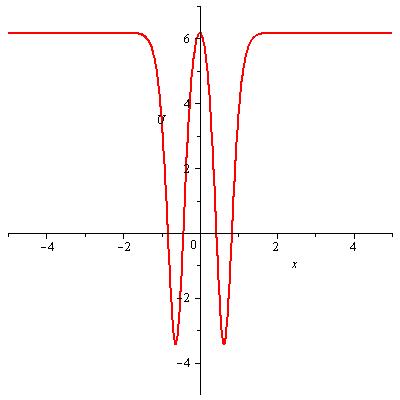
Figure 5: t=0

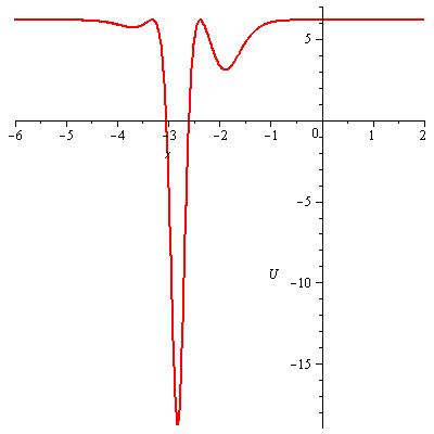
Figure 6: t=0.08

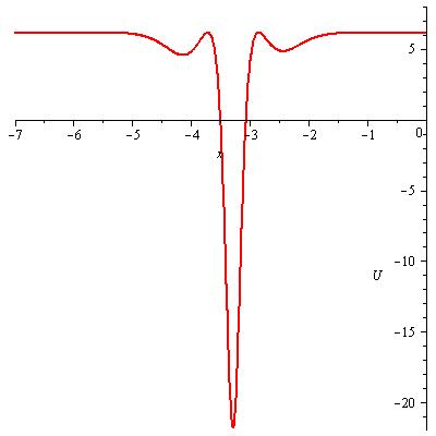
Figure 7: t=0.1

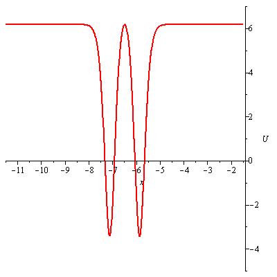
Figure 8: t=0.1963

And graphs of the function $V(x,t)$ are the followings.

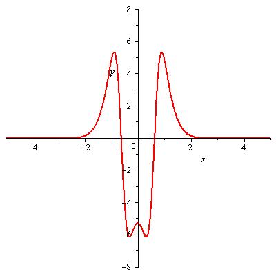
Figure 9: t=0

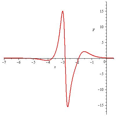
Figure 10: t=0.08

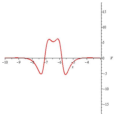
Figure 11: t=0.195

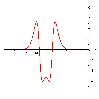
Figure 12: t=0.393

iii) $\alpha_{2}>0$, $\beta_{2}>0$. The functions $F(\xi)$ and $G(\eta)$ are

$$F(\xi)=\pm\.{i}\frac{\sqrt{\alpha_{2}}\mu_{2}k_{1}}{7\sqrt{\beta_{2}}\mu_{1}k_{2}}\sin\Big{(}\frac{\sqrt{7\beta_{2}}k_{2}}{k_{1}}(\xi+A_{1})\Big{)},\quad G(\eta)=\pm\frac{\sqrt{\alpha_{2}}}{\sqrt{\beta_{2}}}\sinh(\sqrt{\beta_{2}}(\eta+A_{2})),$$

and the solution is

$$u(x,t)=U(x,t)+\.{i}V(x,t),$$ (2.18)

where $\displaystyle U(x,t)=a_{0}+\frac{B_{1}}{C_{1}}$ and $\displaystyle V(x,t)=\frac{B_{2}}{C_{1}}$ with

$$B_{1} = 12\rho\beta_{2}k_{2}^{2}[-14\cos^{2}(\sigma_{1})+3\cos^{4}(\sigma_{1})+147\cosh^{4}(\sigma_{2})-42\cosh^{2}(\sigma_{2})\cos^{2}(\sigma_{1})$$

$$+28\sqrt{7}\sinh(\sigma_{2})\cosh(\sigma_{2})\sin(\sigma_{1})\cos(\sigma_{1})+98\cosh^{2}(\sigma_{2})],$$

$$B_{2} = \pm 12\rho\beta_{2}k_{2}^{2}[-42\sqrt{7}\cos(\sigma_{1})\cosh^{3}(\sigma_{2})-14\sin(\sigma_{1})\cos^{2}(\sigma_{1})\sinh(\sigma_{2})$$

$$-28\sqrt{7}\cos(\sigma_{1})\cosh(\sigma_{2})+98\sin(\sigma_{1})\sinh(\sigma_{2})\cosh^{2}(\sigma_{2})+6\sqrt{7}\cos^{3}(\sigma_{1})\cosh(\sigma_{2})],$$

and

$$C_{1}=\zeta[\cos^{2}(\sigma_{1})+7\cosh^{2}(\sigma_{2})]^{2},$$

with $\displaystyle\sigma_{1}=\sqrt{7\beta_{2}}k_{2}(\xi+A_{1})/k_{1}$, $\sigma_{2}=\sqrt{\beta_{2}}(\eta+A_{2})$. Hence, we obtain another new non-singular solution $(U(x,t),V(x,t))$ of the coupled KdV equation (1.2).

For a set of specific values and choice of signs; $\displaystyle\zeta=-6,\rho=1,\alpha_{2}=4,\beta_{2}=1,\mu_{1}=1,\mu_{2}=1,k_{1}=2,k_{2}=1,a_{0}=1/6,A_{1}=A_{2}=0$, we have complexiton solutions of the form (2.15) where

$$\displaystyle B_{1} = 2[14\cos^{2}(\sqrt{7}(x-31t))-3\cos^{4}(\sqrt{7}(x-31t))-98\cosh^{2}(x-15t)$$

$$-28\sqrt{7}\sin(\sqrt{7}(x-31t))\cos(\sqrt{7}(x-31t))\sinh(x-15t)\cosh(x-15t)$$

$$+42\cosh^{2}(x-15t)\cos^{2}(\sqrt{7}(x-31t))-147\cosh^{4}(x-15t)],$$

$$B_{2} = 4[14\sqrt{7}\cos(\sqrt{7}(x-31t))\cos(x-15t)+21\sqrt{7}\cos(\sqrt{7}(x-31t))\cosh^{3}(x-15t)$$

$$+7\cos^{2}(\sqrt{7}(x-31t))\sin(\sqrt{7}(x-31t))\sinh(x-15t)$$

$$-49\sin(\sqrt{7}(x-31t))\sinh(x-15t)\cosh^{2}(x-15t)$$

$$-3\sqrt{7}\cos^{3}(\sqrt{7}(x-31t))\cosh(x-15t)],$$

and

$$C_{1}=[\cos^{2}(\sqrt{7}(x-31t))+7\cosh^{2}(x-15t)]^{2}.$$

Let us illustrate the above solutions $U(x,t)$ and $V(x,t)$ at some fixed times. The graphs of $U(x,t)$ are

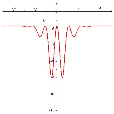
Figure 13: t=0

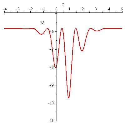
Figure 14: t=0.05

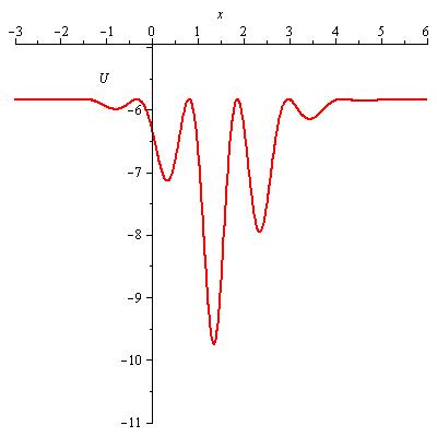
Figure 15: t=0.1

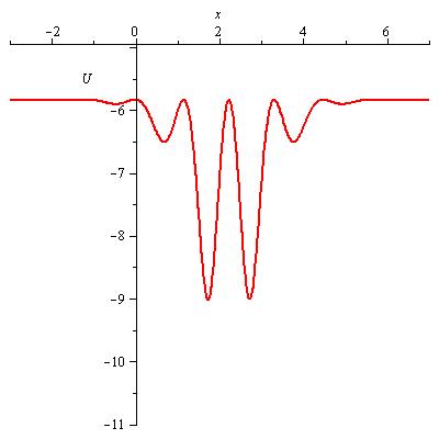
Figure 16: t=0.148

And graphs of the function $V(x,t)$ are the followings.

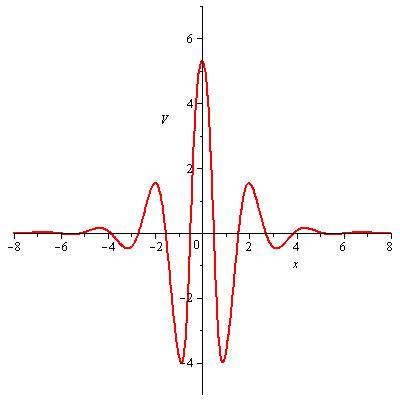
Figure 17: t=0

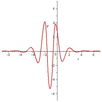
Figure 18: t=0.07

Figure 19: t=0.1

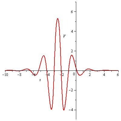
Figure 20: t=0.149

iv) $\alpha_{2}<0$, $\beta_{2}<0$. Here the functions $F(\xi)$ and $G(\eta)$ are

$$F(\xi)=\pm\frac{\sqrt{-\alpha_{2}}\mu_{2}k_{1}}{7\sqrt{-\beta_{2}}\mu_{1}k_{2}}\sinh\Big{(}\frac{\sqrt{-7\beta_{2}}k_{2}}{k_{1}}(\xi+A_{1})\Big{)},\quad G(\eta)=\pm\.{i}\frac{\sqrt{-\alpha_{2}}}{\sqrt{-\beta_{2}}}\cos(\sqrt{-\beta_{2}}(\eta+A_{2})),$$

and the solution is

$$u(x,t)=U(x,t)+\.{i}V(x,t),$$ (2.19)

where $\displaystyle U(x,t)=a_{0}+\frac{B_{1}}{C_{1}}$ and $\displaystyle V(x,t)=\frac{B_{2}}{C_{1}}$ with

$$B_{1} = 12\rho\beta_{2}k_{2}^{2}[-14\cosh^{2}(\sigma_{1})+3\cosh^{4}(\sigma_{1})+147\sin^{4}(\sigma_{2})-42\sin^{2}(\sigma_{2})\cosh^{2}(\sigma_{1})$$

$$+28\sqrt{7}\sin(\sigma_{2})\cos(\sigma_{2})\sinh(\sigma_{1})\cos(\sigma_{2})+98\sin^{2}(\sigma_{2})],$$

$$B_{2} = \pm 12\rho\beta_{2}k_{2}^{2}[-42\sqrt{7}\cosh(\sigma_{1})\sin^{3}(\sigma_{2})-14\sinh(\sigma_{1})\cosh^{2}(\sigma_{1})\cos(\sigma_{2})$$

$$-28\sqrt{7}\cosh(\sigma_{1})\sin(\sigma_{2})+98\sinh(\sigma_{1})\cos(\sigma_{2})\sin^{2}(\sigma_{2})+6\sqrt{7}\cosh^{3}(\sigma_{1})\sin(\sigma_{2})],$$

and

$$C_{1}=\zeta[\cosh^{2}(\sigma_{1})+7\sin^{2}(\sigma_{2})]^{2},$$

where $\displaystyle\sigma_{1}=\sqrt{-7\beta_{2}}k_{2}(\xi+A_{1})/k_{1}$, $\sigma_{2}=\sqrt{-\beta_{2}}(\eta+A_{2})$. The above solution is also a new non-singular solution $(U(x,t),V(x,t))$ of the coupled KdV equation (1.2).

Similar solutions can also be obtained with the following set of conditions:

Set 1:  $\gamma_{1}=\gamma_{2}=a_{1}=a_{2}=\kappa_{1}=\mu_{0}=0$, and

$$\displaystyle a_{3}=\frac{4\rho\mu_{1}^{2}\beta_{2}^{2}k_{2}^{4}}{3k_{1}^{2}\zeta},\quad a_{4}=\frac{8\rho\mu_{1}\mu_{2}k_{2}^{3}\beta_{2}^{2}}{k_{1}\zeta},\quad a_{5}=-\frac{4\rho\mu_{2}^{2}\beta_{2}^{2}k_{2}^{2}}{\zeta},\quad\kappa_{2}=\frac{32\rho k_{2}^{2}\mu_{2}^{2}\beta_{2}\alpha_{2}}{\zeta},$$

$$\alpha_{1}=-\frac{3\alpha_{2}\mu_{2}^{2}}{\mu_{1}^{2}},\quad\beta_{1}=-\frac{\beta_{2}k_{2}^{2}}{3k_{1}^{2}},\quad c_{1}=-\frac{4}{3}\rho\beta_{2}k_{2}^{2}+a_{0}\zeta,\quad c_{2}=-4\rho\beta_{2}k_{2}^{2}+a_{0}\zeta.$$

Set 2:  We have one more set of conditions; $\gamma_{1}=\gamma_{2}=a_{1}=a_{2}=\kappa_{1}=\mu_{0}=0$, and

$$\displaystyle a_{3}=-\frac{36\rho k_{2}^{4}\beta_{2}^{2}\mu_{1}^{2}}{k_{1}^{2}\zeta},\quad a_{4}=\frac{72\rho\mu_{1}\mu_{2}\beta_{2}^{2}k_{2}^{3}}{k_{1}\zeta},\quad a_{5}=\frac{12\rho\mu_{2}^{2}\beta_{2}^{2}k_{2}^{2}}{\zeta},\quad\kappa_{2}=\frac{32\rho k_{2}^{2}\mu_{2}^{2}\beta_{2}\alpha_{2}}{\zeta},$$

$$\alpha_{1}=-\frac{\alpha_{2}\mu_{2}^{2}}{3\mu_{1}^{2}},\quad\beta_{1}=-\frac{3\beta_{2}k_{2}^{2}}{k_{1}^{2}},\quad c_{1}=12\rho\beta_{2}k_{2}^{2}+a_{0}\zeta,\quad c_{2}=4\rho\beta_{2}k_{2}^{2}+a_{0}\zeta.$$

Case 2. Let $\gamma_{1}=\gamma_{2}=\mu_{0}=a_{1}=a_{2}=a_{3}=a_{5}=\kappa_{1}=0$,

$$a_{4}=\frac{24\rho\mu_{1}\mu_{2}\beta_{2}^{2}k_{2}^{3}}{k_{1}\zeta},\quad\kappa_{2}=\frac{24\rho\mu_{2}^{2}\beta_{2}k_{2}^{2}\alpha_{2}}{\zeta},\quad\alpha_{1}=-\frac{\alpha_{2}\mu_{2}^{2}}{\mu_{1}^{2}}$$

$$\beta_{1}=-\frac{\beta_{2}k_{2}^{2}}{k_{1}^{2}},\quad c_{1}=2\rho\beta_{2}k_{2}^{2}+a_{0}\zeta,\quad c_{2}=-2\rho\beta_{2}k_{2}^{2}+a_{0}\zeta.$$

i) $\alpha_{2}<0$, $\beta_{2}>0$. Similar to Case 1., the only case that we have real-valued solutions is when $\alpha_{2}<0$ and $\beta_{2}>0$. In this case, we obtain the functions $F(\xi)$ and $G(\eta)$ from (2.6) as

$$F(\xi)=\pm\frac{\sqrt{-\alpha_{2}}k_{1}\mu_{2}}{\sqrt{\beta_{2}}\mu_{1}k_{2}}\sin\Big{(}\frac{\sqrt{\beta_{2}}k_{2}}{k_{1}}(\xi+A_{1})\Big{)},\quad G(\eta)=\pm\frac{\sqrt{-\alpha_{2}}}{\sqrt{\beta_{2}}}\cosh(\sqrt{\beta_{2}}(\eta+A_{2})),$$

so the solution becomes

$$u(x,t)=a_{0}+\frac{-24\rho\beta_{2}k_{2}^{2}\pm 24\rho\beta_{2}k_{2}^{2}\sin\Big{(}\frac{\sqrt{\beta_{2}}k_{2}}{k_{1}}(\xi+A_{1})\Big{)}\cosh(\sqrt{\beta_{2}}(\eta+A_{2}))}{\zeta\Big{[}\cos\Big{(}\frac{\sqrt{\beta_{2}}k_{2}}{k_{1}}(\xi+A_{1})\Big{)}\pm\sinh(\sqrt{\beta_{2}}(\eta+A_{2}))\Big{]}^{2}},$$ (2.20)

where $\displaystyle\delta_{1}=24\rho\mu_{2}^{2}\beta_{2}k_{2}^{2}/\zeta$ and $A_{1}$, $A_{2}$ are arbitrary constants. Indeed, by some change of variables this solution can be reduced to the complexiton solution of the KdV equation in [17]-[19].

For the following choice of the parameters and signs;

$$\zeta=-6,\rho=1,\alpha_{2}=-4,\beta_{2}=\frac{1}{4},\mu_{1}=1,\mu_{2}=-1,k_{1}=-1,k_{2}=2,a_{0}=\frac{1}{6},A_{1}=A_{2}=0,$$

we get the solution

$$u(x,t)=\frac{1}{6}+\frac{4-4\sin(-x+t)\cosh(x+3t)}{[\cos(-x+t)-\sinh(x+3t)]^{2}}.$$ (2.21)

The graphs of this solution are given as follows:

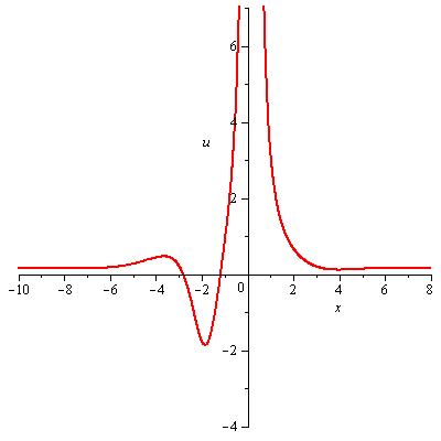
Figure 21: t=0

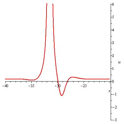
Figure 22: t=10

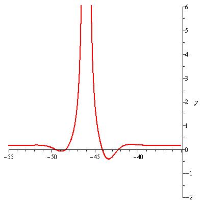
Figure 23: t=15

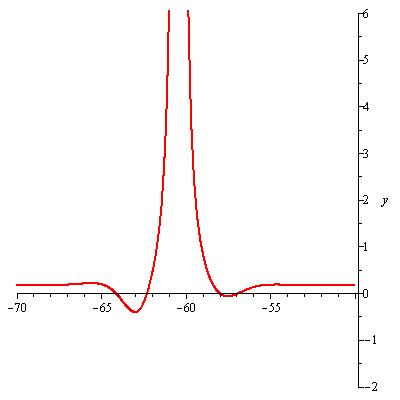
Figure 24: t=20

ii) $\alpha_{2}>0$, $\beta_{2}<0$. In this case, the functions $F(\xi)$ and $G(\eta)$ become

$$F(\xi)=\pm\.{i}\frac{\sqrt{\alpha_{2}}\mu_{2}k_{1}}{\sqrt{-\beta_{2}}\mu_{1}k_{2}}\sinh\Big{(}\frac{\sqrt{-\beta_{2}}k_{2}}{k_{1}}(\xi+A_{1})\Big{)},\quad G(\eta)=\pm\frac{\sqrt{\alpha_{2}}}{\sqrt{-\beta_{2}}}\sin(\sqrt{-\beta_{2}}(\eta+A_{2})),$$

and the solution is

$$u(x,t)=U(x,t)+\.{i}V(x,t),$$ (2.22)

where

$$U(x,t)=a_{0}+\frac{A}{C},\quad V(x,t)=\frac{B}{C},$$ (2.23)

where

$$A =a_{0}+24\rho\beta_{2}k_{2}^{2}[\cos^{2}(\sigma_{1})-\cosh^{2}(\sigma_{2})-2\sin(\sigma_{1})\cos(\sigma_{1})\sinh(\sigma_{2})\cosh(\sigma_{2})],$$ (2.24)

$$B =24\rho\beta_{2}k_{2}^{2}[\sin(\sigma_{1})\sinh(\sigma_{2})\cosh^{2}(\sigma_{2})-2\cos(\sigma_{1})\cosh(\sigma_{2})-\sinh(\sigma_{2})\sin(\sigma_{1})\cos^{2}(\sigma_{1})],$$

$$C =\zeta[\cosh^{2}(\sigma_{2})+\cos^{2}(\sigma_{1})]^{2},$$

with $\sigma_{1}=\sqrt{-\beta_{2}}(\eta+A_{2})$ and $\displaystyle\sigma_{2}=\sqrt{-\beta_{2}}k_{2}(\xi+A_{1})/k_{1}$, and $A_{1}$, $A_{2}$ are arbitrary constants.

For a set of specific values and choice of signs; $\displaystyle\zeta=-6,\rho=1,\alpha_{2}=4,\beta_{2}=-\frac{1}{4},\mu_{1}=1,\mu_{2}=-1,k_{1}=-1,k_{2}=2,a_{0}=1/6,A_{1}=A_{2}=0$, we have non-singular complexiton solutions of the form (2.23) where the terms $A$, $B$, and $C$ in (2.24) becomes

$$\displaystyle A = 4[\cos^{2}(-x+t)-\cosh^{2}(x+3t)+2\sinh(x+3t)\cosh(x+3t)\sin(-x+t)\cos(-x+t)],$$

$$B = 4[\sinh(x+3t)\sin(-x+t)\cos^{2}(-x+t)-\sin(-x+t)\sinh(x+3t)\cosh^{2}(x+3t)$$

$$-2\cos(-x+t)\cosh(x+3t)],$$

and

$$C=[\cosh^{2}(x+3t)+\cos^{2}(-x+t)]^{2}.$$

Firstly, let us present the graphs of the solution $U(x,t)$,

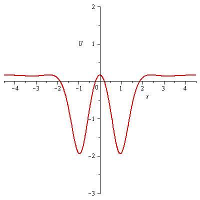
Figure 25: t=0

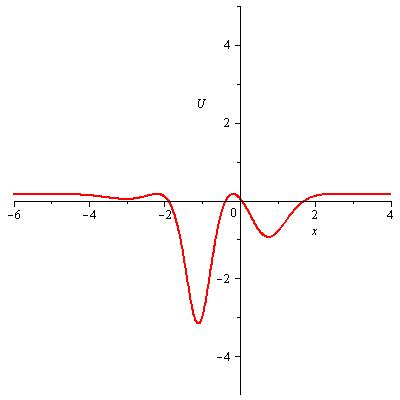
Figure 26: t=0.2

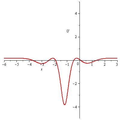
Figure 27: t=0.4

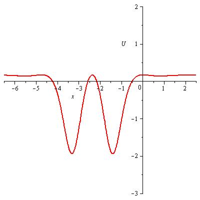
Figure 28: t=0.785

The graphs of the solution $V(x,t)$ are

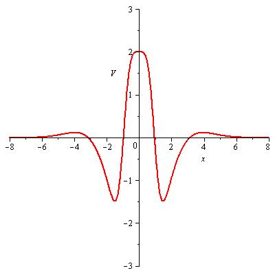
Figure 29: t=0

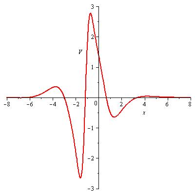
Figure 30: t=0.3

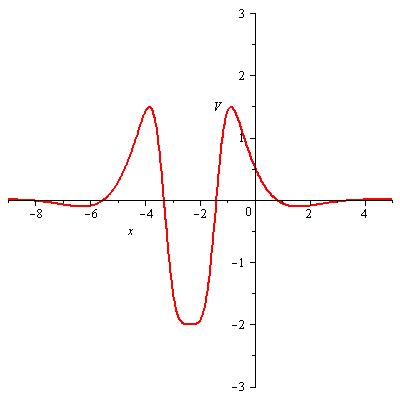
Figure 31: t=0.785

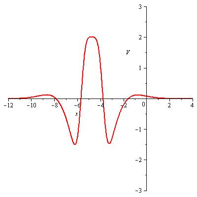
Figure 32: t=1.575

iii) $\alpha_{2}>0$, $\beta_{2}>0$. The functions $F(\xi)$ and $G(\eta)$ are

$$F(\xi)=\pm\.{i}\frac{\sqrt{\alpha_{2}}\mu_{2}k_{1}}{\sqrt{\beta_{2}}\mu_{1}k_{2}}\sin\Big{(}\frac{\sqrt{\beta_{2}}k_{2}}{k_{1}}(\xi+A_{1})\Big{)},\quad G(\eta)=\pm\frac{\sqrt{\alpha_{2}}}{\sqrt{\beta_{2}}}\sinh(\sqrt{\beta_{2}}(\eta+A_{2})),$$

and the solution is

$$u(x,t)=U(x,t)+\.{i}V(x,t).$$ (2.25)

Here we have

$$U(x,t)=a_{0}+\frac{A}{C},\quad V(x,t)=\frac{B}{C},$$ (2.26)

where

$$A =a_{0}+24\rho\beta_{2}k_{2}^{2}[\cosh^{2}(\sigma_{1})-\cos^{2}(\sigma_{2})+2\sinh(\sigma_{1})\cosh(\sigma_{1})\sin(\sigma_{2})\cos(\sigma_{2})],$$ (2.27)

$$B =\pm 24\rho\beta_{2}k_{2}^{2}[\sin(\sigma_{2})\sinh(\sigma_{1})\cosh^{2}(\sigma_{1})-\sinh(\sigma_{1})\sin(\sigma_{2})\cos^{2}(\sigma_{2})-2\cosh(\sigma_{1})\cos(\sigma_{2})],$$

$$C =\zeta[\cosh^{2}(\sigma_{1})+\cos^{2}(\sigma_{2})]^{2},$$

with $\sigma_{1}=\sqrt{\beta_{2}}(\eta+A_{2})$ and $\displaystyle\sigma_{2}=\sqrt{\beta_{2}}k_{2}(\xi+A_{1})/k_{1}$, and $A_{1}$, $A_{2}$ are arbitrary constants. The couple $(U(x,t),V(x,t))$ is another solution of (1.2).

iv) $\alpha_{2}<0$, $\beta_{2}<0$. The functions $F(\xi)$ and $G(\eta)$ are

$$F(\xi)=\pm\frac{\sqrt{-\alpha_{2}}\mu_{2}k_{1}}{\sqrt{-\beta_{2}}\mu_{1}k_{2}}\sinh\Big{(}\frac{\sqrt{-\beta_{2}}k_{2}}{k_{1}}(\xi+A_{1})\Big{)},\quad G(\eta)=\pm\.{i}\frac{\sqrt{-\alpha_{2}}}{\sqrt{-\beta_{2}}}\cos(\sqrt{-\beta_{2}}(\eta+A_{2})),$$

and the solution is

$$u(x,t)=U(x,t)+\.{i}V(x,t),$$ (2.28)

where

$$U(x,t)=a_{0}+\frac{A}{C},\quad V(x,t)=\frac{B}{C},$$ (2.29)

with

$$A =a_{0}+24\rho\beta_{2}k_{2}^{2}[\sin^{2}(\sigma_{1})-\cosh^{2}(\sigma_{2})+2\sin(\sigma_{1})\cos(\sigma_{1})\sinh(\sigma_{2})\cosh(\sigma_{2})],$$ (2.30)

$$B =\pm 24\rho\beta_{2}k_{2}^{2}[\sinh(\sigma_{2})\cos(\sigma_{1})\sin^{2}(\sigma_{1})-\cos(\sigma_{1})\sinh(\sigma_{2})\cosh^{2}(\sigma_{2})-2\sin(\sigma_{1})\cosh(\sigma_{2})],$$

$$C =\zeta[\cosh^{2}(\sigma_{2})+\sin^{2}(\sigma_{1})]^{2},$$

where $\sigma_{1}=\sqrt{-\beta_{2}}(\eta+A_{2})$ and $\displaystyle\sigma_{2}=\sqrt{-\beta_{2}}k_{2}(\xi+A_{1})/k_{1}$, and $A_{1}$, $A_{2}$ are arbitrary constants. The couple $(U(x,t),V(x,t))$ is a solution of (1.2).

3 Asymptotic Behaviors of the Solutions

Both of the complexiton solutions obtained in Case 1. that is the solution (2.10) with (2.11) and the solution (2.20) found in Case 2. are singular solutions. For any parameters in these solutions, obviously the denominators of them vanish at some points at a fixed time. The solution (2.10) with (2.11) approaches to a constant $\displaystyle a_{0}+252\rho k_{2}^{2}\beta_{2}/7\zeta$ as $x\rightarrow\pm\infty$ and similarly as $t\rightarrow\pm\infty$. Other solution (2.20) obtained in Case 2. approaches to $a_{0}$ as $x\rightarrow\pm\infty$ and as $t\rightarrow\pm\infty$. Even approaching to a constant is one of the main properties of solitary wave solutions, it is clear that these solutions are not solitary wave solutions since they have blowing-ups which can also be realized through the graphs given. The graphs also show that because of the trigonometric functions both of the solutions tend to be periodic but by hyperbolic functions their periodicity fades away.

Other solutions that are complex-valued solutions of the KdV equation give real-valued non-singular solutions of the coupled KdV equation (1.2). For instance, in Case 1. we get the solution (2.15) as a couple $(U(x,t),V(x,t))$ with (2.16) and (2.17). Notice that while the solution $U(x,t)$ approaches to $a_{0}+36\rho\beta_{2}k_{2}^{2}/\zeta$ as $x\rightarrow\pm\infty$, and $t\rightarrow\pm\infty$, the solution $V(x,t)$ approaches to zero. If the graphs of the solutions $U(x,t)$ and $V(x,t)$ are analyzed, one can realize that the waves defined by the solutions change their forms as time changes but at some point they return to their original shapes.

4 Conclusion

We presented a new approach to double-sub equation method which is a practical and an appropriate method for symbolic computation in MAPLE or Mathematica to explore novel solutions of nonlinear partial differential equations. Specifically, we applied this method on the $(1+1)$-dimensional KdV equation and obtained periodic and solitary wave solutions, and notably complexiton solutions depending on two independent variables which are novel solutions to the best of our knowledge. In addition to that application of this approach produced new complexiton solutions of the coupled KdV equation.

This method can be applied to many other nonlinear integrable and non-integrable equations. In this study, we used a $(1+1)$-dimensional equation but by introducing an additional function and a first order ODE satisfied by this new function we can also apply this method to $(2+1)$-dimensional or even higher order partial differential equations. Indeed, it is worth to generalize this approach and study on a unification of many of the solution methods in the literature which may also produce interesting solutions of well-known partial differential equations.

5 Acknowledgment

This work is partially supported by the Scientific and Technological Research Council of Turkey (TÜBİTAK).