Lattice Model for water-solute mixtures.

Abstract

A lattice model for the study of mixtures of associating liquids is proposed. Solvent and solute are modeled by adapting the associating lattice gas (ALG) model. The nature of interaction solute/solvent is controlled by tuning the energy interactions between the patches of ALG model. We have studied three set of parameters, resulting on, hydrophilic, inert and hydrophobic interactions. Extensive Monte Carlo simulations were carried out and the behavior of pure components and the excess properties of the mixtures have been studied. The pure components: water (solvent) and solute, have quite similar phase diagrams, presenting: gas, low density liquid, and high density liquid phases. In the case of solute, the regions of coexistence are substantially reduced when compared with both the water and the standard ALG models. A numerical procedure has been developed in order to attain series of results at constant pressure from simulations of the lattice gas model in the grand canonical ensemble. The excess properties of the mixtures: volume and enthalpy as the function of the solute fraction have been studied for different interaction parameters of the model. Our model is able to reproduce qualitatively well the excess volume and enthalpy for different aqueous solutions. For the hydrophilic case, we show that the model is able to reproduce the excess volume and enthalpy of mixtures of small alcohols and amines. The inert case reproduces the behavior of large alcohols such as, propanol, butanol and pentanol. For last case (hydrophobic), the excess properties reproduce the behavior of ionic liquids in aqueous solution.

I Introduction

Mixtures of water and organic solutes are of fundamental importance for understanding biological and chemical processes as well as transport properties of fluids. Even though the simplicity, of these solutions some of them show a complex behavior of their thermodynamic and structural properties Evans1945 . For example, close to the ambient conditions, around $T=298.15\>K$, $p=1{\rm bar}$, the excess volume in binary mixtures of water and alcohols Marongiu1984 ; Pattel1985 ; Ben-Naim2008 ; Sha2016 ; Ott1993 and of water and alkanolamines Hepler1994 ; Stec2014 is negative and it exhibits a minimum as the fraction of the solute is increased. In the case of water-ionic liquids, however, the excess volume depend on the hydrophobicity of the solute. Simulation results suggest that for hydrophilic solutes as the 1,3-dimethylimidazolium chloride the excess volume has a minimum as in the case of the alcohols, whereas for the case of more hydrophobic liquids as the 1,3-dimethylimidazolium hexafluorophosphate the excess volume is positive Henke2003 .

The excess enthalpy of the aqueous organic mixtures also show a distinct behavior. While the mixtures of water with small alcohol molecules as methanol Marongiu1984 ; Randzio1986 ; Tomasziewicz1986 and ethanol Marongiu1984 ; Ott1986 exhibit a negative excess enthalpy, the mixtures of water with large alcohol molecules as propanol and butanol isomers show a positive excess enthalpy Marongiu1984 . Similarly to the small alcohol-water mixtures the excess enthalpy for the water-alkanolamine solutions also show a minimum Mundhwa2007 . In the case of ionic liquids the excess enthalpy also show two types of behavior. For the less hydrophobic ionic liquids in which the excess volume is negative, the excess enthalpy is negative and shows a minimum at the same solute fraction of the minimum of the excess volume. For the hydrophobic ionic liquids the excess enthalpy is positive and shows a maximum for the same fraction of the solute of the maximum of the excess volume Miaja2009 ; Vatascin2015 .

The excess isobaric specific heat for the methanol at ambient conditions increases with the fraction of the solute and exhibits a maximum value around the solute concentration $x_{2}=0.16$ Benson1980 ; Benson1982 . The excess free energy presents a harmonic dependence on the methanol fraction Butler1933 and the excess entropy of mixing, differently from the ideal mixtures McQuarrie1975 , assumes negative values and decrease its value as the increasing methanol concentrations Lama1965 . In the case of the ionic liquids the constant pressure heat capacity also shows an oscillatory behavior but the peak occurs at higher concentrations of the solute $x_{2}=0.3$ Miaja2009 ; Vatascin2015 .

The description of this complex behavior of the organic solutes in water in can be made, in principle, in the framework of the Frank and Evans Evans1945 iceberg theory. These authors proposed that water is able to form microscopic icebergs around solute molecules depending on their size and the water-solute interactions. Recent experiments Dixit2002 using neutron diffraction support Frank and Evans Evans1945 scenario for the methanol. The diffraction of a concentrated alcohol-water mixture ($x_{2}=0.70$) suggests that at these conditions most of the water molecules ($\sim 87\%$) are organized in water clusters bridging methanol hydroxyl groups through hydrogen bonds. In the same direction an experimental result from X-ray emission spectroscopy for an equimolar mixture of methanol and water carried out by Guo et.al. Guo2003 suggests that in the mixture the hydrogen bonding network of the pure components would persist to a large extent, with some water molecules acting as bridges between methanol chains. Consistent with these results, recent experimental work for the methanol Dixit2002 ; Guo2003 suggests that the negative excess the entropy of mixing arises due to a relatively small degree of the interconnection between the hydrogen bonding networks of the different components rather than from a water restructuring Dixit2002 .

Motivated by these experimental results and by the huge number of applications, water-methanol mixtures have been intensively studied by computer simulations. In these simulations, water molecules are represented by one of well known classical models SPC$/$E Berendsen1987 , ST4 HeadGordon1993 , TIP5P Jorgensen2000 and methanol molecules are frequently modeled by OPLS force field Jorgensen1996 . Using Molecular Dynamics simulation, Bako et.al. Bako2008 found that on increasing the methanol fraction in the mixture, water essentially maintains its tetrahedral structure, whereas the number of hydrogen-bonds is substantially reduced. Allison et.al. Allison2005 showed that not only the number hydrogen-bonds decreases, but the water molecules become eventually distributed in rings and clusters in accordance with the experimental results Dixit2002 . Analyzing the spatial distribution function of the water, Laaksonen et.al. Laaksonen1997 observed that the system is highly structured around the hydroxyl groups and that the methanol molecules are solvated by water molecules, in accordance with well known iceberg theory Evans1945 .

In addition to the atomistic approaches, water-methanol mixture has been modeled by continuous potentials in which the water is represented by a spherical symmetric two length scale potential while the methanol is represented by a dimer in which the methyl group is characterized by a hard sphere and the hydroxyl is a water-like group hus2014 ; zhiqiang2012 . Numerical simulations for this system displays good qualitative agreement with the response functions for different temperatures hus2014 ; zhiqiang2012 but fails to produce the heat capacity behavior and does not provide the structural network observed in experiments and predicted by the iceberg theory.

Due to the variety and complexity of the ionic liquids, very few theoretical studies have been made for analyzing the ionic liquids aqueous solutions. For example, there is no clear picture explaining why the excess volume of some ionic liquids is negative while for others is positive. In addition, it is not clear why for large alcohols the excess enthalpy is positive while for the methanol is negative. The explanation for these different behaviors both in the alcohols and in the ionic liquids might rely in the disruption of the iceberg theory as the solute is large of hydrophobic. In order to test this idea, here we explore how the excess properties of the water-solute mixture is affected by the change of the water-solute interaction from attractive to repulsive. In order to allow for the water to form a structure not present in the continuous effective potentials, our model exhibits a tetrahedral structure.

In this work the water and the solute are modeled following the associating lattice gas model (ALG) Girardi2007 ; Szortyka2010 ; Szortyka2012 scheme. The two molecules are specified by adapting the hydrogen bond and the attractive interactions for each molecule. The excess volume and enthalpy are computed for various types of water-solute interactions.

The remaining of the paper goes as follows. In the Section II the models for water, solute and mixture are outlined and the ground state behavior is presented. The technical details about the calculations of ground state are presented in the Appendix A. In the Section III the computational methods are described and the technical aspects can be found in Appendix B and C. In the Section IV results are presented. Section V ends the paper with the conclusions.

II Model

We consider three systems: pure water, pure solute and water-solute mixture. In the three cases the system is defined on a body-centered cubic (BCC) lattice. Sites on the lattice can be either empty or occupied by a water or by a solute molecule. Particles representing both water and solute molecules carry four arms that point to four of the nearest neighbor (NN) sites on the BCC lattice as illustrated by the figure 1. The interactions between NN molecules are described in the framework of the lattice patchy models Almarza2012a . The particles carry eight patches (four of them corresponding to the arms in the ALG model), and each of the patches points to one of the NN sites in the BCC lattice as illustrated in the figure 1. The water molecules have two patches of the type $A$ (acceptors), two patches of the type $B$(donors) and four patches of the type $D$ (which do not participate in bonding interactions). Since the patches of the types $A$ and $B$ participate in the hydrogen bonding, a water molecule can participate in up to four hydrogen bonds. The structure of the solute is similar to the structure of the water, but it has only one patch of type $A$, the other patch $A$ is replaced by a patch of the type $C$ that represents the anisotropic group which makes water and the solute different. In the case in which the solute is the methanol $C$ is the methyl group while for other alcohols and ionic liquids it does represent larger chains.

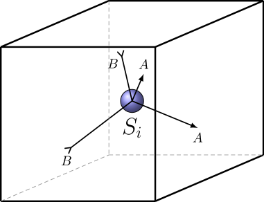
Figure 1: Representation of lattice for pure components. The blue sphere represents the water and the patches $A$ and $B$ represent the acceptors and donors arms respectively. The red sphere represent the solute particle and the arms $A$ and $B$ represent the acceptor and donors, and the patch $C$ represents the anisotropic group

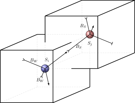
Figure 2: Representation of lattice. $S_{i}$ and $S_{j}$ represent particle on its respective positions $i$ and $j$. Blue sphere represent a water and red, a solute particle. $B_{W}$ and $B_{S}$ represent the patches B of water and solute respectively. The patch $D$ is not represented here for the clarity of the image.

The distinction between patches implies $12$ possible orientations for the water molecules and $24$ possible orientations for the solute molecules.

The potential energy is defined as a sum of interactions between pairs of particles located at sites which are NN on the BCC lattice. The interaction between particles $i$ and $j$, which are NN, only depends on the type of patch of particle $i$ that points to particle $j$, and on the type of patch of particle $j$ that points to particle $i$. The values of the interaction as a function of the types of the two interacting patches are summarized in the Table 1. The interaction between occupied neighbor sites is repulsive with an increase of energy by $\epsilon_{ij}=\epsilon$ with the exception of three cases. For patch-patch interaction of type $A-B$ the energy interaction is taken as: $\epsilon_{ij}=-\epsilon$. If the interaction is of type $B-C$, with the $B$ patch belonging to a solute molecule there is also an attractive interaction $\epsilon_{ij}=-\lambda_{S}\epsilon$ (with $\lambda_{S}>0)$, whereas if the patch $B$ belongs to a water molecule the interaction energy is given by $\epsilon_{ij}=-\lambda_{W}\epsilon$.

We have considered $\lambda_{S}=0.25$, and three cases for the $B$-$C$ water-solute interaction: attraction with $\lambda_{W}=\lambda_{S}$, non-interacting with $\lambda_{W}=0$ and repulsion with $\lambda_{W}<0$. The first case represents systems dominated by the water-solute attraction. This is the case of the methanol in which it is assumed that the methyl group shows a small but attractive interaction with the water. This also represents the ionic liquids in which the anions groups are hydrophilic and the cationic chains are not too long Freire2007 ; Ranke2009 . The second case represents alcohols with larger non-polar alkyl substituents Marongiu1984 . The third case represents the ionic liquids in which the combination of the anions and cations lead to an hydrophobic interaction Freire2007 ; Ranke2009 . Due to the simplicity of our model solute, size and hydrophobicity effects are not taken into account independently, but both are considered through the $\lambda_{W}$ parameter.

$p(S)$		D		A		BW		BS		C
D		$\epsilon$		$\epsilon$		$\epsilon$		$\epsilon$		$\epsilon$
A		$\epsilon$		$\epsilon$		$-\epsilon$		$-\epsilon$		$\epsilon$
BW		$\epsilon$		$-\epsilon$		$\epsilon$		$\epsilon$		$-\lambda_{W}\epsilon$
BS		$\epsilon$		$-\epsilon$		$\epsilon$		$\epsilon$		$-\lambda_{S}\epsilon$
C		$\epsilon$		$\epsilon$		$-\lambda_{W}\epsilon$		$-\lambda_{S}\epsilon$		$\epsilon$

Table 1: Interactions between NN particles of the same type (solute or water). The interaction depends on the patches of both particles involved in the interparticle bond. The interaction between patches of type C and B depends on the type of molecule: water (W) or solute (S) that provides the patch B. We consider $0<\lambda_{S}\leq 1$; and $\epsilon>0$. Patches of types A, B, and C correspond to the four arms of the standard ALG model.

At zero temperature for the cases of the pure water and the pure solute systems three possible thermodynamic phases can appear in the model: For low values of the chemical potential, $\mu$, the stable phase is the empty lattice representing the gas phase at reduced density, $\rho^{*}=N/N_{L}=0$, with $N$ being the number of particles (occupied sites) and $N_{L}$ the number of sites of the lattice. Increasing $\mu$ a low density liquid phase (LDL) appears Girardi2007 ; Buzano2008 ; Szortyka2010 ; Szortyka2012 , where half of the sites of the lattice are occupied by particles ($\rho^{*}=1/2$). These sites are those belonging to one of the diamond sublattices Almarza2011b that can be defined on the BCC lattice. Every patch of the type $A$ is pointing to a patch of the type $B$, and vice versa. In the case of water only pair interactions $AB$ occur. In the case of the solute both $AB$ and $CB$ interactions occur. At higher values of the chemical potential, the stable phase is the high density liquid (HDL), where all the sites are occupied, and as for the LDL phase, in the case of water, every patch of type $A$ is bonded to a patch of type $B$ and vice versa. In the case of the solute every patch of type $A$ is bonded to a patch of type $B$ and every patch of type $C$ is bounded to a patch of type $B$. The modification of the ALG model by considering different types of arms introduce, at zero temperature, a residual entropy per particle $s_{0}$, that in thermodynamic limit can be written as, $s_{0}=k_{B}\lim_{N\to\infty}\left[N^{-1}\ln{Q_{0}(N)}\right]$, where $k_{B}$ is Boltzmann’s constant, and $Q_{0}(N)$ is the number of configurations of the system, in which every patch of type B is interacting with a patch of type A (or C), and every patch of type A (or C) is interacting with a patch of type B. Using Monte Carlo (MC) simulations and thermodynamic integration techniques AllenTildesleyBook ; FrenkelSmitBook we have obtained the values of residual entropy for the water ($s^{\rm(W)}_{0}/k_{B}=0.41041\pm 0.00002$) and solute ($s_{0}^{\rm(S)}/k_{B}=1.10356\pm 0.00002$) models. For more details about the computation of residual entropies, see Appendix A.

From the values of residual entropy we can study the system in ground state. The Grand Canonical thermodynamic potential can be written as:

$$\Phi\equiv-pV=U-TS-\mu N,$$ (1)

where $U$ is the internal energy, $S$ is the entropy, and $N$ the number of particles (occupied positions). In the Ground State, the stable phase for a given value of $\mu$ is the one with the minimum value of $\Phi$. Considering the description of the ordered phases explained above, for the water model $\Phi$ take the values (for $T\rightarrow 0$):

$$\begin{array}[]{llllr}\Phi^{\rm(W)}_{G}(V,\mu)/V^{*}&=&0&&(\rho^{*}=0);\\ \Phi^{\rm(W)}_{LDL}(V,\mu)/V^{*}&=&-\epsilon-Ts^{\rm(W)}_{0}/2-\mu/2;&&(\rho^{*}=1/2);\\ \Phi^{\rm(W)}_{HDL}(V,\mu)/V^{*}&=&-Ts^{\rm(W)}_{0}-\mu;&&(\rho^{*}=1)\end{array}$$ (2)

with $V^{*}$ being the reduced volume (equal to the number of sites). Imposing that in coexistence the $\Phi^{\rm(W)}_{G}=\Phi^{\rm(W)}_{LDL}$ and $\Phi^{\rm(W)}_{LDL}=\Phi^{\rm(W)}_{HDL}$ we obtain the values of the chemical potential and the pressure, at the transitions in the limit of low temperatures

$$\begin{array}[]{lll}\mu=-2\epsilon-Ts_{0}^{\textrm{(W)}},&\quad pw_{0}/\epsilon=0,&\quad\textrm{G-LDL water}\\ \mu=2\epsilon-Ts_{0}^{\textrm{(W)}},&\quad pw_{0}/\epsilon=2,&\quad\textrm{LDL-HDL water};\end{array}$$ (3)

where the factor $w_{0}=V/N_{L}$ correspond to the volume per site. For the case of pure solute the thermodynamic potential $\Phi$ of the different phases as $T\rightarrow 0$ is given by

$$\begin{array}[]{llllr}\Phi_{G}^{\rm(S)}(V,\mu)/V^{*}&=&0;&&(\rho=0);\\ \Phi_{LDL}^{\rm(S)}(V,\mu)/V^{*}&=&-(1+\lambda_{S})\epsilon/2-Ts_{0}^{\textrm{(S)}}/2-\mu/2;&&(\rho=1/2);\\ \Phi_{HDL}^{\rm(S)}(V,\mu)/V^{*}&=&(1-\lambda_{S})\epsilon-Ts_{0}^{\textrm{(S)}}-\mu;&&(\rho=1),\end{array}$$ (4)

and for the phase equilibria at low temperature we get:

$$\begin{array}[]{lllll}\mu=-(1+\lambda_{S})\epsilon-Ts_{0}^{\textrm{(S)}},&&pw_{0}/\epsilon=0,&&\textrm{G-LDL solute},\\ \mu=(3-\lambda_{S})\epsilon-Ts_{0}^{\textrm{(S)}},&&pw_{0}/\epsilon=2,&&\textrm{LDL-HDL solute}\end{array}$$ (5)

All the relevant quantities will be expressed in reduced units, such as:

$$\mu^{*}=\dfrac{\mu}{\epsilon}\quad,\quad T^{*}=\dfrac{k_{B}T}{\epsilon}\quad,\quad c_{V}^{*}=\dfrac{c_{V}}{k_{B}},\quad p^{*}=\dfrac{pw_{0}}{\epsilon},\quad s^{*}=\dfrac{s}{k_{B}}$$ (6)

III Simulation and Numerical Details

In order to obtain the phase diagrams and compute the thermodynamic and structural properties of one-component systems, we have performed MC simulations in the grand canonical ensemble (GCE) for system sizes $512\leq N_{L}\leq 65536$ where $N_{L}=2L^{3}$. The simulations have used $\sim 8\times 10^{6}$ MC sweeps for equilibration and $\sim 4\times 10^{6}$ sweeps for evaluating the relevant quantities. Each MC sweep is defined as $N_{L}$ one-site attempts to generate a new configuration. Each attempt is carried out as follows: i) A site $i$ on the lattice is chosen at random; this site can adopt $n_{s}$ possible states, $S_{i}=0,1,2\cdots,n_{s}-1$ ($n_{s}=13$ for pure water; $n_{s}=25$ for pure solute, and $n_{s}=37$ for the mixtures); $S_{i}=0$ represents an empty site, and the remaining values stand for the different species that can occupy the site and their respective orientations. ii) For the selected site, one of its possible $n_{s}$ states is selected at random, with probabilities given by:

$$P(S_{i})\propto\exp\left[-\frac{U_{i}(S_{i})-\mu(S_{i})}{k_{B}T}\right],\hskip 28.45274ptS_{i}=0,1,2,\cdots,n_{s};$$ (7)

where $U_{i}(S_{i})$ contains the potential energy interactions between site $i$ at state $S_{i}$ with its NN, and $\mu(S_{i})$ is the chemical potential of the component associated with state $S_{i}$. Notice that for an empty site $S_{i}=0$, both $U_{i}(S_{i})$ and $\mu(S_{i})$ are zero, and that for $S_{i}\neq 0$, the value of $U_{i}$ depends on the states of the sites which are NN of $i$.

We have combined the one-site sampling procedure with different advanced techniques in order to enhance the simulation efficiency: In the regions close to continuous transitions, where critical slowing down may be present LandauBinderBook , we have made use of the Parallel Tempering (PT) methodSwendsen1986a ; Earl2005a . The Gibbs-Duhem integration Kofke1993 technique adapted for working in the GCE Almarza2011b ; Almarza2012a was employed in the location of the discontinuous phase transitions of the system. In order to study the excess properties of the mixtures as functions of the pressure and temperature we have developed methods to build up isobars for one-component systems (See Appendix B), and lines at constant pressure and temperature with varying composition for the binary mixtures (See Appendix C).

IV Numerical Results

IV.1 The phase diagram for pure components

The chemical potential $vs$. temperature phase diagrams are shown in the Fig. 3 for the pure water and for the pure solute. Three different phases, G, LDL, and HDL appear, as expected. At low temperature, there are two, G-LDL and LDL-HDL first-order transitions. The first order LDL-HDL transition finishes, both for water and solute, in a liquid-liquid tricritical point (LLTCP). The LLTCPs occur at $T^{*}_{tc}\simeq 0.59$ and $\mu^{*}_{tc}\simeq 1.67$ for water and at $T^{*}_{tc}=0.25$ $\mu^{*}_{tc}=2.42$ the solute. Above $T_{tc}$ the LDL-HDL transition becomes continuous and defines the $\lambda-$line (See Fig. 3). At high temperature, it appears a continuous transition between G and HDL phases ($\tau-$line in Fig. 3).

The coexistence line between the G and LDL phases for water extends up to a bicritical point (LGBCP) LavisBellBook located at $T_{bc}^{*}\simeq 1.00$ and $\mu_{bc}^{*}\simeq-0.22$. At this LGBCP the G-LDL transition meets the lines for the critical G-HDL ($\tau-$line) and LDL-HDL ($\lambda-$line) transitions. In the case of solute, the G-LDL first order transition meets the $\lambda$-line at an end point located at $T_{t}^{*}\simeq 0.74$, $\mu_{t}^{*}\simeq 0.86$. Above this temperature there is a G-HDL first order transition up to a tricritical point (LGTCP) located at $T_{tc}^{\prime*}\simeq 0.85$, $\mu_{tc}^{\prime*}=0.84$. Above this temperature the G-HDL transition becomes continues and defines the $\tau$-line.

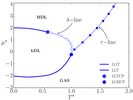
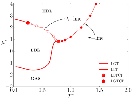
Figure 3: Reduced chemical potential versus reduced temperature phase diagram for (a) pure water (b) pure solute. Solid thick lines represent first-order phase transitions, liquid-gas (LGT) and liquid-liquid (LLT). Thin lines represent continuous (second-order) transition, the empty circles show the $\lambda-$line and the filled circles are the $\tau-$line. The big patterned circles represent the multi-critical points of the model. (See the text for details).

The continuous $\tau$ and $\lambda$ transitions, illustrated in the figure 3 are represented by thin lines and circles. The values of the temperatures and chemical potentials for the critical lines were obtained by computing appropriated order parameters and their associated moments or cumulants.

In the case of the $\lambda$ line, the $\theta_{\lambda}$ order parameter is defined as follows. The system is divided into eight sublattices Szortyka2010 . The figure 4 illustrates the behavior of the eight sublattices as a function of the temperature at the $\lambda$-line. As the temperature is decreased four sublattices become full while other four stay empty. Then, from the density of these sublattices, the order parameter is defined by

$$\theta_{\lambda}=\dfrac{2}{V}\left[\sum_{i=1}^{\rm full}\rho_{i}-\sum_{j=1}^{\rm empty}\rho_{j}\right],$$ (8)

where the index $i$ runs over the four sublattices which become full at the LDL phase while the subindex $j$ runs over the four sublattices which remain empty at the LDL phase. The figure 4 illustrates the value of this order parameter as a function of the temperature for fixed chemical potentials for both the pure water and the pure solute cases showing the transition from all the sublattices equally populated to a preferential occupation in four sublattices.

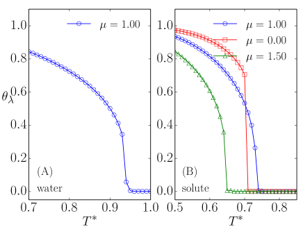
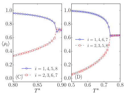
Figure 4: Order parameter $\theta_{t}$ versus reduced temperature for (A) water and (B) solute for various chemical potentials. Average density of the empty (red) and full (blue) sublattices for (C) water and for (D) the solute.

This transition can also be described by taking into account that for the ALG model there are four possible realizations of the LDL structure (with diamond structure) on the BCC lattice. The occupancy of the sites and orientations of the arms (patches of types A, B and C) is well defined for each LDL realization. Taking into account the orientation of the occupied sites on a given configuration, we can compute the number of particles in the system compatible with each of the four LDL realizations. Let $n_{i}$, with $i=1,2,3,4$ be those numbers. From each configuration, we can sort the $n_{i}$ values so that $n_{a}\geq n_{b}\geq n_{c}\geq n_{d}$, and compute their corresponding densitie s $\rho_{a}=n_{a}/N_{L},\rho_{b}=n_{b}/N_{L}\cdots$. In the thermodynamic limit ($N_{L}\rightarrow\infty$), we expect for the G phase: $\rho_{a}\simeq\rho_{b}\simeq\rho_{c}\simeq\rho_{d}\simeq\rho/4$. For the HDL phase $\rho_{a}\simeq\rho_{b}\gg\rho_{c}\simeq\rho_{d}$, and finally for the LDL phase $\rho_{a}\gg\rho_{b}$. Accordingly the presence of the LDL phase can be detected by an order parameter, $O_{\lambda}$ ,given by

$$O_{\lambda}=\rho_{a}-\rho_{b};$$ (9)

The system size dependence of the shape the $O_{\lambda}$ distribution can be analyzed by looking at the ratio LandauBinderBook :

$$g_{4\lambda}=\frac{\left\langle O_{\lambda}^{4}\right\rangle}{\left\langle O_{\lambda}^{2}\right\rangle^{2}};$$ (10)

where the angular brackets represent average values. In figure 5, we show the results for $\langle O_{\lambda}\rangle$ and $g_{4\lambda}$ as functions of the chemical potential for various lattice sizes and at $T^{*}=0.80$. The crossing of the lines of $g_{4\lambda}$ for different values of $L$ locate the critical chemical potential at that temperature, i.e, the corresponding point of the $\lambda-$line.

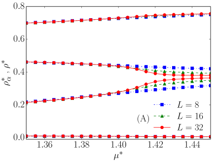
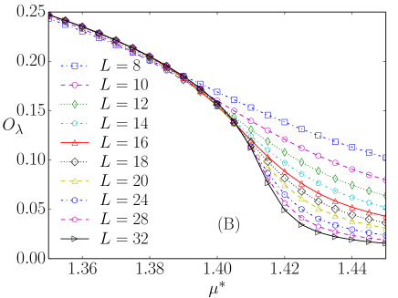
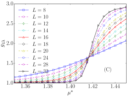
Figure 5: Location of the continuous LDL-HDL transitions for the water model at $T^{*}=0.80$ and different system sizes: $N_{L}=2L^{3}$. At (A) Total reduced density and partial densities, $\rho_{\alpha}$ as functions of $\mu$. (B) (left) Order parameter $O_{\lambda}$ and (left) $g_{4\lambda}$ as a function of $\mu$.

Complementary to the study of the $\theta_{\lambda}$ and $O_{\lambda}$ order parameters described above, the behavior of the specific heat at constant volume for different system sizes were analyzed.

At criticality, it is expected that the specific heat would show a divergence as the thermodynamic limit is approached. The finite-size scaling behavior of the critical exponent of the specific heat, $\alpha$, gives the critical behavior at the infinite system LandauBinderBook . The heat capacity at constant volume ( per lattice site) $c_{V}=\left(\partial{U}/\partial T\right)_{N,V}/V$ is computed from the data obtained from simulations at constant chemical potential through the expression AllenTildesleyBook ,

$$c_{V}=\dfrac{1}{k_{B}T^{2}V}\left[\left\langle\delta{U}^{2}\right\rangle-\dfrac{\left\langle\delta{U}\delta N\right\rangle^{2}}{\left\langle\delta N^{2}\right\rangle}\right]\;.$$ (11)

Here $U$ is the interaction energy of model described in the Table 1, and $N$ is the number of particles. The averages in Eq. (11) are carried out on the grand canonical ensemble.

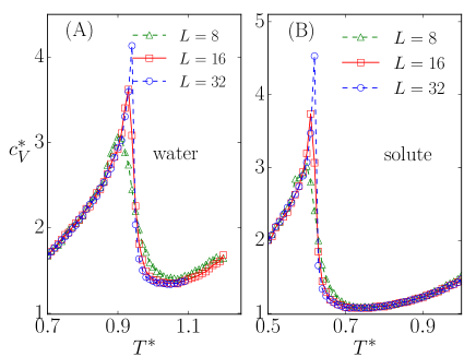
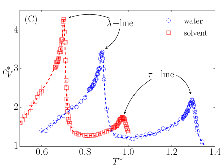
Figure 6: Heat capacity versus reduced temperature for the reduced chemical potentials (A) $\mu^{*}=1.0$ and (B)$\mu^{*}=1.6$ for water and solute respectively for different $L$ values for the $\lambda$-line. The same for $\mu^{*}=1.2$ showing both the $\lambda$ and the $\tau$-lines.

The figure 6 shows the specific heat at constant volume versus temperature at constant $\mu$, illustrating the diverging peak at $T^{*}\simeq 0.9$ for the pure water system and at $T^{*}\simeq 0.6$ for the pure solute, as $L$ increases. The peak in the heat capacity $c_{V}$ in addition to the $O_{\lambda}$ and $\theta_{\lambda}$ behavior is employed to locate the $\lambda-$line.

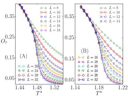
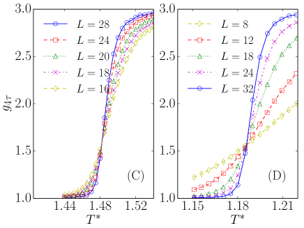
Figure 7: $O_{\tau}$ versus reduced temperature for different systems sizes at chemical potential $\mu=2.0$ for water (A) and solute (B) models. $g_{4\tau}$ versus reduced temperature for different systems sizes at chemical potential $\mu=2.0$ for water (C) and solute (D) models.

The $\tau$-line corresponds to the transition between G and HDL phases. An order parameter based on the symmetry of the ALG model can be defined to quantify the HDL ordering of the configurations. The BCC lattice can be splitted into two interpenetrated cubic sublattices. In the HDL structure, each sublattice adopts a different but complementary orientation. The appropriate order parameter for the $\tau$-line is given by

$$O_{\tau}=\frac{1}{N_{L}}\left|\sum_{i=1}^{N_{L}}l(i)s(i)\right|,$$ (12)

where $l(i)$ depends on the cubic sublattice where the site $i$ stands (with values $-1$, and $+1$ for the two sublattices), and $s(i)$ represents the orientation of the particle at site $i$, with $s(i)=0$ for empty sites. This order parameter is analogous to that for antiferromagnetic Ising models in bipartite lattices. In the figure 7 we show the shape of the order parameter at the HDL-G transition (top panels). For the G phase $O_{\tau}$ vanishes in the thermodynamic limit while for the HDL it remains finite. The approximate location of the transition is obtained by the crossing of the curves for different sizes. Even though the behavior of the order parameter illustrates how the structure of the phases change at the phase transition, it does not provide the precise temperature and chemical potential. The precise location of the transitions can be achieved by looking at the system size dependence of the ratio, $g_{4\tau}$:

$$g_{4\tau}=\frac{\left\langle O_{\tau}^{4}\right\rangle}{\left\langle O_{\tau}^{2}\right\rangle^{2}},$$ (13)

where the brackets indicate average over grand canonical simulations. At the $\tau$-line transition, it is expected that the values of $g_{4\tau}$ become independent of the system size. The figure 7, examples for water and solute of the behavior of $g_{4\tau}(T,N_{L})$ for fixed $\mu$, at the $G-HDL$ transition ($\lambda-$ line) are presented. The value of $g_{4\tau}$ at the crossing region, together with the form of the order parameter suggest three-dimensional Ising criticality. In addition the location of the $\tau$-line can be confirmed by the divergence of the heat capacity.

IV.2 The excess properties of the water-solute mixtures

Next, we explore the mixture of water and solute. The thermodynamic excess properties of the mixture are defined by comparing the values of a given extensive property per mol (or per molecule) with the values of this quantity for an ideal mixture. In the case of the excess volume we have:

$${\bar{V}}^{E}(x,p,T)={\bar{V}}(x,p,T)-\left[(1-x){\bar{V}}_{1}^{0}(p,T)+x{\bar{V}}_{2}^{0}(p,T)\right];$$ (14)

where ${\bar{V}}(x,p,T)$ is the volume per molecule of the mixture at molecular fraction $x$ of the solute (component 2) $x$ (i.e. $x\equiv x_{2}$), ${\bar{V}}_{1}^{0}(p,T)$ and ${\bar{V}}_{2}^{0}(p,T)$ are the volumes per molecule of the pure solvent (component $1$) and pure solute respectively.

The thermodynamic properties for different compositions at constant $T$ and $p$ were computed using GCE simulations coupled to the integration schemes explained in Appendices B and C. In practice, for one component systems we apply an integration scheme to find the line, $\mu(T|p)$ in the plane $\mu-T$ that corresponds to a fixed value, $p$ of the pressure, and for the mixtures we calculate the line $\mu_{1}(\mu_{2}|T,p)$ in the plane $\mu_{1}-\mu_{2}$ that keep fixed the values of $T$ and $p$.

The volumes per molecule was estimated from the simulations as: ${\bar{V}}=V/\langle N\rangle$. The enthalpy, $H$ of a given system is given by: $H=U+pV$, where $U$ is the internal energy (given for the patch-patch interactions). The enthalpy per molecule can be estimated as: $\bar{H}=\left[\langle U\rangle+pV\right]\langle N\rangle$. Whereas the mole fraction for given values of the activities $z_{i}=\exp\left[-\mu_{i}/(k_{B}T)\right]$, is computed as: $\langle x\rangle\simeq\langle N_{2}\rangle/\langle N\rangle$.

The integration procedure provides the results for the different properties at equally spaced discrete values of the activity, $z$, of one of the components, (say component 1) which span from $z_{1}=z_{1}^{(0)}$ (pure solvent) to $z_{1}=0$ (pure solute). For each of these cases the properties of interest, $x(z_{1})$, ${\bar{V}}(z_{1})$, ${\bar{H}}(z_{1}),\cdots$ are computed. Then, to estimate the dependence of the molar properties with the composition these properties are fitted to polynomials of $x$ as:

$$\bar{Y}_{f}(x,T,p)=\sum_{j=0}^{j_{max}}a_{j}^{(Y)}(T,p)x^{j}.$$ (15)

The degree of the polynomial, $j_{max}$, is chosen according to statistical criteria, ensuring that the fitted function provides a good description of the values of the property in the whole range $x\in[0,1]$. Using the functions given in Eq. (15) the excess properties for the volume or the enthalpy are computed as a function of $x$ as:

$$\bar{Y}^{E}(x,T,p)=\bar{Y}_{f}(x,T,p)-x\bar{Y}_{f}(1,T,p)-(1-x)\bar{Y}_{f}(0,T,p).$$ (16)

IV.2.1 The $\lambda_{W}=\lambda_{S}=0.25$ case

First, we analyze the case in which the $B$-$C$ solvent-solute and solute-solute interactions are both attractive and they have the same value namely $\lambda_{W}=\lambda_{S}=0.25$. This represents a system in which in addition the solvent interacts with the solute in two different ways, $B$-$A$ and $B$-$C$, both attractive. In principle this would be the case of the water - alcohol mixture where water forms hydrogen bonds with the alcohol and shows and effective attraction with the alkyl group.

The figure 8 illustrates the excess volume for the pressure and temperature $p^{*}=0.10$ and $T^{*}\simeq 0.3$. As the fraction of the solute increases, the excess volume decreases until it reaches a minimum. The presence of this minimum in a water-solute system is observed in the water-methanol  Abello1973a ; Benson1963a ; Benson1980 ; Panov1976a ; Pattel1985 , in the water-ethanol Ott1993 , in the water-alkanolamines Hepler1994 ; Stec2014 and in the water-hydrophilic ionic liquids Miaja2009 solutions.

The figure 8 also shows the excess enthalpy for our model as a function of the fraction of the solute. The minimum observed in $H^{E}$ is also present in the in water-methanol Tomasziewicz1986 , water-ethanol Ott1986 , water-alkanolamines-Mundhwa2007 and in water with hydrophilic ionic liquids Miaja2009 solutions.

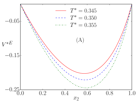
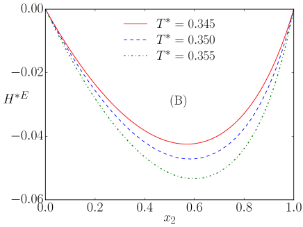
Figure 8: (A) excess volume and (B) excess enthalpy per particle as a function of solute concentration for $\lambda_{S}=0.25$,$\lambda_{W}=0.25$, $p^{*}=0.10$ and several temperatures.

The figure 9 illustrates snapshots of the system as the concentration of the solute is increased. Since the system is in the LDL phase of the solvent, there is one sublattice empty while the other is filled. In the case in which the solute is a hard sphere, as the solute is added to the system it enters in the empty sublattice not competing with the solvent occupation Szortyka2012 . Here this is not the case. The solute enters in the same sublattice occupied by the solvent.

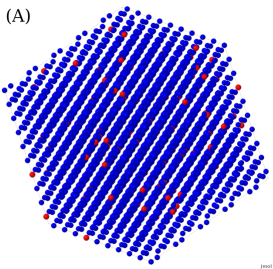
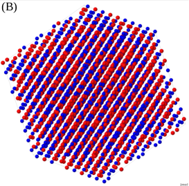
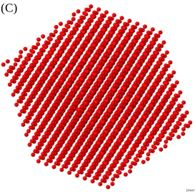
Figure 9: The snapshot of system for $\lambda_{W}=0.25$ and $T^{*}=0.350$. The blue and red spheres represent the water and solute respectively. At (A)-$x_{2}=0.024105$, (B)-$x_{2}=0.704341$ and (C)-$x_{2}=1.$

The behavior of excess volume for this case is similar to that found in quasi-ideal Fuji2012 mixtures of equal size Lennard-Jones particles and different potential well depth. In this quasi-ideal mixture the Lennard-Jones energy parameters are given by, $\epsilon_{22}/\epsilon_{11}=1.50$, $\epsilon_{12}=\left(\epsilon_{11}+\epsilon_{22}\right)/2$, therefore $\epsilon_{12}/\epsilon_{11}=1.25$. At temperature below the critical points and low pressure this mixture have negative excess volume and its behavior as a function of the temperature is qualitatively equal to that of our system. In relation to the excess enthalpy, the same agreement occurs between the quasi-ideal Fuji2012 system and our model with $\lambda_{W}=\lambda_{S}$. The excess enthalpy is negative for entire the range of the mole fraction and the departure from the ideal mixture behavior increases on heating.

In the same mixture if we consider the Lorentz-Berthelot rule $\epsilon_{12}/\epsilon_{11}=\sqrt{\epsilon_{22}/\epsilon_{11}}\simeq 1.225$ (less favorable cross interaction) the excess volume remains negative, but the excess enthalpy becomes positive at temperatures slightly below the critical temperature of component one.

Figure 10: (A) Total density and partial densities and average number of (B) $A$-$B$ bonds between solvent-solvent, solute-solute and solvent-solute and (C) $C$-$B$ bonds between solvent-solvent and solvent-solute for $\lambda_{M}=\lambda_{W}=0.25$, $p^{*}=0.10$ and $T=0.355$.at $T^{*}=0.355$ and $p^{*}=0.10$.

IV.2.2 The $\lambda_{W}=0$ and $\lambda_{S}=0.25$ case

Next, we analyze the case in which the $B$-$C$ solute-solute patch is attractive but the $B$-$C$ solvent-solute patch has no interaction. In this case $\lambda_{W}=0$ while the solute-solute $B$-$C$ is attractive namely $\lambda_{S}=0.25$. This represents a system in which in addition the solvent interacts with the solute only through the $B$-$A$ patch. In principle, this would be the case of the water-alcohol mixture in which the alkyl group is larger than the preceding case and therefore the molecule is less hydrophilic.

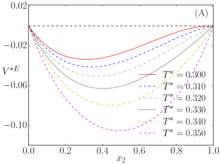
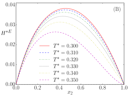
Figure 11: (A) Excess volume and (B) Excess enthalpy $versus$ fraction of solute for various temperatures, $\lambda_{W}=0$, $\lambda_{M}=0.25$ and $p^{*}=0.10$.

The figure 11 illustrates the excess volume and the excess enthalpy as a function of the fraction of the solute for various temperatures. As the fraction of the solute increases, the excess volume decreases until it reaches a minimum while the excess enthalpy has a maximum. This behavior is consistent with the excess volume and enthalpy of mixtures of water and large alcohol molecules such as propanol, butanol and pentanol Ben-Naim2008 ; Marongiu1984 .

The variation of excess properties of this case with respect to the previous one can be explained in terms of the fact that now cross interactions are less attractive, which produces an increase in the excess volume and enthalpy Fuji2012 .

IV.2.3 The $\lambda_{W}=-0.25$ and $\lambda_{S}=0.25$ case

Finally, we analyze the case in which the $B$-$C$ solute-solute patch is attractive but the $B$-$C$ solvent-solute patch is repulsive. In this case $\lambda_{W}=-0.25$ is repulsive while the solute-solute $B$-$C$ is attractive namely $\lambda_{M}=0.25$. This represents a system in which in addition the solvent interacts with the solute through the $B$-$A$ with attraction probably forming hydrogen bonds while show repulsion through the $B$-$C$ patch. In principle this would be the case of the water mixing with molecules that exhibit a hydrophilic region, and eventually, can form a hydrogen bond, but the overall water-solute interaction is repulsive.

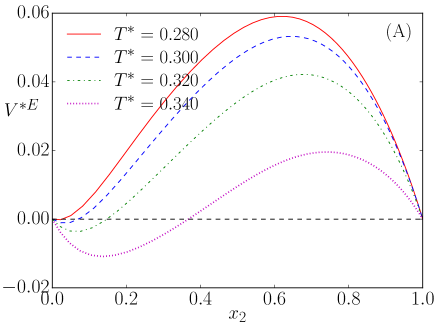
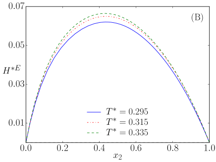
Figure 12: (A) Excess volume and (B) excess enthalpy $versus$ fraction of methanol for various temperatures. $\lambda_{W}=-0.25$, $\lambda_{M}=0.25$ and $p^{*}=0.10$.

The figure 12 illustrates the excess volume and the excess enthalpy as a function of the fraction of the solute for various temperatures. As the fraction of the solute increases, both the excess volume and the excess enthalpy increase until they reach a maximum. This behavior is found in hydrophobic ionic liquids Miaja2009 ; Vatascin2015 .

In this case, the cross interactions are more unfavorable and the excess enthalpy and volume are both positives.

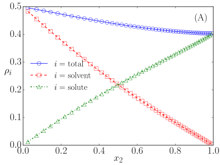
Figure 13: (A) Total density and partial densities and average number of (B) $A$-$B$ bonds between solvent-solvent, solute-solute and solvent-solute and (C) $C$-$B$ bonds between solvent-solvent and solvent-solute for $\lambda_{W}=-0.25$, $T^{*}=0.315$ and $p^{*}=0.10$.

V Conclusions

In this paper a combination of two Associating Lattice Models is employed to represent a mixture of solute and solvent. In the principle the solvent is modeled as a water-like system that exhibits the density and diffusion anomalous behavior present in water. The solute is modeled by molecules that form two types of bonds with water: one attractive hydrogen bond-like, the $A$-$B$ interaction, plus an additional, tunable, $B-C$ interaction.

The pure components, by construction, present very similar phase diagrams. Both present, first (G-LDL/LDL-HDL) and second order ($\lambda-$line/$\tau-$line) transitions, as well as some multicritical points. The phases in coexistence are also the same. The substantial difference happens in the coverage area of phases and the position of multicritical points, and critical lines. The continuous transitions belong to the 3D Ising model universality class.

For the mixture, by tuning the $B$-$C$ patch from attractive to repulsive we were able to qualitatively reproduce the behavior of the excess volume and enthalpy of different types of mixtures.

The mapping of the relative hydrophobicity of the solutes through the $\lambda_{W}$ parameter of the model, allows us to explain the trends of the excess properties of the mixtures as function of the intermolecular effective interaction.

Our result even though based on a very simple model reproduce a mechanism that seems to be present in a large variety aqueous solutions.

Appendix A Computation of the residual entropy

We consider a model defined over the diamond lattice with full occupancy. Each particle (site) carries four arms which point to the four NN sites. In order to compute the residual entropy of the lattice model for water we consider two arms of type $A$ (or +1) and two arms of type $B$ (or -1). A given particle on the lattice can present $q_{W}=4!/(2!2!)=6$ possible configurations. For the lattice model of solute, we consider two arms of type $A$, two of type $B$ and one of type $C$, which leads to $q_{M}=4!/2!=12$ possible orientations of the particle. We set interactions between NN particles, so that the interaction energy is equal to zero for configurations compatible with the ground state of the full model, and greater than zero another case. The pair interactions between NN particles are therefore $u=0$ when are due to the interactions between pair of arms $AB$ or $CB$, and $u=\epsilon>0$ for the other cases ($AA$, $BB$, $AC$, and $CC$).

The partition function of the system can be written as:

$$Q=\sum_{i=1}^{q^{N}}\exp\left[-\frac{U\left(\{{\bf S}\}_{i}\right)}{k_{B}T})\right]$$ (17)

where $N$ being the number of particles (sites) of the system, $U$ the interaction energy and $q$ the number of possible orientations of each particle. $\{{\bf S}\}_{i}$ represent the different configurations of the system. The Helmholtz energy, $A$, is related with the partition function through:

$$\frac{A}{k_{B}T}=-\ln Q$$ (18)

In the limit of infinite temperature, all the possible configurations have the same probability and we get: $A/(k_{B}T)=-N\ln q$. We are interested in the limit at low temperature. Given the fact that we know the partition function at high temperature, we can make use of thermodynamic integrationAllenTildesleyBook ; FrenkelSmitBook to get:

$$A(T)/(k_{B}T)=-N\ln q+\int_{0}^{1/(k_{B}T)}U(T^{\prime})d\left(\frac{1}{k_{B}T^{\prime}}\right);$$ (19)

Taking into account the thermodynamic relation $A=U-TS$, $S$ being the entropy, and defining reduced quantities $U^{*}=U/\epsilon$, and $T^{*}=k_{B}T/\epsilon$, we can get:

$$\frac{S(T)}{k_{B}}=N\ln q_{1}+\frac{U^{*}(T)}{T^{*}}-\int_{0}^{1/T^{*}}U^{*}(T^{\prime}){\textrm{d}}\left(1/T^{\prime*}\right).$$ (20)

In the limit of low temperature the potential energy of the model vanishes, and it is also fulfilled $\lim_{T\rightarrow 0}(U/T)=0$, therefore we get:

$$\frac{S(T)}{k_{B}}\simeq N\ln q-\int_{0}^{1/T^{*}}U^{*}(T^{\prime}){\textrm{d}}\left(1/T^{\prime*}\right);\quad(T^{*}\rightarrow 0)$$ (21)

The residual entropy per particle $s_{0}(N)$ (as a function of the system size) can be computed as:

$$\frac{s_{0}(N)}{k_{B}}=\ln q-\lim_{T^{*}\rightarrow 0}\int_{0}^{1/T^{*}}\frac{U^{*}(N,T^{\prime})}{N}\textrm{d}\left(1/T^{\prime*}\right)$$ (22)

The determination of $s_{0}(N)$ has been carried out using Monte Carlo simulation, in combination with thermodynamic integration, and parallel tempering techniques. Different system sizes were considered in order to carry out a finite-size scaling analysis to determine $s_{0}$ in the thermodynamic limit. Parallel tempering facilitates the equilibration of the systems at low temperature, where the systems reach the ground state (except for some elementary excitations). For the lattice model for water, we have considered different system sizes: $N=8\ell^{3}$, with $\ell=2,3,4,\cdots,14$. In each case we considered 257 values of $(1/T^{*})$; $1/T_{i}^{*}=i\times\Delta(1/T^{*});\quad i=0,1,\cdots,256$; with $\Delta(1/T^{*})=0.050$. The averaged reduced potential energy per particle $u^{*}=U/(N\epsilon)$ is $1$ for $T\rightarrow\infty$, and it almost vanishes for the lowest values of $T$ considered in the integration $u^{*}\ll 10^{-6}$ (for the largest system sizes). It decays rapidly as $T\rightarrow 0$, making possible a reliable cut-off of the integration for a given level of accuracy in the results. In TABLE 2 we present the estimates for $s_{0}(N)$.

Table 2: System-size dependent estimates for the residual entropy presented as $s_{0}^{*}(N)/k_{B}$

$\ell$	2	3	4	5	6
$s_{0}(8\ell^{3})/k_{B}$	0.435774(13)	0.418939(18)	0.414306(18)	0.412543(16)	0.411693(18)
$\ell$	7	8	9	10	11
$s_{0}(8\ell^{3})/k_{B}$	0.411271(19)	0.410988(22)	0.410823(21)	0.410737(24)	0.410645(21)
$\ell$	12	13	14
$s_{0}(8\ell^{3})/k_{B}$	0.410619(14)	0.410574(13)	0.410549(8)

In order to estimate the value of $s_{0}$ in the thermodynamic limit we have considered the scaling relations used by Berg et al. Berg2007 ,

$$s_{0}(N)/k_{B}=s_{0}/k_{B}+a_{1}N^{-\theta};$$ (23)

The fitting of the simulation results given in TABLE 2 to Eq. (23), with $(s_{0}/k_{B})$, $a_{1}$, and $\theta$ being adjustable parameters leads to:

$$s_{0}^{\textrm{(W)}}/k_{B}=0.410\;41\pm 0.000\;02;\;\;\;\theta=0.899\pm 0.005,$$ (24)

where the label $(W)$ refers to water. Considering the quantities $\Omega(N_{L})=\exp[s_{0}(N_{L})/k_{B}]$, and fitting the results to

$$\Omega(N)=\Omega+a_{\Omega}N^{-\theta},$$ (25)

we get

$$\Omega=1.507\;44\pm 0.000\;04;\;\;\;\theta=0.905\pm 0.005.$$ (26)

The values of the exponent $\theta$ agree within statistical uncertainty with the results of Berg et al. Berg2007 . For the residual entropy of the ordinary ice. Interestingly, our estimate of $\Omega$ for our model defined over a system with cubic symmetry and the estimate of for the ordinary ice of Berg et al. Berg2007 : $\Omega^{\rm Ice}=1.507\;38\pm 0.000\;16$; $\theta=0.923(23)$, seem to coincide (at least within error bars) in spite of the different structures of the underlying lattices.

In principle, we could apply the same simulation techniques used for the water in the determination of the residual entropy of the lattice gas model of the solute. However, the value of $s_{0}$ for methanol can be deduced directly from the water results. Given a ground state, the configuration of the water for a system with $N$ molecules (occupied positions) one can build up $2^{N}$ directly related ground states for the methanol model, since the two (undistinguishable) $A$ patches of each particle in the water model correspond to two distinguishable ($A$ and $C$) patches in the methanol model. Therefore, we get:

$$s_{0}^{\textrm{(S)}}=s_{0}^{\textrm{(W)}}+k_{B}\ln 2.$$ (27)

Appendix B Computation of isobars for pure components

The excess properties of binary mixtures are usually measured experimentally at fixed conditions of temperature and pressure Marongiu1984 ; Pattel1985 . For lattice gas models it is neither straightforward not practical the use of simulation in the NPT ensemble. The usual alternative is to carry out simulations in the grand canonical ensemble and compute the pressure by means of thermodynamic integration. Since we are interested in analyzing the excess properties at fixed pressure, we have developed a procedure to build up the lines $\mu(T|p)$ for pure components, i.e. we fix the pressure and compute the chemical potential as a function of temperature at fixed pressure. The objective is to apply this to the ordered phases: LDL and HDL. The pressure at (very) low temperature for these phases can be computed from the ground state analysis. In the GCE the change of the pressure for transformations at constant $T$ and $V$, is given by $dp=\rho d\mu$. The density of the condensed phases at very low temperature hardly changes with $\mu$, therefore, we can integrate the pressure to get.

$$p=p_{0}+\left(\mu-\mu_{0}\right)\rho_{0}$$ (28)

where the values of $p_{0}$, $\mu_{0}$, and $\rho_{0}$ can be taken as those corresponding to the phase coexistence at low temperature (Eqs. 2-5). Once we now how to compute the chemical potential for a given pressure $p$ at a (low) temperature $T_{1}$, we will develop the integration scheme to move on the $(\mu,T)$ plane at the fixed pressure $p$. Imposing $dp=0$ in the differential form for the thermodynamic potential of the GCE we get:

$$d\mu=-\frac{U+pV-N\mu}{NT}dT=-\frac{\tilde{u}-p+\mu\rho}{\rho T}dT$$ (29)

We typically considered systems with $N_{L}=2\times 16^{3}$.

Appendix C The properties of mixtures at fixed $T$ and $p$

The excess properties of mixing are usually defined as the differences between the values of the property of the mixture at a given composition, $x$, and the value of the same property for an ideal mixture of the components at the same conditions of $x$, $T$, and $p$. It is, therefore, desirable to develop simulation strategies to sample in an efficient way different compositions of a given mixture for fixed conditions of temperature and pressure. In order to achieve this aim for our lattice model we have borrowed ideas to form the Gibbs-Duhem integration procedures, as we did for computing isobars of pure components.

The differential form for the grand canonical potential of a binary mixture can be written as:

$$-d\left(\frac{pV}{T}\right)=Ud\left(\frac{1}{T}\right)-\frac{p}{T}dV-\sum_{i=1}^{2}N_{i}d\left(\frac{\mu_{i}}{T}\right);$$ (30)

where $N_{i}$ is the number of molecules of component $i$, and $\mu_{i}$ is the chemical potential of component $i$. If we fix $T$, $p$, and $V$, the chemical potential of the two components can not vary independently when modifying the composition. It should be fulfilled:

$$N_{1}d\mu_{1}+N_{2}d\mu_{2}=0\;.$$ (31)

Using activities $z_{i}\equiv\exp[\mu_{i}/(k_{B}T)]$ to carry out the integration of Eq. (31) we get:

$$\frac{N_{1}}{z_{1}}dz_{1}+\frac{N_{2}}{z_{2}}dz_{2}=0\;.$$ (32)

Let us assume that for some values of $T$, and $p$, we know the values of the activities of the pure components $z_{1}^{(0)}$, and $z_{2}^{(0)}$. We can integrate numerically (using simulation results) the differential equation:

$$dz_{2}=-\frac{N_{1}z_{2}}{N_{2}z_{1}}dz_{1}\;.$$ (33)

For instance, using as starting point $(z_{1}=z_{1}^{(0)},z_{2}=0)$ and considering $z_{1}$ as the independent variable and integrating Eq. (33) up to $z_{1}=0$, we should reach $z_{2}(z_{1}=0)=z_{2}^{(0)}$. This condition provides a powerful consistency check of the thermodynamic integration schemes at constant pressure. The numerical integration of (33) can be carried out using the same numerical procedures as in Sec. B. There is still, a minor technical problem, that appears in the limits $z_{i}\rightarrow 0$; where $N_{i}\rightarrow 0$, and therefore the ratio $(N_{i}/z_{i})$ can not be directly computed from the simulation. This problem can be solved by applying the Widom-insertion test techniqueFrenkelSmitBook to compute the activity of the minority component (which actually has mole fraction $x=0$) as a function of its density. The result can be written as:

$$\lim_{z_{i}\rightarrow 0^{+}}\frac{\rho_{i}^{*}}{z_{i}}=q_{i}\left\langle\exp\left[-\Delta u_{i}/(k_{B}T)\right]\right\rangle;$$ (34)

where $\left\langle\exp\left[-\Delta u_{i}/(k_{B}T)\right]\right\rangle$ represents the average of the Boltzmann exponential over attempts of insertion of a test particle of type $i$ with random position and random orientation on a pure component system of the other component and $q_{i}$ is the number of possible orientations for molecules of type $i$. Results were obtained from simulations of systems with $N_{L}=2\times 16^{3}$.

- (1) H. S. Frank and M. W. Evans, Marjorie, J. Chem. Phys. 13, 507 (1945).
- (2) N. C. Patel, S. I. Sandler, J. Chem. Eng. Data 30, 218 (1985).
- (3) A. Ben-Naim,W. A. M. Navarro and J. M. Leal, Phys. Chem. Chem. Phys. 10, 2451 (2008).
- (4) F. Sha, T. Zhao, B. Guo, F. Zhang, X. Xie and J. Zhang, Phys. Chem. of Liq. 54 , 165(2016).
- (5) J. B. Ott, J. T. Sipowska, M. S. Gruszkiewicx and A. T. Woolley, J. Chem. Thermodynamics 25 , 307(1993).
- (6) B. Marongiu, I. Ferino, R. Monaci, V. Solinas and S. Torrazza, J. Mol. Liq. 28, 229 (1984).
- (7) Y. Maham, T. T. Teng, L. G. Hepler, and A. E. Mather, J. of Sol. Chem. 23 , 195 (1994).
- (8) M. Stec, A. Tatarczuk, D. Spiewak and A. Wilk, J. of Sol. Chem. 43 , 959 (2014).
- (9) C. G. Hanke and R. M. Lynden-Bell J. Phys. Chem. B 107, 10873(2003).
- (10) S. L. Randizio and I. Tomaszkiewicz, Thermochimica Acta 103, 275 (1986).
- (11) I. Tomasziewicz, S. L. Randizio and P. Gierycz, Thermochimica Acta 103, 281(1986).
- (12) J. B. Ott, G. V. Cornett, C. E. Stouffer, B. F. Woodfield,C. Guanquan and J. J. Christensen, J. Chem. Thermodynamics 18, 867(1986).
- (13) M. Mundhwa and A. Henni, J. Chem. Thermodynamics 39, 1439 (2007).
- (14) G. Garcia-Miaja, J. Troncoso and L. Romani, J. Chem. Thermodynamics 41, 161 (2009).
- (15) E. Vatascin and V. Dohnal, J. Chem. Thermodynamics 89, 169 (2015).
- (16) G. C. Benson, P. J. D’arcy, and O. Kiyohara, J. Solution Chem. 9, 931 (1980).
- (17) G. C. Benson, P. J. D’arcy, J. Chem. Eng. Data 27, 439 (1982).
- (18) J. A. V. Butler, D. W. Thomson, and W. H. Maclennan, J. Chem. Soc. 674 (1933).
- (19) D. A. McQuarrie Statistical Mechanics, 1st ed. (Harper & Row New York, 1975)
- (20) R. F. Lama, B. C.-Y Lu, J. Chem. Eng. Data 3, 216 (1965).
- (21) S. Dixit, J. Crain, W. C. K. Poon, J. L. Finney and A. K. Soper, Nature 416, 829 (2002).
- (22) J. H. Guo, Y. Luo, A. Augustsson, S. Kashtanov, J.-E. Rubensson, D. K. Shuh, H. Ågren, and J. Nordgren, Phys. Rev. Lett. 91, 157401 (2003).
- (23) H. J. C. Berendsen, J. R. Grigera and T. P. Straatsma, J. Chem. Phys. 91, 6269 (1987).
- (24) T. Head-Gordon, F. H. Stillinger, J. Chem. Phys. 98, 3313 (1993).
- (25) M. W. Mahoney and W. L. Jorgensen, J. Chem. Phys. 112, 8910 (2000).
- (26) W. L. Jorgensen, D. S. Maxwell, J. Tirado-Rives, J. Am. Chem. Soc. 118, 11225 1996.
- (27) I. Bako, T. Megyes, S. Balint, T. Grosz, and V. Chihaia, Phys. Chem. Chem. Phys. 10 5004 (2008).
- (28) S. K. Allison, J. P. Fox, R. Hargreavesa and S. P. Bates, Phys. Rev. B 71 024201 (2005).
- (29) A. Laaksonen, P. G. Kusalik, and I. M. Svischev, J. Phys. Chem. A 101, 5910 (1997).
- (30) M. Hus, G. Munao and T. Urbic, J. Chem. Phys. 141, 164505 2014.
- (31) Z. Su, S. V. Buldyrev, P. G. Debenedetti, P. J. Rossky and H. E. Stanley, J. Chem. Phys. 136, 044511 (2012).
- (32) M. Girardi and M. Szortyka and M. C. Barbosa, Physica A 386, 692 (2007)
- (33) M. M. Szortyka, M. Girardi, V. B. Henriques, and M. C. Barbosa, J. Chem. Phys. 132, 134904 (2010).
- (34) M. M. Szortyka, M. Girardi, V. B. Henriques, and M. C. Barbosa, J. Chem. Phys. 137, 064905 (2012).
- (35) N. G. Almarza, J. M. Tavares, E. G. Noya and M. M. Telo da Gama, J. Chem. Phys. 137, 244902 (2012).
- (36) M. G. Freire, L. M.N.B.F. Santos, A. M. Fernandes, J. A.P. Coutinho and I. M. Marrucho, Fluid Phase Equilibria 261, 449(2007).
- (37) J. Ranke, A. Othman, P. Fan and A. Muller, Int. J. Mol. Sci. 10, 1271(2009).
- (38) C. Buzano, E. De Stefanis and M. Pretti, J. Chem. Phys. 129, 024506 (2008).
- (39) N. G. Almarza and E. G. Noya, Molec. Phys. 109, 65 (2011).
- (40) M. P. Allen and D. J. Tildesley, Computer Simulation, (Oxford University Press, 1987).
- (41) D. Frenkel and B. Smit, Understanding Molecular Simulation. From Algorithms to Applications, (Academic Press, 1996).
- (42) D. P. Landau and K. Binder, A Guide to Monte Carlo Simulations in Statistical Physics 2nd edition, (Cambridge University Press, 2005).
- (43) R. H. Swendsen, and J.-S. Wang, Phys. Rev. Lett. 57, 2607 (1986).
- (44) D. J. Earl and M. W. Deem, Phys. Chem. Chem. Phys. 7, 3910 (2005).
- (45) D. A. Kofke, Molec. Phys. 7, 1331 (1993).
- (46) D. A. Lavis and G. M. Bell, Statistical Mechanics of Lattice Systems 2 (Springer-Verlag, Berlin 1999).
- (47) M. Yu Panov, Lösungsenthalpie des Wassers in den Alkoholen, 10, 149 (1976).
- (48) L. Abello J. Chim. Phys. Phys,-Chim, Biol. 70, 1355 (1973).
- (49) G. C. Benson J. Phys. Chem. 67, 858 (1963).
- (50) I. Fujihara, Y. Miyano, K. Sakamoto, K. Satoh, K. Nakanishi, Fluid Phase Equilib. 336, 1 (2012).
- (51) B. A. Berg, C. Muguruma and Y. Okamoto, Phys. Rev. B 75, 092202 (2007).