Parallel Evaluation of Multi-Semi-Joins

Abstract

While services such as Amazon AWS make computing power abundantly available, adding more computing nodes can incur high costs in, for instance, pay-as-you-go plans while not always significantly improving the net running time (aka wall-clock time) of queries. In this work, we provide algorithms for parallel evaluation of SGF queries in MapReduce that optimize total time, while retaining low net time. Not only can SGF queries specify all semi-join reducers, but also more expressive queries involving disjunction and negation. Since SGF queries can be seen as Boolean combinations of (potentially nested) semi-joins, we introduce a novel multi-semi-join (MSJ) MapReduce operator that enables the evaluation of a set of semi-joins in one job. We use this operator to obtain parallel query plans for SGF queries that outvalue sequential plans w.r.t. net time and provide additional optimizations aimed at minimizing total time without severely affecting net time. Even though the latter optimizations are NP-hard, we present effective greedy algorithms. Our experiments, conducted using our own implementation Gumbo on top of Hadoop, confirm the usefulness of parallel query plans, and the effectiveness and scalability of our optimizations, all with a significant improvement over Pig and Hive.

1 Introduction

The problem of evaluating joins efficiently in massively parallel systems is an active area of research (e.g., [18, 27, 14, 3, 4, 24, 7, 8, 5, 2]). Here, efficiency can be measured in terms of different criteria, including net time, total time, amount of communication, resource requirements and the number of synchronization steps. As parallel systems aim to bring down the net time, i.e., the difference between query end and start time, it is often considered the most important criterium. The amount of computing power is no longer an issue through the readily availability of services such as Amazon AWS. However, in pay-as-you-go plans, the cost is determined by the total time, that is, the aggregate sum of time spent by all computing nodes. In this paper, we focus on parallel evaluation of queries that minimize total time while retaining low net time. We consider parallel query plans that exhibit low net times and exploit commonalities between queries to bring down the total time.

Semi-joins have played a fundamental role in minimizing communication costs in traditional database systems through their role in semi-join reducers [9, 10], facilitating the reduction of communication in multi-way join computations. In more recent work, Afrati et al. [2] provide an algorithm for computing $n$-ary joins in MapReduce-style systems in which semi-join reducers play a central role. Motivated by the general importance of semi-joins, we study the system aspects of implementing semi-joins in a MapReduce context. In particular, we introduce a multi-semi-join operator MSJ that enables the evaluation of a set of semi-joins in one Mapreduce job while reducing resource usage like total time and requirements on cluster size without sacrificing net time. We then use this operator to efficiently evaluate Strictly Guarded Fragment (SGF) queries [19, 6]. Not only can this query language specify all semi-join reducers, but also more expressive queries involving disjunction and negation.

We illustrate our approach by means of a simple example. Consider the following SGF query $Q$:

$$\begin{array}[]{l}{\tt SELECT}\ (x,y)\ {\tt FROM}\ R(x,y)\\ {\tt WHERE}\ \bigl{(}S(x,y)\ {\tt OR}\ S(y,x)\bigr{)}\ \and\ T(x,z)\end{array}$$

Intuitively, this query asks for all pairs $(x,y)$ in $R$ for which there exists some $z$ such that (1) $(x,y)$ or $(y,x)$ occurs in $S$ and (2) $(x,z)$ occurs in $T$. To evaluate $Q$ it suffices to compute the following semi-joins

$$\begin{array}[]{l}X_{1}\quad\coloneqq\quad R(x,y)\ltimes S(x,y);\\ X_{2}\quad\coloneqq\quad R(x,y)\ltimes S(y,x);\\ X_{3}\quad\coloneqq\quad R(x,y)\ltimes T(x,z);\end{array}$$

store the results in the binary relations $X_{1}$, $X_{2}$, or $X_{3}$, and subsequently compute $\varphi:=(X_{1}\cup X_{2})\cap X_{3}$. Our multi-semi-join operator $\textsf{MSJ}({\cal S})$ (defined in Section 4.2) takes a number of semi-join-equations as input and exploits commonalities between them to optimize evaluation. In our framework, a possible query plan for query $Q$ is of the form:

In this plan, the calculation of $X_{1}$ and $X_{2}$ is combined in a single MapReduce job; $X_{3}$ is calculated in a separate job; and $\textsf{EVAL}(R,\varphi)$ is a third job responsible for computing the subset of $R$ defined by $\varphi$. We provide a cost model to determine the best query plan for SGF queries. We note that, unlike the simple query $Q$ illustrated here, SGF queries can be nested in general. In addition, we also show how to generalize the method to the simultaneous evaluation of multiple SGF queries.

The contributions of this paper can be summarized as follows:

1. We introduce the multi-semi-join operator $\mathop{\ltimes\!\cdot}(\mathcal{S})$ to evaluate a set $\mathcal{S}$ of semi-joins and present a corresponding MapReduce implementation $\textsf{MSJ}(\mathcal{S})$.

2. We present query plans for basic, that is, unnested, SGF queries and propose an improved version of the cost model presented by [35, 26] for estimating their cost. As computing the optimal plan for a given basic SGF query is NP-hard, we provide a fast greedy heuristic Greedy-BSGF.

3. We show that the evaluation of (possibly nested) SGF queries can be reduced to the evaluation of a set of basic SGF queries in an order consistent with the dependencies induced by the former. In this way, computing an optimal plan for a given SGF query (which is NP-hard as well) can be approximated by first determining an optimal subquery ordering, followed by an optimal evaluation of these subqueries. For the former, we present a greedy algorithm called Greedy-SGF.

4. We experimentally assess the effectiveness of Greedy-BSGF and Greedy-SGF and obtain that, backed by an updated cost model, these algorithms successfully manage to bring down total times of parallel evaluation, making it comparable to that of sequential query plans, while still retaining low net times. This is especially true in the presence of commonalities among the atoms of queries. Finally, our system outperforms Pig and Hive in all aspects when it comes to parallel evaluation of SGF queries and displays interesting scaling characteristics.

Outline. This paper is organized as follows. We discuss related work in Section 2. We introduce the strictly guarded fragment (SGF) queries and discuss MapReduce and the accompanying cost model in Section 3. In Section 4, we consider the evaluation of multi-semi-joins and SGF queries. In Section 5, we discuss the experimental validation. We conclude in Section 6.

2 Related work

Recall that first-order logic (FO) queries are equivalent in expressive power to the relational algebra (RA) and form the core fragment of SQL queries (cf., e.g., [1]). Guarded-fragment (GF) queries have been studied extensively by the logicians in 1990s and 2000s, and they emerged from the intensive efforts to obtain a syntactical classification of FO queries with decidable satisfiability problems. For more details, we refer the reader to the highly influential paper by Andreka, van Benthem, and Nemeti [6], as well as survey papers by Grädel and Vardi [22, 34]. In traditional database terms, GF queries are equivalent in expressive power to semi-join algebra [25]. Closely related are freely acyclic GF queries, which are GF queries restricted to using only the $\wedge$ operator and guarded existential quantifiers [30]. Flum et al.[19] introduced the term strictly guarded fragment queries for queries of the form $\exists\bar{y}(\alpha\land\varphi)$. That is, guarded fragment queries without Boolean combinations at the outer level. We consider a slight generalization of these queries as explained in Remark 1.

In general, obtaining the optimal plan in SQL-like query evaluation, even in centralized computation, is a hard problem [13, 23]. Classic works by Yannakakis and Bernstein advocate the use of semi-join operations to optimize the evaluation of conjunctive queries [38, 9, 10]. A lot of work has been invested to optimize query evaluation in Pig [21, 28], Hive [33] and SparkSQL [37] as well as in MapReduce setting in general [12]. None of them target SGF queries directly.

Tao, Lin and Xiao [32] studied minimal MapReduce algorithms, i.e. algorithms that scale linearly to the number of servers in all significant aspects of parallel computation such as reduce compute time, bits of information received and sent, as well as storage space required by each server. They show that, among many other problems, a single semi-join query between two relations can be evaluated by a one round minimal algorithm. This is a simpler problem, as a single basic SGF query may involve multiple semi-join queries. Afrati et al.[2] introduced a generalization of Yannakakis’ algorithm (using semi-joins) to a MapReduce setting. Note that Yannakakis’ algorithm starts with a sequence of semijoin operations, which is a (nested) SGF query in a very restricted form.

3 Preliminaries

We start by introducing the necessary concepts and terminologies. In Section 3.1, we define the strictly guarded fragment queries, while we discuss MapReduce in Section 3.2 and the cost model in Section 3.3.

3.1 Strictly Guarded Fragment Queries

In this section, we define the strictly guarded fragment queries (SGF) [19], but use a non-standard, SQL-like notation for ease of readability.

We assume given a fixed infinite set ${\bf D}=\{a,b,\dots\}$ of data values and a fixed collection of relation symbols ${\bf S}=\{R,S,\dots\}$, disjoint with ${\bf D}$. Every relation symbol $R\in{\bf S}$ is associated with a natural number called the arity of $R$. An expression of the form $R(\bar{a})$ with $R$ a relation symbol of arity $n$ and $\bar{a}\in{\bf D}^{n}$ is called a fact. A database DB is then a finite set of facts. Hence, we write $R(\bar{a})\in\textsf{DB}$ to denote that a tuple $\bar{a}$ belongs to the $R$ relation in DB.

We also assume given a fixed infinite set ${\bf V}=\{x,y,\dots\}$ of variables, disjoint with ${\bf D}$ and ${\bf S}$. A term is either a data value or a variable. An atom is an expression of the form $R(t_{1},\dots,t_{n})$ with $R$ a relation symbol of arity $n$ and each of the $t_{i}$ a term, $i\in[1,n]$. (Note that every fact is also an atom.) A basic strictly guarded fragment (BSGF) query (or just a basic query for short) is an expression of the form

$$Z\coloneqq{\tt SELECT}\ \bar{x}\ {\tt FROM}\ R(\bar{t})\ [\ {\tt WHERE}\ C\ ];$$ (1)

where $\bar{x}$ is a sequence of variables that all occur in the atom $R(\bar{t})$, and the ${\tt WHERE}\ C$ clause is optional. If it occurs, $C$ must be a Boolean combination of atoms. Furthermore, to ensure that queries belong to the guarded fragment, we require that for each pair of distinct atoms $S(\bar{u})$ and $T(\bar{v})$ in $C$ it must hold that all variables in $\bar{u}\cap\bar{v}$ also occur in $\bar{t}$. (See also Remark 1 below.) The atom $R(\bar{t})$ is called the guard of the query, while the atoms occurring in $C$ are called the conditional atoms. We interpret $Z$ as the output relation of the query.

On a database DB, the BSGF query (1) defines a new relation $Z$ containing all tuples $\bar{a}$ for which there is a substitution $\sigma$ for the variables occurring in $\bar{t}$ such that $\sigma(\bar{x})=\bar{a}$, $R(\sigma(\bar{t}))\in\textsf{DB}$, and $C$ evaluates to true in DB under substitution $\sigma$. Here, the evaluation of $C$ in DB under $\sigma$ is defined by recursion on the structure of $C$. If $C$ is $C_{1}\text{{ OR }}C_{2}$, $C_{1}\text{{ AND }}C_{2}$, or $\text{{NOT }}C_{1}$, the semantics is the usual boolean interpretation. If $C$ is an atom $T(\bar{v})$ then $C$ evaluates to true if $\sigma(\bar{t})\in R(\bar{t})\ltimes T(\bar{v})$, i.e., if there exists a $T$-atom in DB that equals $R(\sigma(\bar{t}))$ on those positions where $R(\bar{t})$ and $T(\bar{v})$ share variables.

Example 1.

The intersection $Z_{1}\coloneqq R\cap S$ and the difference $Z_{2}\coloneqq R-S$ between two relations $R$ and $S$ are expressed as follows:

$$Z_{1} \coloneqq {\tt SELECT}\ \bar{x}\ {\tt FROM}\ R(\bar{x})\ {\tt WHERE}\ S(\bar{x});$$

$$Z_{2} \coloneqq {\tt SELECT}\ \bar{x}\ {\tt FROM}\ R(\bar{x})\ {\tt WHERE}\ {\tt NOT}\ S(\bar{x});$$

The semijoin $Z_{3}=R(\bar{x},\bar{y})\ltimes S(\bar{y},\bar{z})$ and the antijoin $Z_{4}=R(\bar{x},\bar{y})\rhd S(\bar{y},\bar{z})$ are expressed as follows:

$$Z_{3} \coloneqq {\tt SELECT}\ \bar{x},\bar{y}\ {\tt FROM}\ R(\bar{x},\bar{y})\ {\tt WHERE}\ S(\bar{y},\bar{z});$$

$$Z_{4} \coloneqq {\tt SELECT}\ \bar{x},\bar{y}\ {\tt FROM}\ R(\bar{x},\bar{y})\ {\tt WHERE}\ {\tt NOT}\ S(\bar{y},\bar{z});$$

The following BSGF query selects all the pairs $(x,y)$ for which $(x,y,4)$ occurs in $R$ and either $(1,x)$ or $(y,10)$ is in $S$, but not both:

$$Z_{5} \coloneqq {\tt SELECT}\ (x,y)\ {\tt FROM}\ R(x,y,4)$$

$${\tt WHERE}\ (S(1,x)\ \and\ {\tt NOT}\ S(y,10))$$

$${\tt OR}\ ({\tt NOT}\ S(1,x)\ \and\ S(y,10));$$

Finally, the traditional star semi-join between $R(x_{1},\dots,x_{n})$ and relations $S_{i}(x_{i},y_{i})$, for $i\in[1,n]$, is expressed as follows:

$$Z_{6} \coloneqq {\tt SELECT}\ (x_{1},\dots,x_{n})\ {\tt FROM}\ R(x_{1},\ldots,x_{n})$$

$${\tt WHERE}\ S(x_{1},y_{1})\ \and\dots\ \and\ S(x_{n},y_{n});\qquad\hfill\Box$$

A strictly guarded fragment (SGF) query is a collection of BSGFs of the form $Z_{1}\coloneqq\xi_{1};\ldots;Z_{n}\coloneqq\xi_{n};$ where each $\xi_{i}$ is a BSGF that can mention any of the predicates $Z_{j}$ with $j<i$. On a database DB, the SGF query then defines a new relation $Z_{n}$ where every occurrence of $Z_{i}$ is defined by evaluating $\xi_{i}$.

Example 2.

Let Amaz, BN, and BD be relations containing tuples (title, author, rating) corresponding to the books found at Amazon, Barnes and Noble, and Book Depository, respectively. Let Upcoming contain tuples (newtitle, author) of upcoming books. The following query selects all the upcoming books (newtitle, author) of authors that have not yet received a “bad” rating for the same title at all three book retailers; $Z_{2}$ is the output relation:

$$Z_{1} \coloneqq {\tt SELECT}\ \textrm{aut}\ {\tt FROM}\ \textbf{Amaz}(\textrm{ttl},\textrm{aut},\textsf{"bad"})$$

$${\tt WHERE}\ \textbf{BN}(\textrm{ttl},\textrm{aut},\textsf{"bad"})\ \and\ \textbf{BD}(\textrm{ttl},\textrm{aut},\textsf{"bad"});$$

$$Z_{2} \coloneqq {\tt SELECT}\ (\textrm{new},\textrm{aut})\ {\tt FROM}\ \textbf{Upcoming}(\textrm{new},\textrm{aut})$$

$${\tt WHERE}\ {\tt NOT}\ Z_{1}(\textrm{aut});$$

Note that this query cannot be written as a basic SGF query, since the atoms in the query computing $Z_{1}$ must share the ttl variable, which is not present in the guard of the query computing $Z_{2}$. $\Box$

Remark 1.

The syntax we use here differs from the traditional syntax of the Guarded Fragment [19], and is actually closer in spirit to join trees for acyclic conjunctive queries [9, 11], although we do allow disjunction and negation in the where clause. In the traditional syntax, a projection in the guarded fragment is only allowed in the form $\exists\bar{w}R(\bar{x})\wedge\varphi(\bar{z})$ where all variables in $\bar{z}$ must occur in $\bar{x}$. One can obtain a query in the traditional syntax of the guarded fragment from our syntax by adding extra projections for the atoms in $C$. For example,

$${\tt SELECT}\ x\ {\tt FROM}\ R(x,y)\ {\tt WHERE}\ S(x,z_{1})\ \and\ {\tt NOT}\ S(y,z_{2})$$

becomes $\exists y(R(x,y)\wedge(\exists z_{1})S(x,z_{1})\wedge\neg(\exists z_{2})S(y,z_{2}))$. We note that this transformation increases the nesting depth of the query. $\Box$

3.2 MapReduce

We briefly recall the Map/Reduce model of computation (MR for short), and its execution in the open-source Hadoop framework [17, 36]. An MR job is a pair $(\mu,\rho)$ of functions, where $\mu$ is called the map and $\rho$ the reduce function. The execution of an MR job on an input dataset $I$ proceeds in two stages. In the first stage, called the map stage, each fact $f\in I$ is processed by $\mu$, generating a collection $\mu(f)$ of key-value pairs of the form $\left\langle k:v\right\rangle$. The total collection $\bigcup_{f\in I}\mu(f)$ of key-value pairs generated during the map phase is then grouped on the key, resulting in a number of groups, say $\left\langle k_{1}:V_{1}\right\rangle,\dots,\left\langle k_{n}:V_{n}\right\rangle$ where each $V_{i}$ is a set of values. Each group $\left\langle k_{i}:V_{i}\right\rangle$ is then processed by the reduce function $\rho$ resulting again in a collection of key-value pairs per group. The total collection $\bigcup_{i}\rho(\left\langle k_{i}:V_{i}\right\rangle)$ is the output of the MR job.

An MR program is a directed acyclic graph of MR jobs, where an edge from job $(\mu,\rho)\to(\mu^{\prime},\rho^{\prime})$ indicates that $(\mu^{\prime},\rho^{\prime})$ operates on the output of $(\mu,\rho)$. We refer to the length of the longest path in an MR program as the number of rounds of the program.

3.3 Cost Model for MapReduce

$$\hbox to0.0pt{$\,\underbrace{\phantom{\text{reap}\rightarrow\text{m}}}_{\textsc{\scriptsize Input}}\underbrace{\phantom{\text{ap}\rightarrow\text{sort}\rightarrow\text{merge}\rightarrow\text{trans.}\rightarrow\text{merge}\rightarrow\text{red}}}_{\textsc{\scriptsize Intermediate Data}}\underbrace{\phantom{\text{uce}\rightarrow\text{priti}}}_{\textsc{\scriptsize Output}}$\hss}\overbrace{\text{read}\rightarrow\text{map}\rightarrow\text{sort}\rightarrow\text{merge}}^{\textsc{\scriptsize Map Phase}}\rightarrow\overbrace{\text{trans.}\rightarrow\text{merge}\rightarrow\text{reduce}\rightarrow\text{write}}^{\textsc{\scriptsize Reduce Phase}}$$

Figure 1: A depiction of the inner workings of Hadoop MR.

As our aim is to reduce the total cost of parallel query plans, we need a cost model that estimates this metric for a given MR job. We briefly touch upon a cost model for analyzing the I/O complexity of an MR job based on the one introduced in [35, 26] but with a distinctive difference. The adaptation we introduce, and that is elaborated upon below, takes into account that the map function may have a different input/output ratio for different parts of the input data.

While conceptually an MR job consists of only the map and reduce stage, its inner workings are more intricate. Figure 1 summarizes the steps in the execution of an MR job. See [36, Figure 7-4, Chapter 7] for more details. The map phase involves (i) applying the map function on the input; (ii) sorting and merging the local key-value pairs produced by the map function, and (iii) writing the result to local disk.

Let $\mathcal{I}_{1}\cup\cdots\cup\mathcal{I}_{k}$ denote the partition of the input tuples such that the mapper behaves uniformly on every data item in $\mathcal{I}_{i}$. Let $N_{i}$ be the size (in MB) of $\mathcal{I}_{i}$, and let $M_{i}$ be the size (in MB) of the intermediate data output by the mapper on $\mathcal{I}_{i}$. The cost of the map phase on $\mathcal{I}_{i}$ is:

$$\operatorname{\text{\it cost}}_{\text{\it map}}(N_{i},M_{i}) = h_{r}N_{i}+\operatorname{merge_{\text{\it map}}}(M_{i})+l_{w}M_{i},$$

where $\operatorname{merge_{\text{\it map}}}(M_{i})$, denoting the cost of sort and merge in the map stage, is expressed by

$$\operatorname{merge_{\text{\it map}}}(M_{i}) = (l_{r}+l_{w})M_{i}\log_{D}\bigg{\lceil}\dfrac{\nicefrac{{(M_{i}+\widehat{M}_{i})}}{{m_{i}}}}{\mathit{buf}_{\text{\it map}}}\bigg{\rceil}.$$

See Table 1 for the meaning of the variables $h_{r}$, $l_{w}$, $l_{r}$, $l_{w}$, $D$, $\widehat{M}_{i}$, $m_{i}$, and $\mathit{buf}_{\text{\it map}}$. The total cost incurred in the map phase equals the sum

$$\sum_{i=1}^{k}\ \operatorname{\text{\it cost}}_{\text{\it map}}(N_{i},M_{i}).$$ (2)

Note that the cost model in [35, 26] defines the total cost incurred in the map phase as

$$\operatorname{\text{\it cost}}_{\text{\it map}}\left(\sum_{i=1}^{k}N_{i},\sum_{i=1}^{k}M_{i}\right).$$ (3)

The latter is not always accurate. Indeed, consider for instance an MR job whose input consists of two relations $R$ and $S$ where the map function outputs many key-value pairs for each tuple in $R$ and at most one key-value pair for each tuple in $S$, e.g., because of filtering. This difference in map output may lead to a non-proportional contribution of both input relations to the total cost. Hence, as shown by Equation (2), we opt to consider different inputs separately. This cannot be captured by map cost calculation of Equation (3), as it considers the global average map output size in the calculation of the merge cost. In Section 5, we illustrate this problem by means of an experiment that confirms the effectiveness of the proposed adjustment.

To analyze the cost in the reduce phase, let $M=\sum_{i=1}^{k}M_{i}$. The reduce stage involves (i) transferring the intermediate data (i.e., the output of the map function) to the correct reducer, (ii) merging the key-value pairs locally for each reducer, (iii) applying the reduce function, and (iv) writing the output to hdfs. Its cost will be

$$\operatorname{\text{\it cost}}_{\text{\it red}}(M,K) = tM+\operatorname{merge_{\text{\it red}}}(M)+h_{w}K,$$

where $K$ is the size of the output of the reduce function (in MB). The cost of merging equals

$$\operatorname{merge_{\text{\it red}}}(M) =(l_{r}+l_{w})M\log_{D}\bigg{\lceil}\dfrac{\nicefrac{{M}}{{r}}}{\mathit{buf}_{\text{\it red}}}\bigg{\rceil}.$$

The total cost of an MR job equals the sum

$$\operatorname{\text{\it cost}}_{\text{\it h}}+\sum_{i=1}^{k}\operatorname{\text{\it cost}}_{\text{\it map}}(N_{i},M_{i})+\operatorname{\text{\it cost}}_{\text{\it red}}(M,K),$$

where $\operatorname{\text{\it cost}}_{\text{\it h}}$ is the overhead cost of starting an MR job.

$l_{r}$	local disk read cost (per MB)
$l_{w}$	local disk write cost (per MB)
$h_{r}$	hdfs read cost (per MB)
$h_{w}$	hdfs write cost (per MB)
$t$	transfer cost (per MB)
$\widehat{M}_{i}$	map output meta-data for $\mathcal{I}_{i}$ (in MB)
$m_{i}$	number of mappers for $\mathcal{I}_{i}$
$r$	number of reducers
$D$	external sort merge factor
$\mathit{buf}_{\text{\it map}}$	map task buffer limit (in MB)
$\mathit{buf}_{\text{\it red}}$	reduce task buffer limit (in MB)

Table 1: Description of constants used in the cost model.

4 Evaluating multi-semi-join and SGF Queries

In this section, we describe how SGF queries can be evaluated. We start by introducing some necessary building blocks in Sections 4.1 to 4.3, and describe the evaluation of BSGF queries and multiple BSGF queries in Section 4.4 and 4.5, respectively. These are then generalized to the full fragment of SGF queries in Section 4.6 and 4.7.

First, we introduce some additional notation. We say that a tuple $\bar{a}=(a_{1},\ldots,a_{n})\in{\bf D}^{n}$ of $n$ data values conforms to a vector $\bar{t}=(t_{1},\ldots,t_{n})$ of terms, if

1. $\forall i,j\in[1,n]$, $t_{i}=t_{j}$ implies $a_{i}=a_{j}$; and,

2. $\forall i\in[1,n]$ if $t_{i}\in{\bf D}$, then $t_{i}=a_{i}$.

For instance, $(1,2,1,3)$ conforms to $(x,2,x,y)$. Likewise, a fact $T(\bar{a})$ conforms to an atom $U(\bar{t})$ if $T=U$ and $\bar{a}$ conforms to $\bar{t}$. We write $T(\bar{a})\models U(\bar{t})$ to denote that $T(\bar{a})$ conforms to $U(\bar{t})$. If $f=R(\bar{a})$ is a fact conforming to an atom $\alpha=R(\bar{t})$ and $\bar{x}$ is a sequence of variables that occur in $\bar{t}$, then the projection $\pi_{\alpha;\bar{x}}(f)$ of $f$ onto $\bar{x}$ is the tuple $\bar{b}$ obtained by projecting $\bar{a}$ on the coordinates in $\bar{x}$. For instance, let $f=R(1,2,1,3)$ and $\alpha=R(x,y,x,z)$. Then, $R(1,2,1,3)\models R(x,y,x,z)$ and hence $\pi_{\alpha;x,z}(f)=(1,3)$.

4.1 Evaluating One Semi-Join

As a warm-up, let us explain how single semi-joins can be evaluated in MR. A single semi-join is a query of the form

$$Z:={\tt SELECT}\ \bar{w}\ {\tt FROM}\ \alpha\ {\tt WHERE}\ \kappa;$$ (4)

where both $\alpha$ and $\kappa$ are atoms. For notational convenience, we will denote this query simply by $\pi_{\bar{w}}(\alpha\ltimes\kappa)$.

To evaluate (4), one can use the following one round repartition join [12]. The mapper distinguishes between guard facts (i.e., facts in DB conforming to $\alpha$) and conditional facts (i.e., facts in DB conforming to $\kappa$). Specifically, let $\bar{z}$ be the join key, i.e., those variables occurring in both $\alpha$ and $\kappa$. For each guard fact $f$ such that $f\models\alpha$, the mapper emits the key-value pair $\left\langle\pi_{\alpha;\bar{z}}(f):[\textsc{Req}\,\kappa;\textsc{Out}\,\pi_{\alpha;\bar{w}}(f)]\right\rangle$. Intuitively, this pair is a “message” sent by guard fact $f$ to request whether a conditional fact $g\models\kappa$ with $\pi_{\kappa;\bar{z}}(g)=\pi_{\alpha;\bar{z}}(f)$ exists in the database, stating that if such a conditional fact exists, the tuple $\pi_{\alpha;\bar{w}}(f)$ should be output. Conversely, for each conditional fact $g\models\kappa$, the mapper emits a message of the form $\left\langle\pi_{\kappa;\bar{z}}(g):[\textsc{Assert}\,\kappa]\right\rangle$, asserting the existence of a $\kappa$-conforming fact in the database with join key $\pi_{\kappa;\bar{z}}(g)$. On input $\left\langle\bar{b}:V\right\rangle$, the reducer outputs all tuples $\bar{a}$ to relation $Z$ for which $[\textsc{Req}\,\kappa;\textsc{Out}\,\bar{a}]\in V$, provided that $V$ contains at least one assert message.

Example 3.

Consider the query $Z\coloneqq\pi_{x}(R(x,z)\ltimes S(z,y))$ and let $I$ contain the facts $\{R(1,2),R(4,5),S(2,3)\}$. Then the mapper emits key-value pairs $\left\langle 2:[\textsc{Req}\,S(z,y);\textsc{Out}\,1]\right\rangle$, $\left\langle 5:[\textsc{Req}\,S(z,y);\textsc{Out}\,4]\right\rangle$ and, $\left\langle 2:[\textsc{Assert}\,S(z,y)]\right\rangle$, which after reshuffling result in groups $\left\langle 5:\{[\textsc{Req}\,S(z,y);\textsc{Out}\,4]\}\right\rangle$ and, $\left\langle 2:\{[\textsc{Req}\,S(z,y);\textsc{Out}\,1],[\textsc{Assert}\,S(z,y)]\}\right\rangle$. Only the reducer processing the second group produces an output, namely the fact $Z(1)$.    $\Box$

Cost Analysis

To compare the cost of separate and combined evaluation of multiple semi-joins in the next section, we first illustrate how to analyze the cost of evaluating a single semi-join using the cost model described above. Hereto, let $|\alpha|$ and $|\kappa|$ denote the total size of all facts that conform to $\alpha$ and $\kappa$, respectively. Five values are required for estimating the total cost: $N_{1},N_{2},M_{1},M_{2}$ and $K$. We can now choose $M_{1}=|\alpha|$ and $M_{2}=|\kappa|$. For simplicity, we assume that key-value pairs output by the mapper have the same size as their corresponding input tuples, i.e., $N_{1}=M_{1}$ and $N_{2}=M_{2}$. Finally, the output size $K$ can be approximated by its upper bound $N_{1}$. Correct values for meta-data size and number of mappers can be derived from the number of input records and the system settings.

4.2 Evaluating a Collection of Semi-Joins

Since a BSGF query is essentially a Boolean combination of semi-joins, it can be computed by first evaluating all semi-joins followed by the evaluation of the Boolean combination. In the present section, we introduce a single-job MR program MSJ that evaluates a set of semi-joins in parallel. In the next section we introduce the single-job MR program EVAL to evaluate the Boolean combination.

We introduce a unary multi-semi-join operator $\mathop{\ltimes\!\cdot}({\cal S})$ that takes as input a set of equations ${\cal S}=\{X_{1}\coloneqq\pi_{\bar{x}_{1}}(\alpha_{1}\ltimes\kappa_{1}),\dots,X_{n}\coloneqq\pi_{\bar{x}_{n}}(\alpha_{n}\ltimes\kappa_{n})\}$. It is required that the $X_{i}$ are all pairwise distinct and that they do not occur in any of the right-hand sides. The semantics is straightforward: the operator computes every semi-join $\pi_{\bar{x}_{i}}(\alpha_{i}\ltimes\kappa_{i})$ in ${\cal S}$ and stores the result in the corresponding output relation $X_{i}$.

We now expand the MR job described in Section 4.1 into a job that computes $\mathop{\ltimes\!\cdot}({\cal S})$ by evaluating all semi-joins in parallel. Let $\bar{z}_{i}$ be the join key of semi-join $\pi_{\bar{x}_{i}}(\alpha_{i}\ltimes\kappa_{i})$. Algorithm 1 shows the single MR job $\textsf{MSJ}({\cal S})$ that evaluates all $n$ semi-joins at once. More specifically, MSJ simulates the repartition join of Section 4.1, but outputs request messages for all the guard facts at once (i.e., those facts conforming to one of the $\alpha_{i}$ for $i\in[1,n]$). Similarly, assert messages are generated simultaneously for all of the conditional facts (i.e., those facts conforming to one of the $\kappa_{i}$ for $i\in[1,n]$). The reducer then reconciles the messages concerning the same $\kappa_{i}$. That is, on input $\left\langle\bar{b}:V\right\rangle$, the reducer outputs the tuple $\bar{a}$ to relation $X_{i}$ for which $[\textsc{Req}\,(\kappa,i);\textsc{Out}\,\bar{a}]\in V$, provided that $V$ contains at least one message of the form $[\textsc{Assert}\,\kappa]$. The output therefore consists of the relations $X_{1},\dots,X_{n}$, with each $X_{i}$ containing the result of evaluating $\pi_{\bar{x}_{i}}(\alpha_{i}\ltimes\kappa_{i})$.

Combining the evaluation of a collection of semi-joins into a single MSJ job avoids the overhead of starting multiple jobs, reads every input relation only once, and can reduce the amount of communication by packing similar messages together (cf. Section 5.1). At the same time, grouping all semi-joins together can potentially increase the average load of map and/or reduce tasks, which directly leads to an increased net time. These trade-offs are made more apparent in the following analysis and are taken into account in the algorithm Greedy-BSGF introduced in Section 4.4.

Algorithm 1 MSJ($X_{1}\coloneqq\pi_{\bar{x}_{1}}(\alpha_{1}\ltimes\kappa_{1}),\dots,X_{n}\coloneqq\pi_{\bar{x}_{n}}(\alpha_{n}\ltimes\kappa_{n})$)

1:function Map(Fact $f$)

2:     buff = [ ]

3:     for every $i$ such that $f\models\alpha_{i}$ do

4:         buff += $\left\langle\pi_{\alpha_{i};\bar{z}_{i}}(f):[\textsc{Req}\,(\kappa_{i},i);\textsc{Out}\,\pi_{\alpha_{i};\bar{x}_{i}}(f)]\right\rangle$      

5:     for every $i$ such that $f\models\kappa_{i}$ do

6:         buff += $\left\langle\pi_{\kappa_{i};\bar{z}_{i}}(f):[\textsc{Assert}\,\kappa_{i}]\right\rangle$      

7:     emit buffer

8:

9:function Reduce$(\left\langle k:V\right\rangle)$

10:     for all  $[\textsc{Req}\,\kappa_{i};\textsc{Out}\,\bar{a}]$ in $V$ do

11:         if $V$ contains $[\textsc{Assert}\,\kappa_{i}]$ then

12:              add $\bar{a}$ to $X_{i}$               

Cost Analysis

Let all $\kappa_{i}$’s be different atoms and $\alpha_{1}=\cdots=\alpha_{n}=\alpha$. A similar analysis can be performed for other comparable scenarios. As before, we assume that the size of the key-value pair is the same as the size of the conforming fact, and all tuples conform to their corresponding atom. The cost of $\textsf{MSJ}(\mathcal{S})$, denoted by $\operatorname{\text{\it cost}}(\mathcal{S})$, equals

$$\operatorname{\text{\it cost}}_{\text{\it h}}+\operatorname{\text{\it cost}}_{\text{\it map}}(|\alpha|,n|\alpha|)+\sum_{i=1}^{n}\operatorname{\text{\it cost}}_{\text{\it map}}(|\kappa_{i}|,|\kappa_{i}|)\\ +\operatorname{\text{\it cost}}_{\text{\it red}}\Big{(}n|\alpha|+\sum_{i=1}^{n}|\kappa_{i}|,\sum_{i=1}^{n}|X_{i}|\Big{)},$$ (5)

where $|X_{i}|$ is the size of the output relation $X_{i}$. If we evaluate each $X_{i}$ in a separate MR job, the total cost is:

$$\sum_{i=1}^{n}\left(\!\begin{array}[]{l}\operatorname{\text{\it cost}}_{\text{\it h}}+\operatorname{\text{\it cost}}_{\text{\it map}}(|\alpha|,|\alpha|)+\operatorname{\text{\it cost}}_{\text{\it map}}(|\kappa_{i}|,|\kappa_{i}|)\\ +\operatorname{\text{\it cost}}_{\text{\it red}}(|\alpha|+|\kappa_{i}|,|X_{i}|)\end{array}\!\right)$$ (6)

So, single-job evaluation of all $X_{i}$’s is more efficient than separate evaluation iff Equation (5) is less than Equation (6).

4.3 Evaluating Boolean Combinations

Let $X_{0},X_{1},\dots X_{n}$ be relations with the same arity and let $\varphi$ be a Boolean formula over $X_{1},\dots X_{n}$. It is straightforward to evaluate $X_{0}\land\varphi$ in a single MR job: on each fact $X_{i}(\bar{a})$, the mapper emits $\left\langle\bar{a}:i\right\rangle$. The reducer hence receives pairs $\left\langle\bar{a}:V\right\rangle$ with $V$ containing all the indices $i$ for which $\bar{a}\in X_{i}$, and outputs $\bar{a}$ only if the Boolean formula, obtained from $X_{0}\land\varphi$ by replacing every $X_{i}$ with true if $i\in V$ and false otherwise, evaluates to true. For instance, if $\varphi=X_{1}\land X_{2}\land\neg X_{3}$, it will emit $\bar{a}$ only if $V$ contains 0, $1$ and $2$ but not $3$.

We denote this MR job as $\textsf{EVAL}(X_{0},\varphi)$. We emphasize that multiple Boolean formulas $Y_{1}\land\varphi_{1},\ldots,Y_{n}\land\varphi_{n}$ with distinct sets of variables can be evaluated in one MR job which we denote as $\textsf{EVAL}(Y_{1},\varphi_{1},\ldots,Y_{n},\varphi_{n})$.

Cost Analysis

Let $|X_{i}|$ be the size of relation $X_{i}$. Then, when $|\varphi|$ is the size of the output, $\operatorname{\text{\it cost}}(\textsf{EVAL}(X_{0},\varphi))$ equals

$$\operatorname{\text{\it cost}}_{\text{\it h}}+\sum_{i=0}^{n}\operatorname{\text{\it cost}}_{\text{\it map}}(|X_{i}|,|X_{i}|)+\operatorname{\text{\it cost}}_{\text{\it red}}\big{(}\sum_{i=0}^{n}|X_{i}|,|\varphi|\big{)}.$$ (7)

4.4 Evaluating BSGF Queries

(a)

(b)

(c)

Figure 2: Different possible query plans for the query given in Example 4. Here, $X_{1}\coloneqq R(x,y)\ltimes S(x,z)$, $X_{2}\coloneqq R(x,y)\ltimes T(y)$, $X_{3}\coloneqq R(x,y)\ltimes U(x)$ and $Z\coloneqq X_{1}\land(X_{2}\lor\neg X_{3})$; trivial projections are omitted.

We now have the building blocks to discuss the evaluation of basic queries. Consider the following basic query $Q$:

$$Z\coloneqq{\tt SELECT}\ \bar{w}\ {\tt FROM}\ R(\bar{t})\ {\tt WHERE}\ C.\qquad$$

Here, $C$ is a Boolean combination of conditional atoms $\kappa_{i}$, for $i\in[1,n]$, that can only share variables occurring in $\bar{t}$. Note that it is implicit that $\kappa_{1},\ldots,\kappa_{n}$ are all different atoms. Furthermore, let ${\cal S}$ be the set of equations $\{X_{1}\coloneqq\pi_{\bar{w}}(R(\bar{t})\ltimes\kappa_{1}),\dots,X_{n}\coloneqq\pi_{\bar{w}}(R(\bar{t})\ltimes\kappa_{n})\}$ and let $\varphi_{C}$ be the Boolean formula obtained from $C$ by replacing every conditional atom $\kappa_{i}$ by $X_{i}$.

Then, for every partition $\{\mathcal{S}_{1},\ldots,\mathcal{S}_{p}\}$ of $\mathcal{S}$, the following MR program computes $Q$:

We refer to any such program as a basic MR program for $Q$. Notice that all MSJ jobs can be executed in parallel. So, the above program consists in fact of two rounds, but note that there are $p+1$ MR jobs in total: one for each $\textsf{MSJ}(\mathcal{S}_{i})$, and one for $\textsf{EVAL}(R,\varphi_{C})$.

Example 4.

Figure 2 shows three alternative basic MR programs for the following query:

$$Z \coloneqq {\tt SELECT}\ x,y\ {\tt FROM}\ R(x,y)$$ (8)

$${\tt WHERE}\ S(x,z)\ \and\ (T(y)\ {\tt OR}\ {\tt NOT}\ U(x))$$

In alternative (a), all semijoins $X_{1},X_{2},X_{3}$ are evaluated as separate jobs. In alternative (b), $X_{1}$ and $X_{3}$ are computed in one job, while $X_{2}$ is computed separately. In alternative (c), all semijoins $X_{1},X_{2},X_{3}$ are computed in a single job.  $\Box$

Cost Analysis

When $\mathcal{S}$ is partitioned into $\mathcal{S}_{1}\cup\cdots\cup\mathcal{S}_{p}$, the cost of the MR program is:

$$\operatorname{\text{\it cost}}(\textsf{EVAL}(R,\varphi_{C}))+\sum_{i=1}^{p}\operatorname{\text{\it cost}}(\mathcal{S}_{i}),$$ (9)

where the cost of $\operatorname{\text{\it cost}}(\mathcal{S}_{i})$ is as in Equation (5).

Computing the Optimal Partition

By BSGF-Opt we denote the problem that takes a BSGF query $Q$ as above and computes a partition $\mathcal{S}_{1}\cup\cdots\cup\mathcal{S}_{p}$ of $\mathcal{S}$ such that its total cost as computed in Equation (9) is minimal. The Scan-Shared Optimal Grouping problem, which is known to be NP-hard, is reducible to this problem [26]:

Theorem 1.

The decision variant of BSGF-Opt is NP-complete.

While for small queries the optimal solution can be found using a brute-force search, for larger queries we adopt the fast greedy heuristic introduced by Wang et al[35]. For two disjoint subsets $\mathcal{S}_{i},\mathcal{S}_{j}\subseteq\mathcal{S}$, define:

$$\operatorname{gain}(\mathcal{S}_{i},\mathcal{S}_{j})=\operatorname{\text{\it cost}}(\mathcal{S}_{i})+\operatorname{\text{\it cost}}(\mathcal{S}_{j})-\operatorname{\text{\it cost}}(\mathcal{S}_{i}\cup\mathcal{S}_{j}).$$

That is, $\operatorname{gain}(\mathcal{S}_{i},\mathcal{S}_{j})$ denotes the cost gained by evaluating $\mathcal{S}_{i}\cup\mathcal{S}_{j}$ in one MR job rather than evaluating each of them separately. For a partition $\mathcal{S}_{1}\cup\cdots\cup\mathcal{S}_{p}$, our heuristic algorithm greedily finds a pair $i,j\in[p]\times[p]$ such that $i\neq j$ and $\operatorname{gain}(\mathcal{S}_{i},\mathcal{S}_{j})>0$ is the greatest. If there is such a pair $i,j$, we merge $\mathcal{S}_{i}$ and $\mathcal{S}_{j}$ into one set. We iterate such heuristic starting with the trivial partition $\mathcal{S}_{1}\cup\cdots\cup\mathcal{S}_{n}$, where each $\mathcal{S}_{i}=\{X_{i}\coloneqq\pi_{\bar{w}}(R(\bar{t})\ltimes\kappa_{i})\}$. The algorithm stops when there is no pair $i,j$ for which $\operatorname{gain}(\mathcal{S}_{i},\mathcal{S}_{j})>0$. We refer to this algorithm as Greedy-BSGF. For a BSGF query $Q$, we denote by $\textsf{OPT}(Q)$ the optimal (least cost) basic MR program for $Q$, and by $\textsf{GOPT}(Q)$ we denote the program computed by Greedy-BSGF.

4.5 Evaluating Multiple BSGF Queries

The approach presented in the previous section can be readily adapted to evaluate multiple BSGF queries. Indeed, consider a set of $n$ BSGF queries, each of the form

$$Z_{i}\coloneqq{\tt SELECT}\ \bar{w}_{i}\ {\tt FROM}\ R_{i}(\bar{t}_{i})\ {\tt WHERE}\ C_{i}$$

where none of the $C_{i}$ can refer to any of the $Z_{j}$. A corresponding MR program is then of the form

The child nodes constitute a partition of all the necessary semi-joins. Again, $\varphi_{C_{i}}$ is the Boolean formula obtained from $C_{i}$. We assume that the set of variables used in the Boolean formulas are disjoint. For a set of BSGF queries $F$, we refer to any MR program of the above form as a basic MR program for $F$, whose cost can be computed in a similar manner as above. The optimal basic program for $F$ and the program computed by the greedy algorithm of Section 4.4 are denoted by $\textsf{OPT}(F)$ and $\textsf{GOPT}(F)$, respectively, and their costs are denoted by $\operatorname{\text{\it cost}}(\textsf{OPT}(F))$ and $\operatorname{\text{\it cost}}(\textsf{GOPT}(F))$.

4.6 Evaluating SGF Queries

Next, we turn to the evaluation of SGF queries. Recall that an SGF query $Q$ is a sequence of basic queries of the form $Z_{1}\coloneqq\xi_{1};\ldots;Z_{n}\coloneqq\xi_{n};$ where each $\xi_{i}$ can refer to the relations $Z_{j}$ with $j<i$. We denote the BSGF $Z_{i}\coloneqq\xi_{i}$ by $Q_{i}$. The most naive way to compute $Q$ is to evaluate the BSGF queries in $Q$ sequentially, where each $\xi_{i}$ is evaluated using the approach detailed in the previous section. This leads to a $2n$-round MR program. We would like to have a better strategy that aims at decreasing the total time by combining the evaluation of different independent subqueries.

To this end, let $\mathcal{G}_{Q}$ be the dependency graph induced by $Q$. That is, $\mathcal{G}_{Q}$ consists of a set $F$ of $n$ nodes (one for each BSGF query) and there is an edge from $Q_{i}$ to $Q_{j}$ if relation $Z_{i}$ is mentioned in $\xi_{j}$. A multiway topological sort of the dependency graph $\mathcal{G}_{Q}$ is a sequence $(F_{1},\dots,F_{k})$ such that

1. $\{F_{1},\dots,F_{k}\}$ is a partition of $F$;

2. if there is an edge from node $u$ to node $v$ in $\mathcal{G}_{Q}$, then $u\in F_{i}$ and $v\in F_{j}$ such that $i<j$.

Notice that any multiway topological sort $(F_{1},\ldots,F_{k})$ of $\mathcal{G}_{Q}$ provides a valid ordering to evaluate $Q$, i.e., all the queries in $F_{i}$ are evaluated before $F_{j}$ whenever $i<j$.

Example 5.

Let us illustrate the latter by means of an example. Consider the following SGF query $Q$:

$$Q_{1}:\quad Z_{1} := {\tt SELECT}\ x,y\ {\tt FROM}\ R_{1}(x,y)\ {\tt WHERE}\ S(x)$$

$$Q_{2}:\quad Z_{2} := {\tt SELECT}\ x,y\ {\tt FROM}\ Z_{1}(x,y)\ {\tt WHERE}\ T(x)$$

$$Q_{3}:\quad Z_{3} := {\tt SELECT}\ x,y\ {\tt FROM}\ Z_{2}(x,y)\ {\tt WHERE}\ U(x)$$

$$Q_{4}:\quad Z_{4} := {\tt SELECT}\ x,y\ {\tt FROM}\ R_{2}(x,y)\ {\tt WHERE}\ T(x)$$

$$Q_{5}:\quad Z_{5} := {\tt SELECT}\ x,y\ {\tt FROM}\ Z_{3}(x,y)\ {\tt WHERE}\ Z_{4}(x,x)$$

The dependency graph $\mathcal{G}_{Q}$ is as follows:

There are four possible multiway topological sorts of $\mathcal{G}_{Q}$:

1. $(\{Q_{1},Q_{4}\},\ \{Q_{2}\},\ \{Q_{3}\},\ \{Q_{5}\})$.

2. $(\{Q_{1}\},\ \{Q_{2},Q_{4}\},\ \{Q_{3}\},\ \{Q_{5}\})$.

3. $(\{Q_{1}\},\ \{Q_{2}\},\ \{Q_{3},Q_{4}\},\ \{Q_{5}\})$.

4. $(\{Q_{1}\},\ \{Q_{2}\},\ \{Q_{3}\},\ \{Q_{4}\},\{Q_{5}\})$. $\Box$

Let $\mathcal{F}=(F_{1},\ldots,F_{k})$ be a topological sort of $\mathcal{G}_{Q}$. Since the optimal program $\textsf{OPT}(F_{i})$, defined in Subsection 4.5, is intractable (due to Theorem 1), we will use the greedy approach to evaluate $F_{i}$, i.e., $\textsf{GOPT}(F_{i})$ as defined in Section 4.5. The cost of evaluating $Q$ according to $\mathcal{F}$ is

$$\operatorname{\text{\it cost}}(\mathcal{F})\ =\ \sum_{i=1}^{k}\ \operatorname{\text{\it cost}}(\textsf{GOPT}(F_{i}))$$ (10)

We define the optimization problem SGF-Opt that takes as input an SGF query $Q$ and constructs a multiway topological sort $\mathcal{F}$ of $\mathcal{G}_{Q}$ with minimal $\operatorname{\text{\it cost}}(\mathcal{F})$. A reduction from Subset Sum [20] yields following result (cf. Appendix A):

Theorem 2.

The decision variant of SGF-Opt is NP-complete.

In the following, we present a novel heuristic for computing a multiway topological sort of an SGF that tries to maximize the overlap between queries. To this end, we define the overlap between a BSGF query $Q$ and a set of BSGF queries $F$, denoted by $\operatorname{overlap}(Q,F)$, to be the number of relations occurring in $Q$ that also occur in $F$. For instance, in Example 5, the overlap between $Q_{2}$ and $\{Q_{1},Q_{3},Q_{4},Q_{5}\}$ is 1 as they share only relation $T$.

Consider the following algorithm Greedy-SGF  that computes a multiway topological sort $\mathcal{F}$ of an SGF query $Q$. Initially, all the vertices in the dependency graph $\mathcal{G}_{Q}$ are colored blue and $\mathcal{X}=()$. The algorithm performs the following iteration with the invariant that $\mathcal{X}$ is a multiway topological sort of the red vertices in $\mathcal{G}$:

1. Suppose $\mathcal{X}=(F_{1},\ldots,F_{m})$ and blue vertices remain.

2. Let $D$ be the set of those blue vertices in $\mathcal{G}_{Q}$ for which none of the incoming edges are from other blue vertices. (Due to the acyclicity of $\mathcal{G}_{Q}$, the set $D$ is non-empty if $\mathcal{G}_{Q}$ still has blue vertices.)

3. Find a pair $(u,F_{i})$ such that $u\in D$, $(F_{1},\ldots,F_{i}\cup\{u\},\ldots,F_{m})$ is a topological sort of the vertices $\{u\}\cup\bigcup_{i}F_{i}$, and $\operatorname{overlap}(u,F_{i})$ is non-zero.

4. If such a pair $(u,F_{i})$ exists, choose one with maximal $\operatorname{overlap}(u,F_{i})$, and set $\mathcal{X}=(F_{1},\ldots,F_{i}\cup\{u\},\ldots,F_{m})$. Otherwise, set $\mathcal{X}=(F_{1},\ldots,F_{m},\{u\})$.

5. Color the vertex $u$ red.

The iteration stops when every vertex in $\mathcal{G}_{Q}$ is red, and hence, $\mathcal{X}$ is a multiway topological sort of $\mathcal{G}_{Q}$. Clearly, the number of iterations is $n$, where $n$ is the number of vertices in $\mathcal{G}_{Q}$. Each iteration takes $O(n^{2})$. Therefore, the heuristic algorithm outlined above runs in $O(n^{3})$ time.

Note that a naive dynamic evaluation strategy may consist of re-running Greedy-SGF after each BSGF evaluation in order to obtain an updated MR query plan.

4.7 Evaluating Multiple SGF Queries

Evaluating a collection of SGF queries can be done in the same way as evaluating one SGF query. Indeed, we can simply consider the union of all BSGF subqueries. Note that this strategy can exploit overlap between different subqueries, potentially bringing down the total and/or net time.

5 Experimental validation

In this section, we experimentally validate the effectiveness of our algorithms. First, we discuss our experimental setup in Section 5.1. In Section 5.2, we discuss the evaluation of BSGF queries. In particular, we compare with Pig and Hive and address the effectiveness of the cost model. The experiments concerning nested SGF queries are presented in Section 5.3. Finally, Section 5.4 discusses the overal performance of our own system called Gumbo.

5.1 Experimental Setup

The algorithms Greedy-BSGF and Greedy-SGF are implemented in a system called Gumbo [16, 15]. Gumbo runs on top of Hadoop, and adopts several important optimizations:

1. Message packing, as also used in [35], reduces network communication by packing all the request and assert messages associated with the same key into one list.

2. Emitting a reference to each guard tuple (i.e., a tuple id) rather than the tuple itself when evaluating (B)SGF queries significantly reduces the number of bytes that are shuffled. To compensate for this reduction, the guard relation needs to be re-read in the EVAL job but the latter is insignificant w.r.t. the gained improvement.

3. Setting the number of reducers in function of the intermediate data size. An estimate of the intermediate size is obtained through simulation of the map function on a sample of the input relations. The latter estimates are also used as approximate values for $N_{\text{\it inp}}$, $N_{\text{\it int}}$, and $N_{\text{\it out}}$. For the experiments below, 256MB of data was allocated to each reducer.

4. When the conditional atoms of a BSGF query all have the same join-key, the query can be evaluated in one job by combining MSJ and EVAL. A similar reduction to one job can be obtained when the the Boolean condition is restricted to only disjunction and negation. The same optimization also works for multiple BSGF queries. We refer to these programs as 1-ROUND below.

All experiments are conducted on the HPC infrastructure of the Flemish Supercomputer Center (VSC). Each experiment was run on a cluster consisting of 10 compute nodes. Each node features two 10-core “Ivy Bridge” Xeon E5-2680v2 CPUs (2.8 GHz, 25 MB level 3 cache) with 64 GB of RAM and a single 250GB harddisk. The nodes are linked to a IB-QDR Infiniband network. We used Hadoop 2.6.2, Pig 0.15.0 and Hive 1.2.1; the specific Hadoop settings and cost model constants can be found in Appendix B. All experiments are run three times; average results are reported.

Queries typically contain a multitude of relations and the input sizes of our experiments go up to 100GB depending on the query and the evaluation strategy. The data that is used for the guard relations consists of 100M tuples that add up to 4GB per relation. For the conditional relations we use the same number of tuples that add up to 1GB per relation; 50% of the conditional tuples match those of the guard relation.

We use the following performance metrics:

1. total time: the aggregate sum of time spent by all mappers and reducers;

2. net time: elapsed time between query submission to obtaining the final result;

3. input cost: the number of bytes read from hdfs over the entire MR plan;

4. communication cost: the number of bytes that are transferred from mappers to reducers.

5.2 BSGF Queries

QID	Query	Type of query
A1	$R(x,y,z,w)\ltimes$ space$S(x)\land T(y)\land U(z)\land V(w)$	guard sharing
A2	$R(x,y,z,w)\ltimes$ space$S(x)\land S(y)\land S(z)\land S(w)$	guard & conditional name sharing
A3	$R(x,y,z,w)\ltimes$ space$S(x)\land T(x)\land U(x)\land V(x)$	guard & conditional key sharing
A4	$R(x,y,z,w)\ltimes$ space$S(x)\land T(y)\land U(z)\land V(w)$ $G(x,y,z,w)\ltimes$ space$W(x)\land X(y)\land Y(z)\land Z(w)$	no sharing
A5	$R(x,y,z,w)\ltimes$ space$S(x)\land T(y)\land U(z)\land V(w)$ $G(x,y,z,w)\ltimes$ space$S(x)\land T(y)\land U(z)\land V(w)$	conditional name sharing
B1	$R(x,y,z,w)\ltimes$ spa$S(x)\land T(x)\land U(x)\land V(x)\land{}$ spa$S(y)\land T(y)\land U(y)\land V(y)\land{}$ spa$S(z)\land T(z)\land U(z)\land V(z)\land{}$ spa$S(w)\land T(w)\land U(w)\land V(w)$	large conjunctive query
B2	$R(x,y,z,w)\ltimes$ $(S(x)\land\lnot T(x)\land\lnot U(x)\land\lnot V(x))\lor(\lnot S(x)\land T(x)\land\lnot U(x)\land\lnot V(x))\lor(S(x)\land\lnot T(x)\land U(x)\land\lnot V(x))\lor(\lnot S(x)\land\lnot T(x)\land\lnot U(x)\land V(x))$	uniqueness query

Table 2: Queries used in the BSGF-experiment

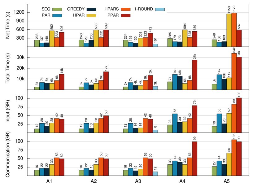
(a) Absolute values.

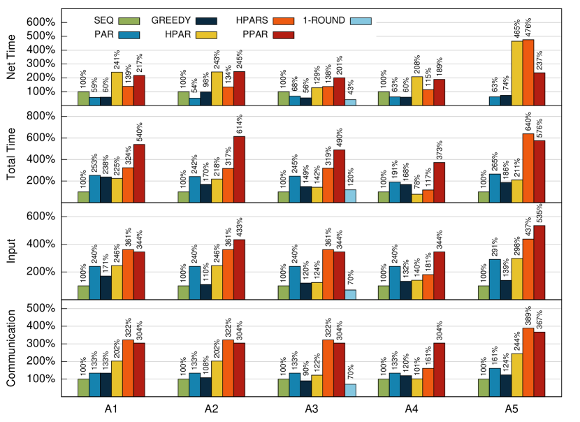
(b) Values relative to SEQ.

Figure 3: Results for evaluating the BSGF queries using different strategies.

Table 2 lists the type of BSGF queries used in this section. Figures 3 & 4 show the results that are discussed next.

Sequential vs. Parallel

We first compare sequential and parallel evaluation of queries A1–A5 to highlight the major differences between sequential and parallel query plans and to illustrate the effect of grouping. In particular, we consider three evaluation strategies in Gumbo: (i) evaluating all semi-joins sequentially by applying a semi-join to the output of the previous stage (SEQ), where the number of rounds depends on the number of semi-joins; (ii) using the 2-round strategy with algorithm Greedy-BSGF (GREEDY); and, (iii) a more naive version of GREEDY where no grouping occurs, i.e., every semi-join is evaluated separately in parallel (PAR). As semi-join algorithms in MR have not received significant attention, we choose to compare with the two extreme approaches: no parallelization (SEQ) and parallelization without grouping (PAR). Relative improvements of PAR and GREEDY w.r.t. SEQ are shown in Figure 3(b).

We find that both PAR and GREEDY result in lower net times. In particular, we see average improvements of 39% and 31% over SEQ, respectively. On the other hand, the total times for PAR are much higher than for SEQ: 132% higher on average. This is explained by the increase in both input and communication bytes, whereas the data size can be reduced after each step in the sequential evaluation. For GREEDY, total times vary depending on the structure of the query. Total times are significantly reduced for queries where conditional atoms share join keys and/or relation names. This effect is most obvious for queries A1, A2 and A5 where we oberve reductions in net time of 30%, 29% and 30%, respectively, w.r.t. PAR.

For query A3, all conditional atoms have the same join key, making 1-round (1-ROUND, see Section 5.1) evaluation possible. This further reduces the total and net time to only 49% and 63% of those of PAR, respectively.

Hive & Pig

We now examine parallel query evaluation in Pig and Hive and show that Gumbo outperforms both systems for BSGF queries. For this test, we implement the 2-round query plans of Section 4.4 directly in Pig and Hive. For Hive, we consider two evaluation strategies: one using Hive’s left-outer-join operations (HPAR) and one using Hive’s semi-join operations (HPARS). For Pig, we consider one strategy that is implemented using the COGROUP operation (PPAR). We also studied sequential evaluation of BSGF queries in both systems but choose to omit the results here as both performed drastically worse than their Gumbo equivalent (SEQ) in terms of net and total time.

First, we find that HPAR lacks parallelization. This is caused by Hive’s restriction that certain join operations are executed sequentially, even when parallel execution is enabled. This leads to net times that are 238% higher on average, compared to PAR. Note that query A3 shows a better net time than the other queries. This is caused by Hive allowing grouping on certain join queries, effectively bringing the number of jobs (and rounds) down to 2.

Next, we find that HPARS performs better than HPAR in terms of net time but is still 126% higher on average than PAR. The lower net times w.r.t. HPAR are explained by Hive allowing parallel execution of semi-join operations, without allowing any form of grouping. This effectively makes HPAR the Hive equivalent of PAR. The high net times are caused by Hive’s higher average map and reduce input sizes.

Finally, Pig shows an average net time increase of 254%. This is mainly caused by the lack of reduction in intermediate data and in input bytes, together with input-based reducer allocation (1GB of map input data per reducer). For these queries, this leads to a low number of reducers, causing the average reduce time, and hence overall net time, to go up.

As the reported net times for Hive and Pig are much higher than for sequential evaluation in Gumbo (SEQ), we conclude that Pig and Hive, with default settings, are unfit for parallel evaluation of BSGF queries. For this reason we restrict our attention to Gumbo in the following sections.

Large Queries

Next, we compare the evaluation of two larger BSGF queries B1 and B2 from Table 2. The results are shown in Figure 4. Query B1 is a conjunctive BSGF query featuring a high number of atoms. Its structure ensures a deep sequential plan that results in a high net time for SEQ. We find that PAR only takes 22% of the net time, which shows that parallel query plans can yield significant improvements. Conversely, PAR takes up 261% more total time than SEQ, as the latter is more efficient in pruning the data at each step. Here, GREEDY is able to successfully parallelize query execution without sacrificing total time. Indeed, GREEDY exhibits a net time comparable to that of PAR and a total time comparable to that of SEQ.

Query B2 consists of a large boolean combination and is called the uniqueness query. This query returns the tuples that can be connected to precisely one of the conditional relations through a given attribute. The number of distinct conditional atoms is limited, and the disjunction at the highest level makes it possible to evaluate the four conjunctive subexpressions in parallel using SEQ. Still, we find that the net time of of PAR improves that of SEQ by 66%. As PAR only needs to calculate the result of four semi-join queries in its first round, we also find a reduction of 57% in total time. GREEDY further reduces both numbers.

Finally, for B2, a 1-round evaluation (1-ROUND, see Section 5.1) can be considered, as only one key is used for the conditional atoms. This evaluation strategy brings down both net and total time of SEQ by more than 80%.

Cost Model

As explained in Section 3.3, the major difference between our cost model and that of Wang et al. [35] (referred to as $\operatorname{\text{\it cost}}_{\mathit{gumbo}}$ and $\operatorname{\text{\it cost}}_{\mathit{wang}}$, respectively, from here onward) concerns identifying the individual map cost contributions of the input relations. For queries where the map input/output ratio differs greatly among the input relations, we notice a vast improvement for the GREEDY strategy. We illustrate this using the following query:

$$R(x,y,z,w){}\ltimes{} S_{1}(\bar{x}_{1},c)\land\ldots\land S_{1}(\bar{x}_{12},c)\land{}$$

$$S_{2}(\bar{x}_{1},c)\land\ldots\land S_{2}(\bar{x}_{12},c)\land{}$$

$$S_{3}(\bar{x}_{1},c)\land\ldots\land S_{3}(\bar{x}_{12},c)\land{}$$

$$S_{4}(\bar{x}_{1},c)\land\ldots\land S_{4}(\bar{x}_{12},c),$$

where $\bar{x}_{1},\ldots,\bar{x}_{12}$ are all distinct keys and $c$ is a constant that filters out all tuples from $S_{1},\ldots,S_{4}$. The results for evaluating this query using GREEDY with $\operatorname{\text{\it cost}}_{\mathit{gumbo}}$ and $\operatorname{\text{\it cost}}_{\mathit{wang}}$ are unmistakable: $\operatorname{\text{\it cost}}_{\mathit{gumbo}}$ provides a 43% reduction in total time and a 71% reduction in net time. The explanation is that $\operatorname{\text{\it cost}}_{\mathit{wang}}$ does not discriminate between different input relations, it averages out the intermediate data and therefore fails to account for the high number of map-side merges and the accompanying increase in both total and net time.

For queries A1–A5 and B1–B2, where input relations have a contribution to map output that is proportional to their input size, we find that both cost models behave similarly. When comparing two random jobs, the cost models correctly identify the highest cost job in 72.28% ($\operatorname{\text{\it cost}}_{\mathit{gumbo}}$) and 69.37% of the cases ($\operatorname{\text{\it cost}}_{\mathit{wang}}$). Hence, we find that $\operatorname{\text{\it cost}}_{\mathit{gumbo}}$ provides a more robust cost estimation as it can isolate input relations that have a non-proportional contribution to the map output, while it automatically resorts to $\operatorname{\text{\it cost}}_{\mathit{wang}}$ in the case of an equal contribution.

Conclusion

We conclude that parallel evaluation effectively lowers net times, at the cost of higher total times. GREEDY, backed by an updated cost model, successfully manages to bring down total times of parallel evaluation, especially in the presence of commonalities among the atoms of BSGF queries. For larger queries, total times similar to SEQ are obtained. Finally, Gumbo outperforms Pig and Hive in all aspects when it comes to parallel evaluation of BSGF queries.

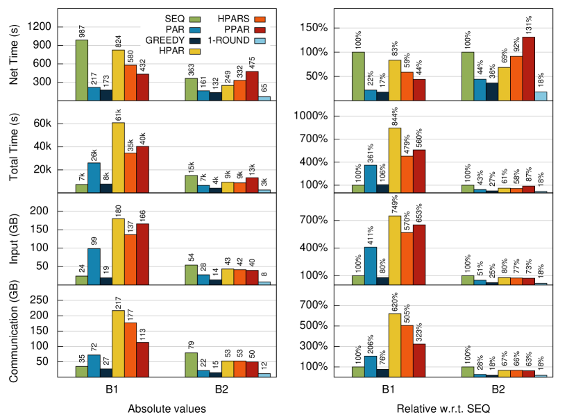
Figure 4: Large BSGF queries.

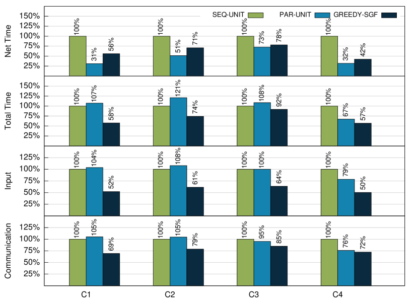
Figure 5: SGF results, values relative to SEQUNIT.

(a) Query Set C1

(b) Query Set C2

(c) Query C3

(d) Query C4

Figure 6: The queries used in the SGF experiment. Each node represents one BSGF subquery ($\bar{x}=x,y,z,w)$.

5.3 SGF Queries

In this section, we show that the algorithm Greedy-SGF succeeds in lowering total time while avoiding significant increase in net time. Figure 6 gives an overview of the type of queries that are used. Results are depicted in Figure 5. Note that these queries all exhibit different properties. Queries C1 and C2 both contain a set of SGF queries where a number of atoms overlap. Query C3 is a complex query that contains a multitude of different atoms. Finally, Query C4 consists of two levels and many overlapping atoms.

We consider the following evaluation strategies in Gumbo: (i) sequentially, i.e., one at a time, evaluating all BSGF queries in a bottom-up fashion (SEQUNIT); (ii) evaluating all BSGF queries in a bottom-up fashion level by level where queries on the same level are executed in parallel (PARUNIT); and, (iii) using the greedily computed topological sort combined with Greedy-BSGF (Greedy-SGF); Note that in SEQUNIT and PARUNIT all semi-joins are evaluated in separate jobs. For all tests conducted here, we found that Greedy-SGF yields multiway topological sorts that are identical to the optimal topological sort (computed trough brute-force methods); hence, we omit the results for the optimal plans.

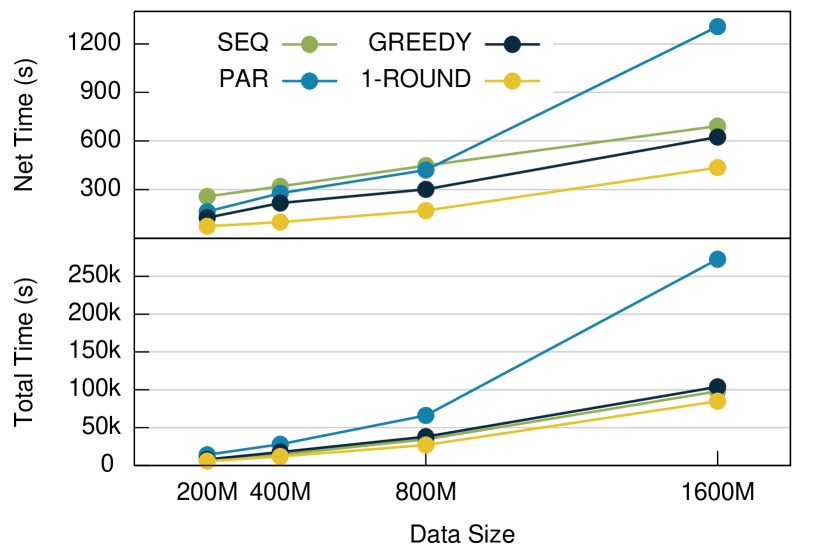
(a) Varying data size (10 nodes).

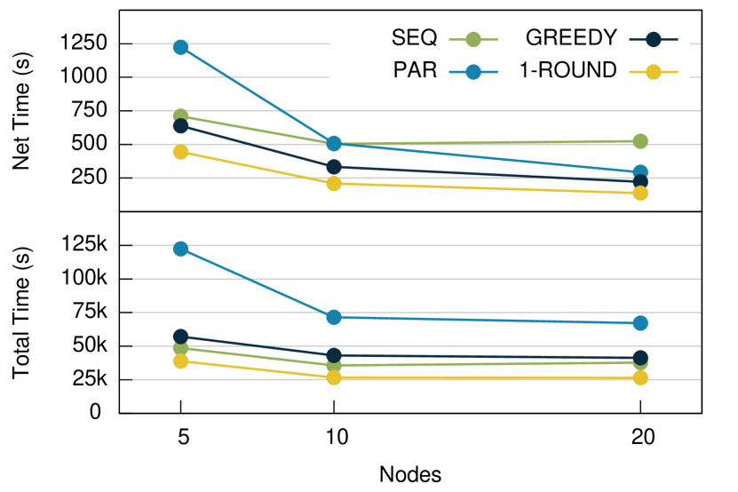
(b) Varying cluster size (800M tuples).

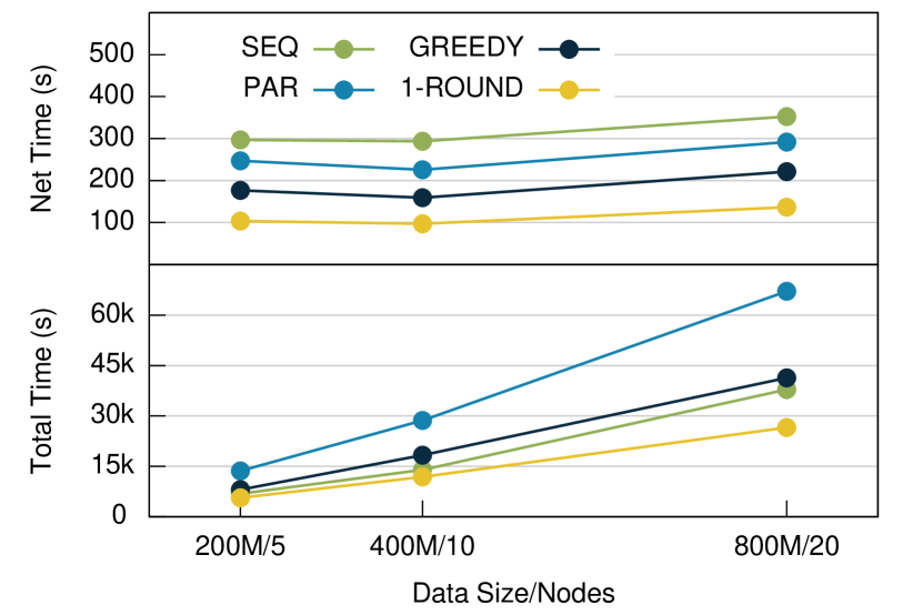
(c) Varying data and cluster size.

Figure 7: Results for system characteristics tests for Gumbo.

Similar to our observations for BSGF queries, we find that full sequential evaluation (SEQUNIT) results in the largest net times. Indeed, PARUNIT exhibits 55% lower net times on average. We also observe that PARUNIT exhibits significantly larger total times than SEQUNIT for queries C1 and C2, while this is not the case for C3 and C4. The reason is that for C3 and C4, queries on the same level still share common characteristics, leading to a lower number of distinct semi-joins.

For Greedy-SGF, we find that it exhibits net times that are, on average, 42% lower than SEQUNIT, while still being 29% higher than PARUNIT. The main reason for this is the fact that Greedy-SGF aims to minimize total time, and may introduce extra levels in the MR query plan to obtain this goal. Indeed, we find that total times are down 27% w.r.t. SEQUNIT, and 29% w.r.t. PARUNIT.

Finally, we note that the absolute savings in net time range from 115s to 737s for these queries, far outweighing the overhead cost of calculating the query plan itself, which typically takes around 10s (sampling included). Hence, we conclude that Greedy-SGF provides an evaluation strategy for SGF queries that manages to bring down the total time (and hence, the resource cost) of parallel query plans, while still exhibiting low net times when compared to sequential approaches.

5.4 System Characteristics

In this final experiment, we study the effect of growing data size, cluster size, query size, and selectivity. We choose queries similar to A3 to include the 1-ROUND strategy. Similar growth properties hold for the other query types.

Data & Cluster Size

Figures 7(a)-7(c) show the result of evaluating A3 using SEQ, PAR, GREEDY and 1-ROUND under the presence of variable data and cluster size. We summarize the most important observations:

1. in all scenarios, 1-ROUND performs best in terms of net and total time;

2. due to its lack of grouping, PAR needs a high number of mappers, which at some point exceeds the capacity of the cluster. This causes a large increase in net and total time, an effect that can be seen in Figure 7(a).

3. with regard to net time, adding more nodes is very effective for the parallel strategies PAR, GREEDY and 1-ROUND; in contrast, adding more nodes does not improve SEQ substantially after some point;

4. when scaling data and cluster size at the same time, all strategies are able to maintain their net times in the presence of an increasing total time.

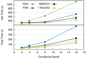
Figure 8: Varying the number of atoms.

Query Size

We consider a set of queries similar to A3, where the number of conditional atoms ranges from 2 to 16. Results are depicted in Figure 8. With regard to net time, we find that SEQ shows an increase in net time that is strongly related to the query size, while PAR, GREEDY and 1-ROUND are less affected. For total time, we observe the converse for PAR, as this strategy cannot benefit from the packing optimization in the same way as GREEDY and 1-ROUND can.

	Net time			Total time
	A1	A2	A3	A1	A2	A3
SEQ	10%	9%	8%	79%	95%	88%
PAR	33%	46%	69%	41%	47%	58%
GREEDY	23%	30%	13%	45%	57%	15%

Table 3: Increase in net and total time when changing selectivity from 0.1 to 0.9 for queries A1–A3.

Selectivity

For a conditional relation, we define its selectivity rate as the percentage of guard tuples it matches. We tested queries A1–A3 for selectivity rates 0.1 (high selectivity), 0.3, 0.5, 0.7 and 0.9 (low selectivity). The increase in net time and total time between selectivity rates 0.1 and 0.9 is summarized in Table 3. In general, we find that the selectivity has the most influence on the net times of PAR and GREEDY, and on the total times of SEQ. Finally, we observe that the filtering characteristics of SEQ disappear in the presence of low selectivity data, causing total times to become comparable to GREEDY for queries where packing is possible, such as A3. This can be explained by GREEDY being less sensitive to selectivity for queries where conditional atoms share a common join key, making an effective compression of intermediate data possible through packing.

6 Discussion

We have shown that naive parallel evaluation of semi-join and (B)SGF queries can greatly reduce the net time of query execution, but, as expected, generally comes at a cost of an increased total time. We presented several methods that aim to reduce the total cost (total time) of parallel MR query plans, while at the same time avoiding a high increase in net time. We proposed a two-tiered strategy for selecting the optimal parallel MR query plan for an SGF query in terms of total cost. As the general problem was proven to be NP-hard, we devised a two-tiered greedy approach that leverages on the existing technique of grouping MR jobs together based on a cost-model. The greedy approach was shown to be effective for evaluating (B)SGF queries in practice through several experiments using our own implementation called Gumbo. For certain classes of queries, our approach makes it even possible to evaluate (B)SGF queries in parallel with a total time similar to that of sequential evaluation. We also showed that the profuse number of optimizations that are offered in Gumbo allow it to outperform Pig and Hive in several aspects.

We remark that the techniques introduced in this paper generalize to any map/reduce framework (as, e.g., [37]) given an appropriate adaptation of the cost model.

Even though the algorithms in this paper do not directly take skew into account, the presented framework can readily be adapted to do so when information on so-called heavy hitters is available or can be computed at the expense of an additional round (see, e.g., [21, 29, 33, 31]).

Acknowledgment

The third author was supported in part by grant no. NTU-ERP-105R89082D and the Ministry of Science and Technology Taiwan under grant no. 104-2218-E-002-038. The computational resources and services used in this work were provided by the VSC (Flemish Supercomputer Center), funded by the Research Foundation - Flanders (FWO) and the Flemish Government – department EWI. We thank Jan Van den Bussche and Jelle Hellings for inspiring discussions and Geert Jan Bex for assistance with cluster setup.

Appendix A Proof of Theorem 2

In order to prove Theorem 2, we consider a more general problem. The same technique can then be used to prove the original theorem. We define the optimization problem Subset Cost-Opt that takes as input a set $S$ and a cost function $w:2^{|S|}\rightarrow\mathbb{N}$, and constructs a partition $\mathcal{S}=\{S_{1},\ldots,S_{n}\}$ of $S$ such that $\sum_{S_{i}\in\mathcal{S}}w(S_{i})$ is minimized. The decision version of Subset Cost-Opt, denoted by Subset Cost, corresponds to deciding, for a given positive integer $k$, whether there exists a partition $\mathcal{S}=\{S_{1},\ldots,S_{n}\}$ of $S$ such that $\sum_{i}^{n}w(S_{i})=k$. We now prove the NP-completeness of Subset Cost.

Theorem 3.

The Subset Cost problem is NP-complete.

Proof.

The problem is clearly in NP, as a given solution can be verified in polynomial time. We prove that this problem is NP-complete by a providing a polynomial time reduction from the Subset Sum problem, which consists of deciding, for given an integer $k$ and a set of positive integers $A$, whether there exists a set $B\subseteq A$ such that $\sum_{b\in B}b=k$. This problem is NP-complete [20].

The reduction is as follows. Given an instance of the subset sum problem, i.e., a set of integers $A$ and an integer $k$, we construct the following instance of Subset Cost: The set of items $S$ equals $A\cup\{\circ\}$, where $\circ$ is an element not present in $A$, and the cost function $w:2^{S}\to\mathbb{S}$ is defined as

$$w(X)=\begin{cases}\gamma&\mbox{if}\ \circ\in X\\ \sum_{a\in X}a&\mbox{otherwise}\\ \end{cases}$$ (11)

Here, $\gamma$ is an arbitrary constant. Intuitively, $w$ takes the sum of all items in a given set, except when the set contains the special item $\circ$. In that case, the value will be a fixed number $\gamma$.

In the remainder of this proof, we show that there exists a $B\subseteq A$ such that $\sum_{b\in B}b=k$ iff there exists a partition $\mathcal{S}=\{S_{1},\ldots,S_{n}\}$ of $S$ such that $\sum_{i}^{n}w(S_{i})=k+\gamma$.

Suppose there exists a partition $\mathcal{S}=\{S_{1},\ldots,S_{n}\}$ of $S$ such that $\sum_{i}^{n}w(S_{i})=k+\gamma$. Now, select the element of the partition that contains $\circ$, say $S_{\circ}$, and remove it from the partition to obtain a partition $\mathcal{S}^{\prime}$ for $S\setminus S_{\circ}$. Now, let $B=\bigcup\mathcal{S}^{\prime}$ and note that $B\subseteq A$. Clearly, the sum of the elements in $B$ equals $k+\gamma-\gamma=k$, as the cost of the removed element equals $\gamma$ by Equation (11). Hence, $B$ is a $k$-cost subset of $A$.

Suppose there exists a $B\subseteq A$ such that $\sum_{b\in B}b=k$. Consider the partition $\mathcal{S}=\{B,C\}$ of $S$, where $C=(A\setminus B)\cup\{\circ\}$. As $w(B)=k$ and $w(C)=\gamma$, we have a total cost of $k+\gamma$. ∎

We conclude this section by providing a proof for Theorem 2. Consider the decision version of SGF-Opt, which we’ll denote by SGF: for a DAG of BSGF queries $\mathcal{G}_{Q}$ and a positive integer $k$ determine whether there exists a multiway topological sort $\mathcal{F}$ of $\mathcal{G}_{Q}$ with $\operatorname{\text{\it cost}}(\mathcal{F})=k$.

Theorem 4.

The SGF problem is NP-complete.

Proof.

We can verify a solution for this problem in the following way: given a multiway topological sort $\mathcal{F}$ and a positive integer $k$, we can calculate its total cost using Equation (10), i.e.,

$$\operatorname{\text{\it cost}}(\mathcal{F})\ =\ \sum_{i=1}^{k}\ \operatorname{\text{\it cost}}(\textsf{GOPT}(F_{i})),$$

and check whether it equals $k$. As the greedy algorithm Greedy-BSGF for GOPT runs in polynomial time, the total cost can be calculated in polynomial time as well and hence the problem is in NP.

We now provide a polynomial time reduction from Subset Sum to SGF. Given an instance of the Subset Sum problem consisting of a set of positive integers $A=\{a_{1},\ldots,a_{n}\}$ and a positive integer $k$, we construct the following instance for SGF. Let $R_{1},\ldots,R_{n},R^{\circ}$ be a set of binary relations containing no tuples, a set of relations $S_{1},\ldots,S_{n}$ be a set of binary relations where $|S_{i}|=a_{i}$, each tuple has a size of 1MB and every second field has value 0. Also, consider a set of BSGF queries $F=\{f_{1},\ldots,f_{n},f^{\circ}\}$, where $f_{i}$ equals $R_{i}(x_{i},y_{i})\ltimes S_{i}(x_{i},1)$ and

$$f^{\circ}=R^{\circ}(x,1)\ltimes R_{1}(x_{1},y_{1})\land\ldots\land R_{n}(x_{n},y_{n})\land S_{1}(x_{1},1)\land\ldots\land S_{n}(x_{1},1).$$

Notice that there are no dependencies between the queries. Finally, for the Hadoop system, we choose all I/O constants equal to 0, except $h_{r}=1$.

Using Equation (9) and our cost model, we obtain that the cost of calculating each individual BSGF query $f_{i}$ equals $a_{i}$:

$$\operatorname{\text{\it cost}}(\textsf{GOPT}(\{f_{i}\})) =\operatorname{\text{\it cost}}(\textsf{EVAL}(R_{i},\varphi_{C_{i}}))+\operatorname{\text{\it cost}}(\{f_{i}\})$$

$$=0+\operatorname{\text{\it cost}}_{\text{\it map}}(|f_{i}|,|f_{i}|)+\operatorname{\text{\it cost}}_{\text{\it red}}(|f_{i}|,|f_{i}|)$$

$$=0+h_{r}\cdot a_{i}+0$$

$$=a_{i}.$$

Note that the EVAL job has cost 0, as no output is provided by the MSJ job.

We also find that the cost of two jobs equals their individual sums, regardless whether or not they are grouped in the query plan provided by GOPT:

$$\operatorname{\text{\it cost}}(\textsf{GOPT}(\{f_{i},f_{j}\})) =a_{i}+a_{j}.$$

Finally, we note that GOPT will always group $f_{i}$ with $f^{\circ}$ as all relations of $f_{i}$ appear in $f^{\circ}$. This leads to a cost of:

$$\operatorname{\text{\it cost}}(\textsf{GOPT}(\{f_{i},f^{\circ}\})) =\gamma,$$

where $\gamma=\sum_{i=1}^{n}a_{i}$.

Let $\mathcal{G}_{F}$ be the dependency graph that has nodes $F$ and no edges (as there are no query dependencies). Now, there exists a multiway topological sort for $\mathcal{G}_{F}$ of cost $k+\gamma$ iff there exists a $B\subseteq A$ such that $\sum_{b\in B}b=k$.

Observe that the cost function behaves completely analogous to the one used in the proof of Theorem 3. Hence, the same reasoning can now be applied to complete the proof. ∎

Appendix B Hadoop Settings & Cost Model Constants

Table 4 lists the settings for the Hadoop cluster that was utilized for our experiments. Table 5 shows the values that are used for the constants in the revised MapReduce cost model. The values were obtained using benchmark tests on system used for the experiments.

Hadoop Setting	Value
io.file.buffer.size	131072
dfs.replication	3
mapred.child.java.opts	-Xmx1024m
mapreduce.map.memory.mb	1280
mapreduce.reduce.memory.mb	1280
mapreduce.task.io.sort.mb	512
mapreduce.reduce.merge.inmem.threshold	0
mapreduce.reduce.input.buffer.percent	0.5
mapreduce.job.reduce.slowstart.completedmaps	1
mapred.map.tasks.speculative.execution	false
mapred.reduce.tasks.speculative.execution	false
yarn.nodemanager.resource.memory-mb	49152
yarn.scheduler.minimum-allocation-mb	4096
yarn.scheduler.maximum-allocation-mb	49152
yarn.nodemanager.resource.cpu-vcores	10

Table 4: Hadoop settings used in the experiments.

Constant	Description	Value
$l_{r}$	local disk read cost (per MB)	0.03
$l_{w}$	local disk write cost (per MB)	0.085
$h_{r}$	hdfs read cost (per MB)	0.15
$h_{w}$	hdfs write cost (per MB)	0.25
$t$	transfer cost (per MB)	0.017
$D$	external sort merge factor	10
$\mathit{buf}_{\text{\it map}}$	map task buffer limit (in MB)	409MB
$\mathit{buf}_{\text{\it red}}$	reduce task buffer limit (in MB)	512MB

Table 5: Description of constants used in the cost model.

References

- [1] S. Abiteboul, R. Hull, and V. Vianu. Foundations of Databases. Addison-Wesley, 1995.
- [2] F. Afrati, M. Joglekar, C. Ré, S. Salihoglu, and J. Ullman. GYM: A multiround join algorithm in mapreduce. CoRR, abs/1410.4156, 2014.
- [3] F. Afrati, A. D. Sarma, S. Salihoglu, and J. Ullman. Upper and lower bounds on the cost of a map-reduce computation. In VLDB, pages 277–288, 2013.
- [4] F. Afrati and J. Ullman. Optimizing multiway joins in a map-reduce environment. IEEE Trans. Knowl. Data Eng., 23(9):1282–1298, 2011.
- [5] F. Afrati, J. Ullman, and A. Vasilakopoulos. Handling skew in multiway joins in parallel processing. CoRR, abs/1504.03247, 2015.
- [6] H. Andreka, J. van Benthem, and I. Nemeti. Modal languages and bounded fragments of predicate logic. Journal of Philosophical Logic, 27(3):217–274, 1998.
- [7] P. Beame, P. Koutris, and D. Suciu. Communication steps for parallel query processing. In PODS, pages 273–284, 2013.
- [8] P. Beame, P. Koutris, and D. Suciu. Skew in parallel query processing. In PODS, pages 212–223, 2014.
- [9] P. Bernstein and D. Chiu. Using semi-joins to solve relational queries. J. ACM, 28(1):25–40, 1981.
- [10] P. Bernstein and N. Goodman. Power of natural semijoins. SIAM Journal on Computing, 10(4):751–771, 1981.
- [11] P. A. Bernstein and N. Goodman. The power of inequality semijoins. Inf. Syst., 6(4):255–265, 1981.
- [12] S. Blanas et al. A comparison of join algorithms for log processing in MapReduce. SIGMOD, pages 975–986, 2010.
- [13] S. Chaudhuri. An overview of query optimization in relational systems. In PODS, pages 34–43, 1998.
- [14] S. Chu, M. Balazinska, and D. Suciu. From theory to practice: Efficient join query evaluation in a parallel database system. In SIGMOD, pages 63–78, 2015.
- [15] J. Daenen, F. Neven, and T. Tan. Gumbo: Guarded fragment queries over big data. In EDBT, pages 521–524, 2015.
- [16] J. Daenen and T. Tan. Gumbo v0.4, May 2016. http://dx.doi.org/10.5281/zenodo.51517.
- [17] J. Dean and S. Ghemawat. MapReduce: Simplified data processing on large clusters. Commun. ACM, 51(1):107–113, 2008.
- [18] M. Elseidy, A. Elguindy, A. Vitorovic, and C. Koch. Scalable and adaptive online joins. In VLDB, pages 441–452, 2014.
- [19] J. Flum, M. Frick, and M. Grohe. Query evaluation via tree-decompositions. J. ACM, 49(6):716–752, 2002.
- [20] M. R. Garey and D. S. Johnson. Computers and Intractability: A Guide to the Theory of NP-Completeness. W. H. Freeman & Co., New York, NY, USA, 1979.
- [21] A. Gates, J. Dai, and T. Nair. Apache pig’s optimizer. IEEE Data Engineering Bulletin, 36(1):34–45, 2013.
- [22] E. Grädel. Description logics and guarded fragments of first order logic. In Description Logics, 1998.
- [23] Y. Ioannidis. Query optimization. ACM Computing Survey, 28(1):121–123, 1996.
- [24] P. Koutris and D. Suciu. Parallel evaluation of conjunctive queries. In PODS, 2011.
- [25] D. Leinders, M. Marx, J. Tyszkiewicz, and J. Van den Bussche. The semijoin algebra and the guarded fragment. Journal of Logic, Language and Information, 14:331–343, 2005.
- [26] T. Nykiel, M. Potamias, C. Mishra, G. Kollios, and N. Koudas. MRShare: Sharing across multiple queries in mapreduce. In VLDB, pages 494–505, 2010.
- [27] A. Okcan and M. Riedewald. Processing theta-joins using MapReduce. In SIGMOD, pages 949–960, 2011.
- [28] C. Olston, B. Reed, A. Silberstein, and U. Srivastava. Automatic optimization of parallel dataflow programs. In USENIX Annual Technical Conference, pages 267–273, 2008.
- [29] C. Olston, B. Reed, U. Srivastava, R. Kumar, and A. Tomkins. Pig latin: a not-so-foreign language for data processing. In SIGMOD, pages 1099–1110, 2008.
- [30] F. Picalausa, G. Fletcher, J. Hidders, and S. Vansummeren. Principles of guarded structural indexing. In ICDT, pages 245–256, 2014.
- [31] S. R. Ramakrishnan, G. Swart, and A. Urmanov. Balancing reducer skew in mapreduce workloads using progressive sampling. In SoCC, page 16. ACM, 2012.
- [32] Y. Tao, W. Lin, and X. Xiao. Minimal mapreduce algorithms. In SIGMOD, pages 529–540, 2013.
- [33] A. Thusoo, J. S. Sarma, N. Jain, Z. Shao, P. Chakka, N. Zhang, S. Anthony, H. Liu, and R. Murthy. Hive - a petabyte scale data warehouse using hadoop. In ICDE, pages 996–1005, 2010.
- [34] M. Vardi. Why is modal logic so robustly decidable? In DIMACS Workshop on Descriptive Complexity and Finite Models, pages 149–184, 1996.
- [35] G. Wang and C.-Y. Chan. Multi-query optimization in mapreduce framework. In VLDB, pages 145–156, 2013.
- [36] T. White. Hadoop - The Definitive Guide: Storage and Analysis at Internet Scale. O’Reilly, 2015.
- [37] R. Xin, J. Rosen, M. Zaharia, M. Franklin, S. Shenker, and I. Stoica. Shark: SQL and rich analytics at scale. In SIGMOD, pages 13–24, 2013.
- [38] M. Yannakakis. Algorithms for acyclic database schemes. In VLDB, pages 82–94, 1981.