Magic wavelengths, matrix elements, polarizabilities, and lifetimes of Cs

Abstract

Motivated by recent interest in their applications, we report a systematic study of Cs atomic properties calculated by a high-precision relativistic all-order method. Excitation energies, reduced matrix elements, transition rates, and lifetimes are determined for levels with principal quantum numbers $n\leq 12$ and orbital angular momentum quantum numbers $l\leq 3$. Recommended values and estimates of uncertainties are provided for a number of electric-dipole transitions and the electric dipole polarizabilities of the $ns$, $np$, and $nd$ states. We also report a calculation of the electric quadrupole polarizability of the ground state. We display the dynamic polarizabilities of the $6s$ and $7p$ states for optical wavelengths between 1160 nm and 1800 nm and identify corresponding magic wavelengths for the $6s-7p_{1/2}$, $6s-7p_{3/2}$ transitions. The values of relevant matrix elements needed for polarizability calculations at other wavelengths are provided.

I Introduction

Cs atoms are used in a wide range of applications including atomic clocks and realization of the second Heavner et al. (2014); Jefferts et al. (2014), the most precise low-energy test of the Standard Model of the electroweak interactions Porsev et al. (2009), search for spatiotemporal variation of fundamental constants Huntemann et al. (2014), study of degenerate quantum gases Clark et al. (2015), qubits of quantum information systems Wang et al. (2015), search for the electric-dipole moment of the electron Tang et al. (2015), atom interferometry Hamilton et al. (2015), atomic magnetometry Patton et al. (2014), and tests of Lorentz invariance Wolf et al. (2006). As a result, accurate knowledge of Cs atomic properties, in particular electric-dipole matrix elements, lifetimes, polarizabilities, and magic wavelengths became increasingly important. While a number of $6s-np$ and $7s-np$ transitions have been studied in detail owing to their importance to test of the Standard Model Porsev et al. (2009), recent applications require reliable values of many other properties.

Many of the applications listed above involve optically trapped Cs atoms. The energy levels of atoms trapped in a light field are generally shifted by a quantity that is proportional to their frequency-dependent polarizability Mitroy et al. (2010). It is often beneficial to minimize the resulting ac Stark shift of transitions between different levels, for example in cooling or trapping applications. At a “magic wavelength”, which was first used in atomic clock applications Katori et al. (1999); Ye et al. (1999), the ac Stark shift of a transition is zero. Magic wavelengths for $6s-7p$ transitions are of potential use for state-insensitive cooling and trapping and have not been previously calculated. Similar $2s-3p$ and $4s-5p$ transitions have been recently used in ⁶Li Duarte et al. (2011) and ⁴⁰K McKay et al. (2011), respectively, as alternatives to conventional cooling with the $2s-2p$ and $4s-4p$ transitions.

Here we report an extensive study of a variety of Cs properties of experimental interest. We use several variants of the relativistic high-precision all-order (linearized coupled-cluster) method Safronova and Johnson (2008) to critically evaluate the accuracy of our calculations and provide recommended values with associated uncertainties. Atomic properties of Cs are evaluated for $ns$, $np$, $nd$, and $nf$ states with $n\leq 12$ . Excitation energies and lifetimes are calculated for the lowest 53 excited states. The reduced electric-dipole matrix elements, line strengths, and transition rates are determined for allowed transitions between these levels. The static electric quadrupole polarizability is determined for the $6s$ level. Scalar and tensor polarizabilities of $(5-9)d$, $(6-9)p$, and $(7-10)s$ states of Cs are evaluated. The uncertainties of the final values are estimated for all properties.

As a result of these calculations, we are able to identify the magic wavelengths for the $6s-7p_{1/2}$ and $6s-7p_{3/2}$ transitions in the 1160 nm and 1800 nm wavelength range.

Table 1: Recommended values of the reduced electric-dipole matrix elements $D$ in cesium in atomic units. Uncertainties are given in parenthesis. Absolute values are given.

Transition	D	Transition	D	Transition	D	Transition	D	Transition	D
$7s-6p_{1/2}$	4.24(1)	$6p_{1/2}-7d_{3/2}$	2.05(2)	$5d_{3/2}-6p_{1/2}$	7.1(1)	$6d_{3/2}-6p_{1/2}$	4.23(7)	$5d_{3/2}-7f_{5/2}$	1.73(1)
$7s-6p_{3/2}$	6.48(2)	$6p_{3/2}-7d_{3/2}$	0.976(0)	$5d_{3/2}-7p_{1/2}$	2.3(4)	$6d_{3/2}-7p_{1/2}$	17.99(4)	$5d_{3/2}-8f_{5/2}$	1.34(1)
$7s-7p_{1/2}$	10.31(4)	$6p_{3/2}-7d_{5/2}$	2.89(3)	$5d_{3/2}-8p_{1/2}$	0.63(5)	$6d_{3/2}-8p_{1/2}$	5.0(2)	$5d_{5/2}-6f_{5/2}$	0.644(6)
$7s-7p_{3/2}$	14.32(6)	$6p_{3/2}-10d_{5/2}$	0.979(6)	$5d_{3/2}-9p_{1/2}$	0.34(2)	$6d_{3/2}-9p_{1/2}$	1.56(2)	$5d_{5/2}-6f_{7/2}$	2.88(3)
$7s-8p_{1/2}$	0.914(27)	$6p_{3/2}-11d_{5/2}$	0.782(5)	$5d_{3/2}-10p_{1/2}$	0.22(1)	$6d_{3/2}-10p_{1/2}$	0.85(2)	$5d_{5/2}-7f_{5/2}$	0.468(3)
$7s-8p_{3/2}$	1.620(35)	$7p_{1/2}-6d_{3/2}$	17.99(4)	$5d_{3/2}-11p_{1/2}$	0.164(9)	$6d_{3/2}-11p_{1/2}$	0.56(1)	$5d_{5/2}-7f_{7/2}$	2.10(1)
$7s-9p_{1/2}$	0.349(10)	$7p_{3/2}-6d_{3/2}$	8.07(2)	$5d_{3/2}-12p_{1/2}$	0.128(7)	$6d_{3/2}-12p_{1/2}$	0.415(8)	$6d_{3/2}-4f_{5/2}$	24.62(9)
$7s-9p_{3/2}$	0.680(14)	$7p_{3/2}-6d_{5/2}$	24.35(6)	$5d_{3/2}-6p_{3/2}$	3.19(7)	$6d_{3/2}-6p_{3/2}$	2.09(3)	$6d_{5/2}-4f_{5/2}$	6.60(2)
$7s-10p_{1/2}$	0.191(6)	$7p_{3/2}-10d_{3/2}$	0.680(6)	$5d_{3/2}-7p_{3/2}$	0.9(2)	$6d_{3/2}-7p_{3/2}$	8.07(2)	$6d_{5/2}-4f_{7/2}$	29.5(1)
$7s-10p_{3/2}$	0.396(9)	$7p_{3/2}-10d_{5/2}$	2.02(2)	$5d_{3/2}-8p_{3/2}$	0.26(3)	$6d_{3/2}-8p_{3/2}$	1.98(7)	$7d_{3/2}-5f_{5/2}$	43.4(2)
$7s-11p_{1/2}$	0.125(4)	$7p_{3/2}-11d_{5/2}$	1.55(1)	$5d_{3/2}-9p_{3/2}$	0.14(1)	$6d_{3/2}-9p_{3/2}$	0.633(9)	$7d_{5/2}-5f_{5/2}$	11.66(5)
$7s-11p_{3/2}$	0.270(7	$8p_{1/2}-7d_{3/2}$	32.0(1)	$5d_{3/2}-10p_{3/2}$	0.091(7)	$6d_{3/2}-10p_{3/2}$	0.346(7)	$7d_{5/2}-5f_{7/2}$	52.2(2)
$8s-7p_{1/2}$	9.31(2)	$8p_{3/2}-7d_{3/2}$	14.35(5)	$5d_{3/2}-11p_{3/2}$	0.067(5)	$6d_{3/2}-11p_{3/2}$	0.230(5)	$8d_{3/2}-6f_{5/2}$	65.2(5)
$8s-7p_{3/2}$	14.07(7)	$8p_{3/2}-7d_{5/2}$	43.2(1)	$5d_{3/2}-12p_{3/2}$	0.052(4)	$6d_{3/2}-12p_{3/2}$	0.169(4)	$8d_{5/2}-6f_{5/2}$	17.5(1)
$8s-8p_{1/2}$	17.78(6)	$9p_{1/2}-8d_{3/2}$	49.3(1)	$5d_{5/2}-6p_{3/2}$	9.7(2)	$6d_{5/2}-6p_{3/2}$	6.13(9)	$8d_{5/2}-6f_{7/2}$	78.4(6)
$8s-8p_{3/2}$	24.56(9)	$9p_{3/2}-8d_{3/2}$	22.14(7)	$5d_{5/2}-7p_{3/2}$	2.8(5)	$6d_{5/2}-7p_{3/2}$	24.35(6)	$9d_{3/2}-7f_{5/2}$	90.5(9)
$9s-7p_{1/2}$	1.96(2)	$9p_{3/2}-8d_{5/2}$	66.6(2)	$5d_{5/2}-8p_{3/2}$	0.80(7)	$6d_{5/2}-8p_{3/2}$	6.2(2)	$9d_{5/2}-7f_{5/2}$	24.4(2)
$9s-8p_{1/2}$	16.06(4)	$10p_{1/2}-9d_{3/2}$	70.0(1)	$5d_{5/2}-9p_{3/2}$	0.43(3)	$6d_{5/2}-9p_{3/2}$	1.97(3)	$9d_{5/2}-7f_{7/2}$	108.9(0)
$9s-8p_{3/2}$	24.13(5)	$10p_{3/2}-9d_{3/2}$	31.45(8)	$5d_{5/2}-10p_{3/2}$	0.28(2)	$6d_{5/2}-10p_{3/2}$	1.07(2)	$10d_{5/2}-6f_{5/2}$	2.14(2)
$9s-9p_{1/2}$	27.10(8)	$10p_{3/2}-9d_{5/2}$	94.5(2)	$5d_{5/2}-11p_{3/2}$	0.21(1)	$6d_{5/2}-11p_{3/2}$	0.71(1)	$10d_{5/2}-6f_{7/2}$	9.56(8)
$9s-9p_{3/2}$	37.3(1)	$11p_{1/2}-10d_{3/2}$	94.1(2)	$5d_{5/2}-12p_{3/2}$	0.16(1)	$6d_{5/2}-12p_{3/2}$	0.53(1)	$10d_{5/2}-8f_{5/2}$	32.1(3)
$10s-7p_{1/2}$	0.999(9)	$11p_{3/2}-10d_{3/2}$	42.29(9)	$7d_{3/2}-6p_{1/2}$	2.05(2)	$7d_{5/2}-6p_{3/2}$	2.89(3)	$10d_{5/2}-8f_{7/2}$	143(1)
$10s-8p_{1/2}$	3.15(3)	$11p_{3/2}-10d_{5/2}$	127.0(2)	$7d_{3/2}-7p_{1/2}$	6.6(2)	$7d_{5/2}-7p_{3/2}$	9.6(3)	$11d_{5/2}-7f_{5/2}$	3.08(3)
$10s-9p_{1/2}$	24.50(5)	$12p_{1/2}-11d_{3/2}$	121.6(2)	$7d_{3/2}-8p_{1/2}$	32.0(1)	$7d_{5/2}-8p_{3/2}$	43.2(1)	$11d_{5/2}-7f_{7/2}$	13.8(1)
$10s-9p_{3/2}$	36.69(8)	$12p_{3/2}-11d_{3/2}$	54.66(9)	$7d_{3/2}-9p_{1/2}$	9.0(2)	$7d_{5/2}-9p_{3/2}$	11.1(2)	$12d_{5/2}-8f_{5/2}$	4.21(4)
$11s-7p_{1/2}$	0.650(6)	$12p_{3/2}-11d_{5/2}$	164.1(2)	$7d_{3/2}-9p_{3/2}$	3.56(9)	$7d_{5/2}-10p_{3/2}$	3.6(1)	$12d_{5/2}-8f_{7/2}$	18.8(2)
$11s-8p_{1/2}$	1.56(1)	$12s-8p_{1/2}$	1.002(9)	$7d_{3/2}-6p_{3/2}$	0.976(0)	$7d_{3/2}-12p_{3/2}$	0.42(1)	$7d_{3/2}-8p_{3/2}$	14.35(5)
$11s-9p_{1/2}$	4.61(4)	$12s-9p_{1/2}$	2.24(2)	$7d_{3/2}-7p_{3/2}$	3.3(1)	$7d_{3/2}-10p_{1/2}$	2.86(8)	$7d_{5/2}-11p_{3/2}$	1.97(6)
$11s-9p_{3/2}$	6.29(6)	$13s-7p_{1/2}$	0.370(3)	$7d_{3/2}-10p_{3/2}$	1.16(4)	$7d_{3/2}-11p_{1/2}$	1.55(4)
$12s-7p_{1/2}$	0.474(5)	$13s-8p_{1/2}$	0.727(6)	$7d_{3/2}-11p_{3/2}$	0.64(2)	$7d_{3/2}-12p_{1/2}$	1.03(3)

II Previous Cs polarizability studies

In 2010, Mitroy et al. Mitroy et al. (2010) reviewed the theory and applications of atomic and ionic polarizabilities across the periodic table of the elements. The static and dynamic polarizabilities of Cs have increased in interest recently, as demonstrated by a number of experimental Robyr et al. (2014); Antypas and Elliott (2011); Kortyna et al. (2011); Zhao et al. (2011); Auzinsh et al. (2007); Ulzega et al. (2007); Gunawardena et al. (2007); Sieradzan et al. (2004); Amini and Gould (2003); Ospelkaus et al. (2003); Bennett and Wieman (1999); Yei et al. (1998); Cho et al. (1997) and theoretical Kamenski and Ovsiannikov (2014); Tang et al. (2014); Roberts et al. (2013); Derevianko et al. (2010); Dzuba et al. (2010); Mitroy et al. (2010); Kondratjev et al. (2010); Il’inova et al. (2009); Hofer et al. (2008); Iskrenova-Tchoukova et al. (2007); Ulzega et al. (2006); Porsev and Derevianko (2006); Safronova et al. (2006); Lim et al. (2005); Safronova and Clark (2004); Magnier and Aubert-Frécon (2002); Safronova et al. (1999); Lim et al. (1999); Xia et al. (1997); van Wijngaarden and Li (1994); Fuentealba and Reyes (1993) studies.

Safronova et al. Safronova et al. (2006) presented results of first-principles calculations of the frequency-dependent polarizabilities of all alkali-metal atoms for light in the wavelength range 300-1600 nm, with particular attention to wavelengths of common infrared lasers. High-precision study of Cs polarizabilities for a number of states was presented in Ref. Iskrenova-Tchoukova et al. (2007). Inconsistencies between $5d$ lifetimes and $6p$ polarizability measurements in Cs was investigated by Safronova and Clark Safronova and Clark (2004). The ab initio calculation of $6p$ polarizabilities were found to agree with experimental values Safronova and Clark (2004). An experimental and theoretical study of the $6d_{3/2}$ polarizability of cesium was reported by Kortyna et al. Kortyna et al. (2011). The scalar and tensor polarizabilities were determined from hyperfine-resolved Stark–shift measurements using two-photon laser-induced-fluorescence spectroscopy of an effusive beam. Auzinsh et al. Auzinsh et al. (2007) presented an experimental and theoretical investigation of the polarizabilities and hyperfine constants of $nd$ states in ¹³³Cs. Experimental values for the hyperfine constant $A$ were obtained from level-crossing signals of the $(7,9,10)d_{5/2}$ states of Cs and precise calculations of the tensor polarizabilities $\alpha_{2}$. The results of relativistic many-body calculations for scalar and tensor polarizabilities of the $(5-10)d_{3/2}$ and $(5-10)d_{5/2}$ states were presented and compared with measured values from the literature. Gunawardena et al. Gunawardena et al. (2007) presented results of a precise determination of the static polarizability of the $8s$ state of atomic cesium, carried out jointly through experimental measurements of the dc Stark shift of the $6s\rightarrow 8s$ transition using Doppler-free two-photon absorption and theoretical computations based on a relativistic all-order method.

III Electric-dipole matrix elements and lifetimes of cesium

We carried out several calculations using different methods of increasing accuracy: the lowest-order Dirac-Fock approximation (DF), second-order relativistic many-body perturbation theory (RMBPT), third-order RMBPT, and several variants of the linearized coupled-cluster (all-order) method. Comparing values obtained in different approximations allows us to evaluate the size of the higher-order correlations corrections beyond the third order and estimate some omitted classes of the high-order correlations correction. As a result, we can present recommended values of Cs properties and estimate their uncertainties. The RMBPT calculations are carried out using the method described in Ref. Johnon et al. (1996). A review of the all-order method, which involves summing series of dominant many-body perturbation terms to all orders, is given in Safronova and Johnson (2008). In the single-double (SD) all-order approach, single and double excitations of the Dirac-Fock orbitals are included. The SDpT all-order approach also includes classes of the triple excitations. Omitted higher excitations can also be estimated by the scaling procedure described in Safronova and Johnson (2008), which can be started from either SD or SDpT approximations. We carry out all four of such all-order computations, ab initio SD and SDpT and scaled SD and SDpT.

The removal energies for a large number of Cs states, calculated in various approximations are given in Table I of the Supplemental Material SM . The accuracy of the energy levels is a good general indicator of the overall accuracy of the method. The all-order ab initio SD and SDpT values for the ground state ionization potential differ from the experiment nis by 0.4% and 0.58% respectively. Final ab initio SDpT all-order energies are in excellent agreement with experiment, to 0.05-0.4% for all levels with the exception of the $5d$ states, where the difference is 1.3%-1.4%. The larger discrepancy with experiment for the $5d$ states is explained by significantly larger correlation corrections, 16% for the $5d_{3/2}$ state in comparison with only 7% for the $6p_{1/2}$ state. In the isoelectronic spectra of Ba⁺ and La²⁺, on the other hand, the correlation corrections of $5d$ and $6s$ states are comparable Safronova and Safronova (2011, 2014). Moreover, triple and higher excitations are significantly larger for the $5d$ states in comparison to all other states. For example, the difference of the SD and SDpT values is 398 cm^-1 for the $5d_{3/2}$ state and only 51 cm^-1 for the ground state. As a result, some properties of the $5d$ states are less accurate than the properties of the other states. The scaling procedure mentioned above is used to correct electric-dipole matrix elements involving $5d$ states for missing higher excitations.

Table 2: Recommended values of radiative lifetimes in nsec). Uncertainties are given in parenthesis and references are given in brackets. The values of lifetimes evaluated in the lowest-order DF approximation are given in column DF to illustrate the importance of the correlation corrections. Experimental and other theoretical values are listed in the two last columns.

Level	DF	Recomm.	Expt.	Other
$6p_{1/2}$	25.4	34.4(1.2)	34.934(94) Young et al. (1994)
$6p_{3/2}$	22.2	30.0(0.7)	30.460(38) Sell et al. (2011)
$5d_{3/2}$	600	966(34)	909(15) DiBerardino et al. (1998)	976 DiBerardino et al. (1998)
$5d_{5/2}$	847	1351(52)	1281(9)  DiBerardino et al. (1998)	1363  DiBerardino et al. (1998)
$7s_{1/2}$	45.3	48.4(0.2)	49(4)  Marek (1977a)	56  Marek (1977a)
$7p_{1/2}$	84	152(18)	155(4)  Ortiz and Campos (1981)	135  Ortiz and Campos (1981)
$7p_{3/2}$	77	128(10)	133(2) Ortiz and Campos (1981)	110  Ortiz and Campos (1981)
$6d_{3/2}$	153	61(2)	60.0(2.5) Marek and Ryschka (1979)	69.9 Marek and Ryschka (1979)
$6d_{5/2}$	138	61(2)	60.7(2.5) Marek and Ryschka (1979)	64.5 Marek and Ryschka (1979)
$8s_{1/2}$	87	93(1)	87(9)  Marek (1977b)	104  Marek (1977b)
$4f_{7/2}$	25	51(7)	40(6) Marek (1977a)	43 Marek (1977a)
$4f_{5/2}$	24	51(7)	40(6) Marek (1977a)	43 Marek (1977a)
$8p_{1/2}$	201	376(16)	307(14) Marek and Niemax (1976)
$8p_{3/2}$	186	320(11)	274(12) Marek and Niemax (1976)
$7d_{3/2}$	160	95(2)	89(1) Neil and Atkinson (1984)	107 Neil and Atkinson (1984)
$7d_{5/2}$	151	95(2)	89(1) Neil and Atkinson (1984)	107 Neil and Atkinson (1984)
$9s_{1/2}$	157	167(2)	159(3) Neil and Atkinson (1984)	177 Neil and Atkinson (1984)
$5f_{7/2}$	54	96(4)	97(6) Marek and Ryschka (1979)	76.8 Marek and Ryschka (1979)
$5f_{5/2}$	53	96(4)	95(6) Marek and Ryschka (1979)
$9p_{1/2}$	386	695(19)	575(35) Marek and Niemax (1976)
$9p_{3/2}$	360	606(16)	502(22) Marek and Niemax (1976)
$8d_{3/2}$	223	153(3)	141(2) Neil and Atkinson (1984)	168 Neil and Atkinson (1984)
$8d_{5/2}$	213	153(3)	145(3) Neil and Atkinson (1984)	168 Neil and Atkinson (1984)
$10s_{1/2}$	262	279(3)	265(4) Neil and Atkinson (1984)	293 Neil and Atkinson (1984)
$6f_{7/2}$	97	159(3)	149(8) Marek and Ryschka (1979)	123.8 Marek and Ryschka (1979)
$6f_{5/2}$	96	160(3)
$10p_{1/2}$	652	1132(29)	920(50) Sieradzan et al. (1979)
$10p_{3/2}$	610	1006(26)	900(40) Sieradzan et al. (1979)
$9d_{3/2}$	321	235(4)	218(3) Neil and Atkinson (1984)	257 Neil and Atkinson (1984)
$9d_{5/2}$	308	237(4)	217(4) Neil and Atkinson (1984)	257 Neil and Atkinson (1984)
$11s_{1/2}$	408	434(4)	403(4) Neil and Atkinson (1984)	455 Neil and Atkinson (1984)
$7f_{7/2}$	158	246(3)	229(15) Marek and Ryschka (1979)	189.2 Marek and Ryschka (1979)
$7f_{5/2}$	155	248(3)
$11p_{1/2}$	1012	1702(41)
$11p_{3/2}$	950	1538(37)
$10d_{3/2}$	454	348(6)	315(3) Neil and Atkinson (1984)	376 Neil and Atkinson (1984)
$10d_{5/2}$	439	350(3)	321(4) Neil and Atkinson (1984)	376 Neil and Atkinson (1984)
$12s_{1/2}$	602	642(6)	573(7) Neil and Atkinson (1984)	668 Neil and Atkinson (1984)
$8f_{7/2}$	238	361(20)
$8f_{5/2}$	234	363(6)	336(22) Marek and Ryschka (1979)	274.8 Marek and Ryschka (1979)
$12p_{1/2}$	1484	2430(55)
$12p_{3/2}$	1394	2218(52)
$11d_{3/2}$	626	492(8)	417(5) Neil and Atkinson (1984)	529 Neil and Atkinson (1984)
$11d_{5/2}$	605	496(5)	420(7) Neil and Atkinson (1984)	529 Neil and Atkinson (1984)
$13s_{1/2}$	846	901(8)	777(8) Neil and Atkinson (1984)	942 Neil and Atkinson (1984)
$9f_{7/2}$	340	506(23)	473(30) Marek and Ryschka (1979)	385.1 Marek and Ryschka (1979)
$9f_{5/2}$	335	511(26)
$12d_{3/2}$	794	663(24)	566(11) Neil and Atkinson (1984)	722 Neil and Atkinson (1984)
$12d_{5/2}$	768	661(29)	586(11)	722
$14s_{1/2}$	1033	1087(9)	1017(20) Neil and Atkinson (1984)	1282 Neil and Atkinson (1984)
$10f_{7/2}$	419	620(27)	646(35) Marek and Ryschka (1979)	521.1 Marek and Ryschka (1979)
$10f_{5/2}$	414	626(29)

III.1 Electric-dipole matrix elements

We calculated the 126 $ns-n^{\prime}p$ ($n=6-14$ and $n^{\prime}=6-12$), 168 $np-n^{\prime}d$ ($n=6-12$ and $n^{\prime}=5-12$), and 168 $nd-n^{\prime}f$ ($n=5-12$ and $n^{\prime}=4-10$) transitions. Table 1 reports those values that make significant contributions to the atomic lifetimes and polarizabilities calculated in the other sections. The absolute values are given in all cases in units of $a_{0}e$, where $a_{0}$ is the Bohr radius and $e$ is the elementary charge. More details of the matrix-element calculations, including the lowest-order values, are given in Supplemental Material SM .

Unless stated otherwise, we use the conventional system of atomic units, a.u., in which $e$, the electron mass $m_{\rm e}$, and the reduced Planck constant $\hbar$ have the numerical value 1, and the electric constant $\epsilon_{0}$ has the numerical value $1/(4\pi)$. Dipole polarizabilities $\alpha$ in a.u. have the dimension of volume, and their numerical values presented here are expressed in units of $a^{3}_{0}$. The atomic units for $\alpha$ can be converted to SI units via $\alpha/h$ [Hz/(V/m)²]=2.48832$\times 10^{-8}\alpha$ [a.u.], where the conversion coefficient is $4\pi\epsilon_{0}a^{3}_{0}/h$ and the Planck constant $h$ is factored out.

The estimated uncertainties of the recommended values are listed in parenthesis. The evaluation of the uncertainty of the matrix elements was described in detail in Safronova and Safronova (2011, 2012). It is based on four different all-order calculations mentioned in Section III: two ab initio all-order calculations with (SDpT) and without (SD) the inclusion of the partial triple excitations and two calculations that included semiempirical estimate of missing high-order correlation corrections starting from both ab initio calculations. The spread of these four values was used to estimate uncertainty in the final results for each transition based on the algorithm accounting for the importance of the specific dominant contributions. The largest values of the uncertainties in Table 1 are for the $5d-np$ transitions, ranging from 1.9% to to 10% for most cases resulting from larger correlation for the $5d$ states discussed above. The uncertainties are the largest (20%) for the $5d-7p$ transitions. Our final results and their uncertainties are used to calculate the recommended values of the lifetimes and polarizabilities discussed below.

III.2 Lifetimes

One of the first lifetime measurements in cesium was published by Gallagher Gallagher (1967). Level crossing measurement of lifetimes in Cs were presented by Schmieder and Lurio Schmieder and Lurio (1970). Using a pulsed dye laser and the method of delayed coincidence the lifetime of the $7p$, $8p$, and $9p$ levels were measured by Marek and Niemax Marek and Niemax (1976). The cascade Hanle–effect technique were used by Budos et al. Bulos et al. (1976) for the lifetime measurements of the $8s$ and $9s$ levels. Deech et al. Deech et al. (1977) reported results of the lifetime measurements made by time-resolved fluorescence from $ns$ and $nd_{3/2}$ states of Cs ($n=$8 to 14) over a range of vapour densities covering the onset of collisional depopulation. The same technique was used by Marek Marek (1977a) to find out the lifetimes for the $7s$, $5d$, and $4f$ levels. Radiative lifetimes of the $8s$, $9s$ and $7d$ levels of Cs were measured by Marek Marek (1977b) employing the method of delayed coincidences of cascade transitions to levels that cannot be directly excited by electronic dipole transitions from ground state. Alessandretti et al. Alessandretti et al. (1977) reported measurement of the $8s$-level lifetime in Cs vapor, using the two-photon $6s\rightarrow 8s$ transition. Marek and Ryschka Marek and Ryschka (1979) presented lifetime measurements of $5f$ - $11f$ levels of Cs using partially superradiant population. Ortiz and Campos Ortiz and Campos (1981) measured lifetimes of the $7p_{1/2}$ and $7p_{3/2}$ levels of Cs. Neil and Atkinson Neil and Atkinson (1984) reported the lifetimes of the $ns$ ($n$ = 9-15), $nd_{3/2}$. and $nd_{5/2}$ ($n=7-12$) levels with 1-2% accuracy. Lifetimes were measured by laser-induced fluorescence using two-photon excitation. Small differences between the lifetimes of the different fine-structure levels of each $nd$ state have been observed for the first time Neil and Atkinson (1984). Bouchiat et al. Bouchiat et al. (1992) reported measurement of the radiative lifetime of the cesium $5d_{5/2}$ level using pulsed excitation and delayed probe absorption. Sasso et al. Bouchiat et al. (1992) reported measurement of the radiative lifetimes and quenching of the cesium $5d$ levels. Measurement of the $5d_{5/2}$ lifetime was presented by Hoeling et al. Hoeling et al. (1996) and by DiBerardino et al. DiBerardino et al. (1998).

Table 3: Reduced quadrupole matrix elements $Q$ in a.u. and contributions to quadrupole polarizabilities of the $6s$ state of cesium in $a_{0}^{5}$. Uncertainties are given in parenthesis.

Contr.	$Q$	$\alpha^{E2}_{0}(6s)$
$5d_{3/2}$	33.62	3421(69)
$6d_{3/2}$	12.98	327(21)
$7d_{3/2}$	8.08	109(4)
$8d_{3/2}$	5.53	48(1)
$(9-26)d_{3/2}$		287(1)
$5d_{5/2}$	41.51	5183(88)
$6d_{5/2}$	15.26	452(28)
$7d_{5/2}$	9.64	157(6)
$8d_{5/2}$	6.64	70(2)
$(9-26)d_{5/2}$		379(1)
CORE		86(2)
Total		10521(118)

Precision lifetime measurements of the $6p$ states in atomic cesium were published in a number of papers by Tanner et al. Tanner et al. (1992), Rafac et al. Rafac et al. (1994), Young et al. Young et al. (1994), and Rafac et al. Rafac et al. (1999). The most accurate result was reported by Rafac et al. Rafac et al. (1994) with lifetimes for $6p_{1/2}$ (34.934$\pm$0.094 ns) and $6p_{3/2}$ (30.499$\pm$0.070 ns) states in atomic cesium obtained using the resonant diode-laser excitation of a fast atomic beam to produce those measurements. Recently, lifetime of the cesium $6p_{3/2}$ state was measured using ultrafast laser-pulse excitation and ionization. The result of Sell et al. Sell et al. (2011), $\tau(6p_{3/2})=30.460(38)$ ns with an uncertainty of 0.12%, is one of the most accurate lifetime measurements on record.

We calculated lifetimes of the $(7-14)s$, $(6-12)p$, $(5-12)d$, and $(4-10)f$ states in Cs using out final values of the matrix elements listed in Table 1 and experimental energies from  nis . The uncertainties in the lifetime values are obtained from the uncertainties in the matrix elements listed in Table 1. Since experimental energies are very accurate, the uncertainties in the lifetimes originate from the uncertainties in the matrix elements. We also included the lowest-order DF lifetimes $\tau^{{\rm DF}}$ to illustrate the size of the correlation effects, which can be estimated as the differences of the final and lowest-order values. We note that the correlation contributions are large, 5-60%, being 30-40% for most states.

Our results are compared with experiment and other theory. We note that the theoretical results in the “$\tau^{{\rm theory}}$” column are generally quoted in the same papers as the experimental measurements, with theoretical values mostly obtained using Coulomb approximation of empirical formulas, which are not expected to be of high accuracy.

We find a 20% difference with the $8p$ and $9p$ lifetimes measured by Marek and Niemax Marek and Niemax (1976) using a pulsed dye laser and the method of delayed coincidence. The same technique was used by Marek Marek (1977a) to measure the lifetimes of the $7s$ and $4f$ levels. Our final value is a excellent agreement for the $7s$ level, and reasonably agree within the combined uncertainties for the $4f$ levels (51(7) ns vs. 40(6) ns). Radiative lifetime of the $8s$ level of Cs was measured by Marek Marek (1977b). We confirm a good agreement for the $8s$ level taking uncertainties into account. Our results are in excellent agreements with the Ortiz and Campos Ortiz and Campos (1981) measurements for the $7p_{1/2}$ and $7p_{3/2}$ lifetimes. We differ by 5% - 10% with the lifetimes of the $ns$ ($n=9-15$), $nd_{3/2}$. and $nd_{5/2}$ ($n=7-12$) levels reported by Neil and Atkinson Neil and Atkinson (1984). We note that the uncertainties of 1 - 2% quoted in Neil and Atkinson (1984) are most likely underestimated. Our lifetimes of the $6p_{1/2}$ and $6p_{3/2}$ are in excellent agreements with recent experiment Sell et al. (2011) indicating that our uncertainties are overestimated for these levels.

Table 4: The $\alpha_{0}$ scalar and $\alpha_{2}$ tensor polarizabilities (in multiples of 1000 a.u.) in cesium. Uncertainties are given in parenthesis.

nlj	$\alpha_{0}$	nlj	$\alpha_{2}$
$7s_{1/2}$	6.237(42)
$8s_{1/2}$	38.27(26)
$9s_{1/2}$	153.7(1.0)
$10s_{1/2}$	477.5(3.3)
$11s_{1/2}$	1246(4)
$12s_{1/2}$	2868(21)
$13s_{1/2}$	5817(14)
$6p_{1/2}$	1.339(43)
$7p_{1/2}$	29.88(16)
$8p_{1/2}$	223.3(1.4)
$9p_{1/2}$	1021.4(5.6)
$10p_{1/2}$	3500(14)
$11p_{1/2}$	9892(37)
$12p_{1/2}$	24310(100)
$6p_{3/2}$	1.651(46)	$6p_{3/2}$	-0.260(11)
$7p_{3/2}$	37.51(17)	$7p_{3/2}$	-4.408(50)
$8p_{3/2}$	284.5(1.7)	$8p_{3/2}$	-30.57(41)
$9p_{3/2}$	1312.9(7.0)	$9p_{3/2}$	-134.7(1.7)
$10p_{3/2}$	4525(20)	$10p_{3/2}$	-451.1(4.8)
$11p_{3/2}$	12836(44)	$11p_{3/2}$	-1254(11)
$12p_{3/2}$	31630(96)	$12p_{3/2}$	-3041(24)
$5d_{3/2}$	-0.335(38)	$5d_{3/2}$	0.357(25)
$6d_{3/2}$	-5.68(12)	$6d_{3/2}$	8.749(78)
$7d_{3/2}$	-66.79(1.0)	$7d_{3/2}$	71.08(75)
$8d_{3/2}$	-369.3(5.8	$8d_{3/2}$	338.6(3.1)
$9d_{3/2}$	-1405(20)	$9d_{3/2}$	1190(8)
$10d_{3/2}$	-4242(60)	$10d_{3/2}$	3419(22)
$11d_{3/2}$	-10926(149)	$11d_{3/2}$	8511(54)
$12d_{3/2}$	-25092(783)	$12d_{3/2}$	18734(158)
$5d_{5/2}$	-0.439(42)	$5d_{5/2}$	0.677(34)
$6d_{5/2}$	-8.38(13)	$6d_{5/2}$	17.30(11)
$7d_{5/2}$	-88.9(1.3)	$7d_{5/2}$	141.7(1.1)
$8d_{5/2}$	-475.8(6.3)	$8d_{5/2}$	678.1(4.9)
$9d_{5/2}$	-1781(22)	$9d_{5/2}$	2388(14)
$10d_{5/2}$	-5324(59)	$10d_{5/2}$	6871(35)
$11d_{5/2}$	-13615(136)	$11d_{5/2}$	17111(69)
$12d_{5/2}$	-31487(802	$12d_{5/2}$	38424(291)

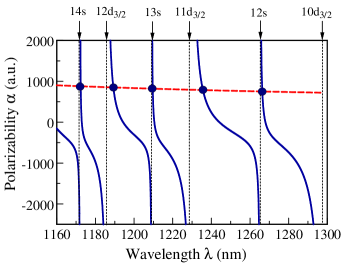
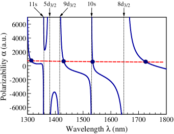
Figure 1: (Color online) The frequency-dependent polarizabilities of the Cs $6s$ and $7p_{1/2}$ states. The magic wavelengths are marked with circles. The approximate positions of the $7p_{1/2}-nl$ resonances are indicated by vertical lines with small arrows on top of the graph.

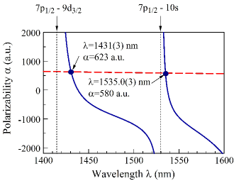
Figure 2: (Color online) The frequency-dependent polarizabilities of the Cs $6s$ and $7p_{1/2}$ states. The magic wavelengths are marked with circles and arrows. The approximate positions of the $7p_{1/2}-9d_{3/2}$ and $7p_{1/2}-10s$ resonances are indicated by vertical lines with small arrows on top of the graph.

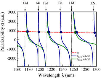
Figure 3: (Color online) The frequency-dependent polarizabilities of the Cs $6s$ and $7p_{3/2}$ states. The magic wavelengths are marked with circles. The approximate positions of the $7p_{3/2}-nl$ resonances are indicated by vertical lines with small arrows on top of the graph.

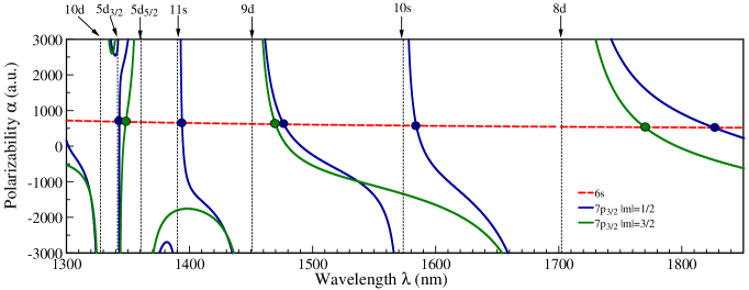
Figure 4: (Color online) The frequency-dependent polarizabilities of the Cs $6s$ and $7p_{3/2}$ states. The magic wavelengths are marked with circles and arrows. The approximate positions of the $7p_{3/2}-nl$ resonances are indicated by vertical lines with small arrows on top of the graph.

IV Static quadrupole polarizabilities of the $6s$ state

The static multipole polarizability $\alpha^{Ek}$ of Cs in its $6s$ state can be separated into two terms; a dominant first term from intermediate valence-excited states, and a smaller second term from the core-excited states. The second term is the lesser of these and is evaluated here in the random-phase approximation Johnson et al. (1983). The dominant valence contribution is calculated using the sum-over-state approach

$$\alpha^{Ek}_{v}=\frac{1}{2k+1}\sum_{n}\frac{|\langle nl_{j}\|r^{k}C_{kq}\|6s\rangle|^{2}}{E_{nlj}-E_{6s}},$$ (1)

where $C_{kq}(\hat{r})$ is a normalized spherical harmonic and where $nl$ is $np$, $nd$, and $nf$ for $k$ = 1, 2, and 3, respectively Johnson et al. (1995). Here we dicuss the the quadrupole ($k=2$) polarizabilities.

We use recommended energies from nis and our final quadrupole matrix elements to evaluate terms in the sum with $n\leq 13$, and we use theoretical SD energies and matrix elements to evaluate terms with $13\leq n\leq 26$. The remaining contributions to $\alpha^{E2}$ from orbitals with $27\leq n\leq 70$ are evaluated in the random-phase approximation (RPA). We find that this contribution is negligible. The uncertainties in the polarizability contributions are obtained from the uncertainties in the corresponding matrix elements. The final values for the quadrupole matrix elements and their uncertainties are determined using the same procedure as for the dipole matrix elements.

Contributions to the quadrupole polarizability of the $6s$ ground state are presented in Table 3. While the first two terms in the sum-over-states for the electric dipole polarizability contribute 99.5%, the first two terms in the sum-over-states for $\alpha^{E2}$ contribute 82.4%. The first eight terms gives 93.6%. The remaining 6.4% of $\alpha^{E2}$ contributions are from the $(9-26)nd$ states. Single-photon laser excitation of the $6s-5d$ transition has been used in Cs spectroscopy Weber and Sansonetti (1987), and the transition rate can be calculated from data in Table 3.

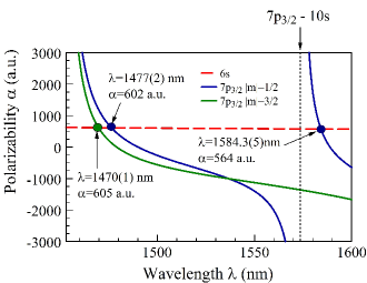
Figure 5: (Color online) The frequency-dependent polarizabilities of the Cs $6s$ and $7p_{3/2}$ states. The magic wavelengths are marked with circles and arrows. The approximate position of the and $7p_{3/2}-10s$ resonance is indicated by vertical line with small arrows on top of the graph.

V Scalar and tensor polarizabilities for excited states of cesium

The frequency-dependent scalar polarizability, $\alpha(\omega)$, of an alkali-metal atom in the state $v$ may be separated into a contribution from the ionic core, $\alpha_{\rm{core}}$, a core polarizability modification due to the valence electron, $\alpha_{vc}$, and a contribution from the valence electron, $\alpha^{v}(\omega)$. We find scalar Cs⁺ ionic core polarizability, calculated in random-phase approximation (RPA) to be 15.84 $a_{0}^{3}$, which is consistent with other data (see Table 4 of Ref. Mitroy et al. (2010)). A counter term $\alpha_{\rm vc}$ compensates for Pauli principle violating core-valence excitation from the core to the valence shell. It is small, $\alpha_{\rm vc}=-0.673$ a.u. for the $6s$ state of Cs. Since the core is isotropic, it makes no contribution to tensor polarizabilities.

The valence contribution to frequency-dependent scalar $\alpha_{0}$ and tensor $\alpha_{2}$ polarizabilities is evaluated as the sum over intermediate $k$ states allowed by the electric-dipole selection rules Mitroy et al. (2010)

$$\alpha_{0}^{v}(\omega) = \frac{2}{3(2j_{v}+1)}\sum_{k}\frac{{\left\langle k\left\|D\right\|v\right\rangle}^{2}(E_{k}-E_{v})}{(E_{k}-E_{v})^{2}-\omega^{2}},$$

$$\alpha_{2}^{v}(\omega) = -4C\sum_{k}(-1)^{j_{v}+j_{k}+1}\left\{\begin{array}[]{ccc}j_{v}&1&j_{k}\\ 1&j_{v}&2\\ \end{array}\right\}$$ (5)

$$\times\frac{{\left\langle k\left\|D\right\|v\right\rangle}^{2}(E_{k}-E_{v})}{(E_{k}-E_{v})^{2}-\omega^{2}},$$

where $C$ is given by

$$C=\left(\frac{5j_{v}(2j_{v}-1)}{6(j_{v}+1)(2j_{v}+1)(2j_{v}+3)}\right)^{1/2}$$

In the equations above, $\omega$ is assumed to be at least several linewidths off resonance with the corresponding transitions and ${\left\langle k\left\|D\right\|v\right\rangle}$ are the reduced electric-dipole matrix elements. Linear polarization is assumed in all calculation. To calculate static polarizabilities, we take $\omega=0$. The excited state polarizability calculations are carried out in the same way as the calculations of the multipole polarizabilities discussed in the previous section.

Contributions to the polarizabilities of the $6p_{1/2}$, $6p_{3/2}$ levels, $5d_{3/2}$ and $5d_{5/2}$ state of cesium are given in the Supplemental material SM . In Table 5, we list the $\alpha_{0}$ scalar and $\alpha_{2}$ tensor polarizabilities (in multiples of 1000 a.u.) in cesium. Uncertainties are given in parenthesis.

The largest (86.6%) contribution to the $\alpha_{0}(6p_{1/2})$ value arises from the the $6p_{1/2}-5d_{3/2}$ transition. The contribution of the $6s$ and $7s$ states in the $\alpha_{0}(6p_{1/2})$ value nearly cancel each other. Some cancellations are also observed in the breakdown of the $5d_{3/2}$ polarizability. We find that highly-excited $(9-26)f$ states contribute significantly, to the $5d_{3/2}$ and $5d_{5/2}$ polarizabilities, 14% and 11%, respectively.

We list the scalar polarizabilities of the $(7-13)s$, $(6-12)np$, and $(5-12)d$, and tensor polarizabilities of the $(6-12)np_{3/2}$ and $(5-12)d$ states in Table 4. Uncertainties are given in parenthesis. Comparison with theoretical results from van Wijngaarden and Li van Wijngaarden and Li (1994), Iskrenova-Tchoukova et al. Iskrenova-Tchoukova et al. (2007), and Mitroy et al. Mitroy et al. (2010) are given in the Supplemental Material SM . Results in the review paper Mitroy et al. (2010) are taken from paper Iskrenova-Tchoukova et al. (2007). The calculations of Ref. Iskrenova-Tchoukova et al. (2007) were also obtained using the single-double all-order method. In the present work, we treat higher-excited states more accurately, carrying all-order calculations up to $n=26$ instead of $n=12$. As we noted above, higher-excited states are particulary important for the $nd$ polarizabilities so the only significant differences with results of  Iskrenova-Tchoukova et al. (2007); Mitroy et al. (2010) occur for the $5d$ polarizabilities.

The scalar and tensor polarizabilities in van Wijngaarden and Li (1994) were evaluated using the Coulomb approximation. The expected scaling of polarizabilities as $(n^{*})^{7}$, where $n^{*}$ is the effective principal quantum number, was found to hold well for the higher excited states. Our values for the $n$ = 11 and 12 polarizabilities agree to 1% with van Wijngaarden and Li (1994).

Table 5: Magic wavelengths in nm for the $6s-7p$ transitions in Cs in the 1160-1800 nm wavelength range. The corresponding polarizabilities at magic wavelengths are given in a.u. The resonances near the magic wavelengths are listed in the first column.

Resonance	$\lambda_{\textrm{magic}}$	$\alpha(\lambda_{\textrm{magic}})$
$6s-7p_{1/2}$ transition
$7p_{1/2}-14s$	1172.40(3)	866
$7p_{1/2}-12d_{3/2}$	1189.3(4)	838
$7p_{1/2}-13s$	1209.68(4)	807
$7p_{1/2}-11d_{3/2}$	1235.7(5)	774
$7p_{1/2}-12s$	1266.4(1)	740
$7p_{1/2}-10d_{3/2}$	1313(6)	698
$7p_{1/2}-9d_{3/2}$	1431(3)	623
$7p_{1/2}-10s$	1535.0(3)	580
$7p_{1/2}-8d_{3/2}$	1727(5)	530
$6s-7p_{3/2}$, $|m|=1/2$ transition
$7p_{3/2}-13d_{3/2}$	1178.3(4)	856
$7p_{3/2}-14s$	1198.18(4)	824
$7p_{3/2}-12d_{3/2}$	1216.1(4)	799
$7p_{3/2}-13s$	1237.31(7)	772
$7p_{3/2}-11d_{3/2}$	1265.5(8)	741
$7p_{3/2}-12s$	1297.5(4)	711
$7p_{3/2}-5d_{3/2}$	11343(2)	675
$7p_{3/2}-11s$	1394.0(3)	643
$7p_{3/2}-9d_{3/2}$	1477(2)	602
$7p_{3/2}-10s$	1584.3(5)	564
$7p_{3/2}-8d_{3/2}$	1827(6)	512
$6s-7p_{3/2}$, $|m|=3/2$ transition
$7p_{3/2}-13d_{3/2}$	1177.5(4)	857
$7p_{3/2}-12d_{3/2}$	1215.0(4)	800
$7p_{3/2}-11d_{5/2}$	1263.3(5)	743
$7p_{3/2}-5d_{3/2}$	1348(4)	671
$7p_{3/2}-9d_{5/2}$	1470(1)	605
$7p_{3/2}-8d_{5/2}$	1770(3)	521

VI Magic wavelengths

Magic wavelengths for $D_{1}$ and $D_{2}$ lines in alkali-metal atoms were recently investigated in Refs. Arora et al. (2007); Flambaum et al. (2008); Derevianko (2010); Zhang et al. (2011). Flambaum et al. Flambaum et al. (2008) considered magic conditions for the ground state hyperfine clock transitions of cesium and rubidium atoms which used as the primary and the secondary frequency standards. The theory of magic optical traps for Zeeman-insensitive clock transitions in alkali-metal atoms was developed by Derevianko Derevianko (2010). Zhang et al. Zhang et al. (2011) proposed blue-detuned optical traps that were suitable for trapping of both ground-state and Rydberg excited atoms.

Several magic wavelengths were calculated for the $6s-6p_{1/2}$ and $6s-7p_{3/2}$ transitions in Cs in Ref. Arora et al. (2007) using the all-order approach. In this work, we present several other magic wavelengths for for the $6s-7p_{1/2}$ and $6s-7p_{3/2}$ transitions in Cs.

The magic wavelength $\lambda_{\rm{magic}}$ is defined as the wavelength for which the frequency-dependent polarizabilities of two atomic states are the same, leading to a vanishing ac Stark shift for that transition. To determine magic wavelengths for the $6s-7p$ transition, one calculates $\alpha_{6s}(\lambda)$ and $\alpha_{7p}(\lambda)$ polarizabilities and finds the wavelengths at which two respective curves intersect. All calculations are carried out for linear polarization.

The frequency-dependent polarizabilities are calculated the same way as the static polarizabilities, but setting $\omega\neq 0$. The dependence of the core polarizability on the frequency is negligible for the infrared frequencies of interests for this work. Therefore, we use the RPA static numbers for the ionic core and $\alpha_{vc}$ terms.

The total polarizability is given by

$$\alpha=\alpha_{0}+\alpha_{2}\frac{3m^{2}-j(j+1)}{j(2j-1)},$$

where $j$ is the total angular momentum and $m$ is corresponding magnetic quantum number. The total polarizability for the $7p_{3/2}$ states is given by

$$\alpha=\alpha_{0}-\alpha_{2}$$

for $m=\pm 1/2$ and

$$\alpha=\alpha_{0}+\alpha_{2}$$

for the $m=\pm 3/2$ case. Therefore, the total polarizability of the $7p_{3/2}$ state depends upon its $m$ quantum number and the magic wavelengths needs to be determined separately for the cases with $m=\pm 1/2$ and $m=\pm 3/2$ for the $6s-7p_{3/2}$ transitions, owing to the presence of the tensor contribution to the total polarizability of the $7p_{3/2}$ state. There is no tensor contribution to the polarizability of the $7p_{1/2}$ state. To determine the uncertainty in the values of magic wavelengths, we first determine the uncertainties in the polarizability values at the magic wavelengths. Then, the uncertainties in the values of magic wavelengths are determined as the maximum differences between the central value and the crossings of the $\alpha_{6s}\pm\delta\alpha_{6s}$ and $\alpha_{7p}\pm\delta\alpha_{7p}$ curves, where the $\delta\alpha$ are the uncertainties in the corresponding $6s$ and $7p$ polarizabilities.

Our magic wavelength results are given by Figs. 1, 2, 3, 4, 5, and Table 5. The frequency-dependent polarizabilities of the $6s$ and $7p_{1/2}$ states for $\lambda$ =1160 nm $-$ 1800 nm are plotted in Fig. 1. The magic wavelengths occur between the resonances corresponding to the $7s_{1/2}-nl$ transitions since the $6s$ polarizability curve has no resonances in this region and is nearly flat. Magic wavelengths are indicated by filled circles. The approximate positions of the $7s_{1/2}-nl$ resonances are indicated by the lines with small arrows on top of the graph, together with the corresponding $nl$ label. The $\lambda$ =1160 nm $-$ 1800 nm region contains resonances with $nl=5d,8d-12d$ and $nl=10s-14s$. Resonant wavelengths are listed in the last table of the Supplemental Material  SM . The $5d$ energy levels are below the $7p$ energy levels, while all of the other levels are above the $7p$, leading to interesting features of the $7p$ polarizability curves near the $7p-5d$ resonances. Due to particular experimental interest in the magic wavelength in the region nearly 1550 nm due to availability of the corresponding laser, we show more detailed plot of the frequency-dependent polarizabilities of the $6s$ and $7p_{1/2}$ states in the $\lambda$ = 1440 $-$ 1600 nm region in Fig. 2. The numerical values of these magic wavelengths are given in Table 5.

The frequency-dependent polarizabilities of the $6s$ and $7p_{3/2}$ states for $\lambda$ =1160 nm $-$ 1850 nm are plotted in Figs. 3 and 4. The numerical values of these magic wavelengths are given in Table 5. A detailed plot of the $\lambda$ = 1440 $-$ 1600 nm region is shown in Fig. 5. With the exception of the $7p_{3/2}-5d$ case, $7p_{3/2}-nd_{3/2}$ and $7p_{3/2}-nd_{5/2}$ resonances are too close together to show by separate lines on the plots due to small difference in the $nd_{3/2}$ and $nd_{5/2}$ energies for large $n$. Therefore, we indicate both $7p_{3/2}-nd_{3/2}$ and $7p_{3/2}-nd_{5/2}$ resonances by a single vertical line in Figs. 3, 4, and  5 with the “$nd$” label on the top. While there will be additional magic wavelengths in between the $7p_{3/2}-nd_{3/2}$ and $7p_{3/2}-nd_{5/2}$ resonances, we expect them to be unpractical to use in the experiment due to very strong dependence of polarizabilities on the wavelengths in these cases. Therefore, we omit such magic wavelengths in Table 5 and corresponding figures.

In summary, we carried out a systematic study of Cs atomic properties using all-order methods. Several calculations are carried out to evaluate uncertainties of the final results. Cs properties are needed for interpretation of the current experiments as well as planning of future experimental studies.

This research was performed under the sponsorship of the U.S. Department of Commerce, National Institute of Standards and Technology, and was supported by the National Science Foundation via the Physics Frontiers Center at the Joint Quantum Institute.

References

- Heavner et al. (2014) T. P. Heavner, E. A. Donley, F. Levi, G. Costanzo, T. E. Parker, J. H. Shirley, N. Ashby, S. Barlow, and S. R. Jefferts, Metrologia 51, 174 (2014).
- Jefferts et al. (2014) S. R. Jefferts, T. P. Heavner, T. E. Parker, J. H. Shirley, E. A. Donley, N. Ashby, F. Levi, D. Calonico, and G. A. Costanzo, Phys. Rev. Lett. 112, 050801 (2014).
- Porsev et al. (2009) S. G. Porsev, K. Beloy, and A. Derevianko, Phys. Rev. Lett. 102, 181601 (2009).
- Huntemann et al. (2014) N. Huntemann, B. Lipphardt, C. Tamm, V. Gerginov, S. Weyers, and E. Peik, Phys. Rev. Lett. 113, 210802 (2014).
- Clark et al. (2015) L. W. Clark, L.-C. Ha, C.-Y. Xu, and C. Chin, Phys. Rev. Lett. 115, 155301 (2015).
- Wang et al. (2015) Y. Wang, X. Zhang, T. A. Corcovilos, A. Kumar, and D. S. Weiss, Phys. Rev. Lett. 115, 043003 (2015).
- Tang et al. (2015) C. Tang, T. Zhang, and D. Weiss, in APS Division of Atomic, Molecular and Optical Physics Meeting Abstracts (2015).
- Hamilton et al. (2015) P. Hamilton, M. Jaffe, J. M. Brown, L. Maisenbacher, B. Estey, and H. Müller, Phys. Rev. Lett. 114, 100405 (2015).
- Patton et al. (2014) B. Patton, E. Zhivun, D. C. Hovde, and D. Budker, Phys. Rev. Lett. 113, 013001 (2014).
- Wolf et al. (2006) P. Wolf, F. Chapelet, S. Bize, and A. Clairon, Phys. Rev. Lett. 96, 060801 (2006).
- Mitroy et al. (2010) J. Mitroy, M. S. Safronova, and C. W. Clark, J. Phys. B 43, 202001 (2010).
- Katori et al. (1999) H. Katori, T. Ido, and M. Kuwata-Gonokami, J. Phys. Soc. Jpn. 668, 2479 (1999).
- Ye et al. (1999) J. Ye, D. W. Vernooy, and H. J. Kimble, Phys. Rev. Lett. 83, 4987 (1999).
- Duarte et al. (2011) P. M. Duarte, R. A. Hart, J. M. Hitchcock, T. A. Corcovilos, T.-L. Yang, A. Reed, and R. G. Hulet, Phys. Rev. A 84, 061406R (2011).
- McKay et al. (2011) D. C. McKay, D. Jervis, D. J. Fine, J. W. Simpson-Porco, G. J. A. Edge, and J. H. Thywissen, Phys. Rev. A 84, 063420 (2011).
- Safronova and Johnson (2008) M. S. Safronova and W. R. Johnson, Adv. At. Mol. Opt. Phys. 55, 191 (2008).
- Robyr et al. (2014) J.-L. Robyr, P. Knowles, and A. Weis, Phys. Rev. A 90, 012505 (2014).
- Antypas and Elliott (2011) D. Antypas and D. S. Elliott, Phys. Rev. A 83, 062511 (2011).
- Kortyna et al. (2011) A. Kortyna, C. Tinsman, J. Grab, M. S. Safronova, and U. I. Safronova, Phys. Rev. A 83, 042511 (2011).
- Zhao et al. (2011) J.-M. Zhao, H. Zhang, Z.-G. Feng, X.-B. Zhu, L.-J. Zhang, C.-Y. Li, and S.-T. Jia, J. Phys. Soc. Jpn. 80, 034303 (2011).
- Auzinsh et al. (2007) M. Auzinsh, K. Bluss, R. Ferber, F. Gahbauer, A. Jarmola, M. S. Safronova, U. I. Safronova, and M. Tamanis, Phys. Rev. A 75, 022502 (2007).
- Ulzega et al. (2007) S. Ulzega, A. Hofer, P. Moroshkin, R. Müller-Siebert, D. Nettels, and A. Weis, Phys. Rev. A 75, 042505 (2007).
- Gunawardena et al. (2007) M. Gunawardena, D. S. Elliott, M. S. Safronova, and U. Safronova, Phys. Rev. A 75, 022507 (2007).
- Sieradzan et al. (2004) A. Sieradzan, M. D. Havey, and M. S. Safronova, Phys. Rev. A 69, 022502 (2004).
- Amini and Gould (2003) J. M. Amini and H. Gould, Phys. Rev. Lett. 91, 153001 (2003).
- Ospelkaus et al. (2003) C. Ospelkaus, U. Rasbach, and A. Weis, Phys. Rev. A 67, 011402 (2003).
- Bennett and Wieman (1999) S. C. Bennett and C. E. Wieman, Phys. Rev. Lett. 82, 2484 (1999).
- Yei et al. (1998) W. Yei, A. Sieradzan, E. Cerasuolo, and M. D. Havey, Phys. Rev. A 57, 3419 (1998).
- Cho et al. (1997) D. Cho, C. S. Wood, S. C. Bennett, J. L. Roberts, and C. E. Wieman, Phys. Rev. A 55, 1007 (1997).
- Kamenski and Ovsiannikov (2014) A. A. Kamenski and V. D. Ovsiannikov, J. Phys. B 47, 095002 (2014).
- Tang et al. (2014) Y.-B. Tang, C.-B. Li, and H.-X. Qiao, Chin. Phys. B 23, 063101 (2014).
- Roberts et al. (2013) B. M. Roberts, V. A. Dzuba, and V. V. Flambaum, Phys. Rev. A 88, 042507 (2013).
- Derevianko et al. (2010) A. Derevianko, S. G. Porsev, and J. F. Babb, At. Data Nucl. Data Tables 96, 323 (2010).
- Dzuba et al. (2010) V. A. Dzuba, V. V. Flambaum, K. Beloy, and A. Derevianko, Phys. Rev. A 82, 062513 (2010).
- Kondratjev et al. (2010) D. A. Kondratjev, I. L. Beigman, and L. A. Vainshtein, J. Russ. Laser Res. 31, 294 (2010).
- Il’inova et al. (2009) E. Y. Il’inova, A. A. Kamenski, and V. D. Ovsiannikov, J. Phys. B 42, 145004 (2009).
- Hofer et al. (2008) A. Hofer, P. Moroshkin, S. Ulzega, and A. Weis, Phys. Rev. A 77, 012502 (2008).
- Iskrenova-Tchoukova et al. (2007) E. Iskrenova-Tchoukova, M. S. Safronova, and U. I. Safronova, J. Comput. Methods Sciences and Eng. 7, 521 (2007).
- Ulzega et al. (2006) S. Ulzega, A. Hofer, P. Moroshkin, and A. Weis, Europhys. Lett. 76, 1074 (2006).
- Porsev and Derevianko (2006) S. G. Porsev and A. Derevianko, Phys. Rev. A 74, 020502 (2006).
- Safronova et al. (2006) M. S. Safronova, B. Arora, and C. W. Clark, Phys. Rev. A 73, 022505 (2006).
- Lim et al. (2005) I. S. Lim, P. Schwerdtfeger, B. Metz, and H. Stoll, J. Chem. Phys. 122, 104103 (2005).
- Safronova and Clark (2004) M. S. Safronova and C. W. Clark, Phys. Rev. A 69, 040501 (2004).
- Magnier and Aubert-Frécon (2002) S. Magnier and M. Aubert-Frécon, J. Quant. Spectrosc. Radiat. Transfer 75, 121 (2002).
- Safronova et al. (1999) M. S. Safronova, W. R. Johnson, and A. Derevianko, Phys. Rev. A 60, 4476 (1999).
- Lim et al. (1999) I. S. Lim, M. Pernpointner, M. Seth, J. K. Laerdahl, P. Schwerdtfeger, P. Neogrady, and M. Urban, Phys. Rev. A 60, 2822 (1999).
- Xia et al. (1997) J. Xia, J. Clarke, J. Li, and W. A. van Wijngaarden, Phys. Rev. A 56, 5176 (1997).
- van Wijngaarden and Li (1994) W. A. van Wijngaarden and J. Li, J. Quant. Spectrosc. Radiat. Transfer 52, 555 (1994).
- Fuentealba and Reyes (1993) P. Fuentealba and O. Reyes, J. Phys. B 26, 2245 (1993).
- Johnon et al. (1996) W. R. Johnon, Z. W. Liu, and J. Sapirstein, At. Data and Nucl. Data Tables 64, 279 (1996).
- (51) See Supplemental Material at URL for additional Cs data.
- (52) Kramida, A., Ralchenko, Yu., Reader, J., and NIST ASD Team (2014). NIST Atomic Spectra Datab ase (ver. 5.2), [Online]. Available: http://physics.nist.gov/asd [2015, September 3]. National Institute of Standards and Technology, Gaithersburg, MD.
- Safronova and Safronova (2011) U. I. Safronova and M. S. Safronova, Canadian Journal of Physics 89, 465 (2011).
- Safronova and Safronova (2014) U. I. Safronova and M. S. Safronova, Phys. Rev. A 89, 052515 (2014).
- Young et al. (1994) L. Young, W. T. H. III, S. J. Sibener, S. D. Price, C. E. Tanner, C. E. Wieman, and S. R. Leone, Phys. Rev. A 50, 2174 (1994).
- Sell et al. (2011) J. F. Sell, B. M. Patterson, T. Ehrenreich, G. Brooke, J. Scoville, and R. J. Knize, Phys. Rev. A 84, 010501 (2011).
- DiBerardino et al. (1998) D. DiBerardino, C. E. Tanner, and A. Sieradzan, Phys. Rev. A 57, 4204 (1998).
- Marek (1977a) J. Marek, J. Phys. B 10, p. L325 (1977a).
- Ortiz and Campos (1981) M. Ortiz and J. Campos, J. Quant. Spectrosc. Radiat. Transfer 26, 107 (1981).
- Marek and Ryschka (1979) J. Marek and M. Ryschka, Phys. Lett. A 74, 51 (1979).
- Marek (1977b) J. Marek, Phys. Lett. A 60, 190 (1977b).
- Marek and Niemax (1976) J. Marek and K. Niemax, J. Phys. B 9, p. L483 (1976).
- Neil and Atkinson (1984) W. S. Neil and J. B. Atkinson, J. Phys. B 17, 693 (1984).
- Sieradzan et al. (1979) A. Sieradzan, W. Jastrzebski, and J. Krasinski, Opt. Commun. 28, 73 (1979).
- Safronova and Safronova (2011) M. S. Safronova and U. I. Safronova, Phys. Rev. A 83, 052508 (2011).
- Safronova and Safronova (2012) M. S. Safronova and U. I. Safronova, Phys. Rev. A 85, 022504 (2012).
- Gallagher (1967) A. Gallagher, Phys. Rev. 157, 68 (1967).
- Schmieder and Lurio (1970) R. W. Schmieder and A. Lurio, Phys. Rev. A 2, 1216 (1970).
- Bulos et al. (1976) B. R. Bulos, R. Gupta, and W. Happer, J. Opt. Soc. Am. 66, 426 (1976).
- Deech et al. (1977) J. S. Deech, R. Luypaert, L. R. Pendrill, and G. W. Series, J. Phys. B 10, p. L137 (1977).
- Alessandretti et al. (1977) G. Alessandretti, F. Chiarini, G. Gorini, and F. Petrucci, Opt. Commun. 20, 289 (1977).
- Bouchiat et al. (1992) M. A. Bouchiat, J. Guéna, P. Jacquier, and M. Lintz, Z. Phys. D 24, 335 (1992).
- Hoeling et al. (1996) B. Hoeling, J. R. Yeh, T. Takekoshi, and R. J. Knize, Opt. Lett. 21, 74 (1996).
- Tanner et al. (1992) C. E. Tanner, A. E. Livingston, R. J. Rafac, F. G. Serpa, K. W. Kukla, H. G. Berry, L. Young, and C. A. Kurtz, Phys. Rev. Lett. 69, 2765 (1992).
- Rafac et al. (1994) R. J. Rafac, C. E. Tanner, A. E. Livingston, K. W. Kukla, H. G. Berry, and C. A. Kurtz, Phys. Rev. A 50, p. R1976 (1994).
- Rafac et al. (1999) R. J. Rafac, C. E. Tanner, A. E. Livingston, and H. G. Berry, Phys. Rev. A 60, 3648 (1999).
- Johnson et al. (1983) W. R. Johnson, D. Kolb, and K.-N. Huang, At. Data Nucl. Data Tables 28, 333 (1983).
- Johnson et al. (1995) W. R. Johnson, D. R. Plante, and J. Sapirstein, Adv. Atom. Mol. Opt. Phys. 35, 255 (1995).
- Weber and Sansonetti (1987) K.-H. Weber and C. J. Sansonetti, Phys. Rev. A 35, 4650 (1987), URL http://link.aps.org/doi/10.1103/PhysRevA.35.4650.
- Arora et al. (2007) B. Arora, M. S. Safronova, and C. W. Clark, Phys. Rev. A 76, 052509 (2007).
- Flambaum et al. (2008) V. V. Flambaum, V. A. Dzuba, and A. Derevianko, Phys. Rev. Lett. 101, 220801 (2008).
- Derevianko (2010) A. Derevianko, Phys. Rev. A 81, 051606 (2010).
- Zhang et al. (2011) S. Zhang, F. Robicheaux, and M. Saffman, Phys. Rev. A 84, 043408 (2011).