Electrical and optical conductivities of hole gas in $p$-doped bulk III-V semiconductors

Abstract

We study electrical and optical conductivities of hole gas in $p$-doped bulk III-V semiconductors described by the Luttinger Hamiltonian. We provide exact analytical expressions of the Drude conductivity, inverse relaxation time for various impurity potentials, Drude weight and optical conductivity in terms of the Luttinger parameters $\gamma_{1}$ and $\gamma_{2}$. The back scattering is completely suppressed as a result of the helicity conservation of the heavy and light hole states. The energy dependence of the relaxation time for the hole states is different from the Brooks-Herring formula for electron gas in $n$-doped semiconductors. We find that the inverse relaxation time of heavy holes is much less than that of the light holes for Coulomb-type and Gaussian-type impurity potentials and vice-versa for short-range impurity potential. The Drude conductivity increases non-linearly with the increase of the hole density. The exponent of the density dependence of the conductivity is obtained in the Thomas-Fermi limit. The Drude weight varies linearly with the density even in presence of the spin-orbit coupling. The finite-frequency optical conductivity goes as $\sqrt{\omega}$ and its amplitude strongly depends on the Luttinger parameters. The Luttinger parameters can be extracted from the optical conductivity measurement.

I Introduction

There is a renewed research interest on various properties of $p$-doped zinc-blende semiconductors described by the Luttinger Hamiltonian Lutin for the spin-3/2 valence band, after the theoretical proposal of intrinsic SHE put forward by Murakami et al. murakami1 . The intrinsic SHE is solely due to the presence of the spin-orbit coupling in the bands even in absence of any impurities. Later, this exotic phenomena has been observed experimentally in bulk n-doped semiconductors such as GaAs and InGaAs she-exp as well as in two-dimensional hole gas she-exp1 .

A large number of theoretical studies have been carried out on $p$-doped bulk III-V semiconductors in recent years. Quantum mechanical calculations of spin Hall conductivity by defining the exact conserved spin current of $p$-doped bulk semiconductors describing by the Luttinger Hamiltonian is provided in Ref. murakami2 . The wave packet dynamics in the bulk $p$-doped hole gas has been studied in details zb1 ; zb2 ; zb3 . A theoretical study of interacting hole gas in $p$-doped bulk III-V semiconductors has been done using the self-consistent Hartree-Fock methodjSc1 . The dielectric function and beating pattern of the Friedel oscillations of the bulk hole liquid within the random phase approximation are also studied jSc2 ; jSc3 . There have been extensive theoretical fms-t ; fms-t1 and experimental fms-e ; fms-e1 ; fms-e2 ; fms-e3 ; fms-e4 studies on $p$-doped III-V ferromagnetic semiconductors fms-rev such as GaMnAs and InMnAs with the Curie temperature T<170 K. Recently, the magnetotransport coefficients of the Luttinger Hamiltonian have been studied numerically sdh .

Studies of the electrical conductivity helps to determine the nature of the interaction between charge carriers and impurities. On the other hand, the optical transitions between spin-split Fermi surfaces provide the information about the curvature of the complex energy bands. To the best of our knowledge, DC and AC electric fields response to the 3D hole gas in $p$-doped bulk semiconductors are lacking. The nature of the complex valence bands and values of the Luttinger parameters can be extracted from the electrical and optical conductivities. Therefore, theoretical studies of the electrical and optical conductivities would help to analyze the experimental observations. Theoretical studies of the Drude and optical conductivities of two-dimensional hole gas with $k$-cubic Rashba and Dresselhaus spin-orbit interactions are given in Refs. opt4 ; opt5 .

In this work, we consider hole gas in $p$-doped bulk III-V semiconductors described by the Luttinger Hamiltonian subjected to static and time-varying electric fields and study Drude conductivity, inverse relaxation time, Drude weight and optical conductivity. The exact analytical expressions of the Drude conductivity, inverse relaxation times for various impurity potentials, the Drude weight and optical conductivity are provided. We show that the back scattering is completely suppressed due to the helicity conservation of the heavy and light hole states. The zero-frequency Drude weight is linear with respect to the carrier density even in the presence of the spin-orbit coupling, due to $k^{2}$-dependence of the spin-orbit interaction. A minimum photon energy is required to trigger the optical transition and then the optical conductivity grows as $\sqrt{\omega}$ ($\hbar\omega$ is the photon energy) and cease to zero beyond some critical photon energy depending on the Luttinger parameters and hole density. We show that the Luttinger parameters can be extracted from the optical conductivity measurement.

This paper is organized as follows. The basic information of the physical system is described in section II. In section III, we present detail calculations of the Drude conductivity and the inverse relaxation time. In section IV, we present results of the Drude weight and the optical conductivity. An alternate derivation of the optical conductivity is provided in Appendix. The summary of this paper is presented in section V.

II Basic informations

The valence bands of common semiconductors having diamond and zinc-blende crystal structures can be accurately described by the following $6\times 6$ Luttinger Hamiltonian Lutin6x6 :

$$H=\begin{bmatrix}-P-Q&L&-M&0&\frac{1}{\sqrt{2}}L&-\sqrt{2}M\\ L^{\dagger}&-P+Q&0&-M&\sqrt{2}Q&-\sqrt{\frac{3}{2}}L\\ -M^{\dagger}&0&-P+Q&-L&-\sqrt{\frac{3}{2}}L^{\dagger}&-\sqrt{2}Q\\ 0&-M^{\dagger}&-L^{\dagger}&-P-Q&\sqrt{2}M^{\dagger}&\frac{1}{\sqrt{2}}L^{\dagger}\\ \frac{1}{\sqrt{2}}L^{\dagger}&\sqrt{2}Q^{\dagger}&-\sqrt{\frac{3}{2}}L&\sqrt{2}M&-P-\Delta_{\rm so}&0\\ -\sqrt{2}M^{\dagger}&-\sqrt{\frac{3}{2}}L^{\dagger}&-\sqrt{2}Q^{\dagger}&\frac{1}{\sqrt{2}}L&0&-P-\Delta_{\rm so}\end{bmatrix},$$ (1)

where $P=\frac{\gamma_{1}\hbar^{2}}{2m_{0}}(k_{x}^{2}+k_{y}^{2}+k_{z}^{2}),Q=\frac{\gamma_{2}\hbar^{2}}{2m_{0}}(k_{x}^{2}+k_{y}^{2}-2k_{z}^{2}),L=\frac{\sqrt{3}\gamma_{3}\hbar^{2}}{m_{0}}(k_{x}-ik_{y})k_{z}$ and $M=-\frac{\sqrt{3}\hbar^{2}}{2m_{0}}[\gamma_{2}(k_{x}^{2}-k_{y}^{2})-2i\gamma_{3}k_{x}k_{y}]$. Here $m_{0}$ is the bare electron mass and $\Delta_{\rm so}$ being the split-off energy. Also, $\gamma_{1}$, $\gamma_{2}$ and $\gamma_{3}$ are the dimensionless Luttinger parameters characterizing the valence band of the specific semiconductors. The parameters $\gamma_{2}$ and $\gamma_{3}$ contain the information about the spin-orbit coupling. The Luttinger parameters $\gamma_{1}$, $\gamma_{2}$ and $\gamma_{3}$ along with other parameters of the band structure of various semiconductors are readily available in Ref. parameters . The Luttinger parameters in zinc-blende semiconductors are of the order of the same magnitude. It implies that the spin-orbit coupling is strong in bulk hole systems, in comparison to the bulk electron systems.

The split-off energy $\Delta_{\rm so}$ for these semiconductors is of the order of few hundred meV. On the other hand, the Fermi energy is of the order of few meV for typical hole density ($n_{h}\sim 10^{23}$ m${}^{-3})$. Thus, one can safely ignore the split-off band when the Fermi energy is sufficiently smaller than the split-off energy and hence the upper-left $4\times 4$ matrix block in Eq. (1) describes the two upper most valence bands (known as heavy hole and light hole bands) approximately. Within the spherical approximation ($\gamma_{3}=\gamma_{2}$), the 4 $\times$ 4 Luttinger’s Hamiltonian Lutin can be written in a compact form as

$$H=\frac{1}{2m_{0}}\Bigg{[}\Bigg{(}\gamma_{1}+\frac{5}{2}\gamma_{2}\Bigg{)}{\bf p}^{2}-2\gamma_{2}\big{(}{\bf p}\cdot{\bf S}\big{)}^{2}\Bigg{]}.$$ (2)

Here ${\bf p}$ is the hole momentum operator, ${\bf S}$ are the spin-3/2 operators arises from the addition of $l=1$ orbital angular momentum and $s=1/2$ spin angular momentum.

The spin-3/2 operators are given as

$$S_{x}=\begin{pmatrix}0&\frac{\sqrt{3}}{2}&0&0\\ \frac{\sqrt{3}}{2}&0&1&0\\ 0&1&0&\frac{\sqrt{3}}{2}\\ 0&0&\frac{\sqrt{3}}{2}&0\end{pmatrix},$$ (3)

$$S_{y}=i\begin{pmatrix}0&-\frac{\sqrt{3}}{2}&0&0\\ \frac{\sqrt{3}}{2}&0&-1&0\\ 0&1&0&-\frac{\sqrt{3}}{2}\\ 0&0&\frac{\sqrt{3}}{2}&0\end{pmatrix},$$ (4)

$$S_{z}=\begin{pmatrix}\frac{3}{2}&0&0&0\\ 0&\frac{1}{2}&0&0\\ 0&0&-\frac{1}{2}&0\\ 0&0&0&-\frac{3}{2}\end{pmatrix}.$$ (5)

The rotationally invariant Hamiltonian $H$ commutes with the helicity operator $\hat{\lambda}={\bf k}\cdot{\bf S}/k$ so that its eigenvalues $\lambda=\pm 3/2,\pm 1/2$ are good quantum numbers. Here $\lambda=\pm 3/2$ and $\lambda=\pm 1/2$ correspond to the heavy hole and light hole states, respectively. Therefore, the eigenstates of the helicity operator can be chosen as the eigenstates of the above Hamiltonian. The dispersion relations of the heavy and light hole states are given by

$$E_{h/l}({\bf k})=\frac{(\hbar k)^{2}}{2m_{h/l}}.$$ (6)

Here the heavy and light hole masses are $m_{h/l}=m_{0}/(\gamma_{1}\mp 2\gamma_{2})$, respectively. The two-fold degeneracy of heavy and light hole branches is due to the consequence of the space inversion and time-reversal symmetries of the Luttinger Hamiltonian. The corresponding eigenstates are given by

$$\psi_{\lambda,{\bf k}}({\bf r})=\frac{e^{i{\bf k\cdot r}}}{\sqrt{V}}|\phi_{\lambda}({\bf k})\rangle,$$ (7)

where $V$ is the volume of the system. Using the basis of eigenstates of $S_{z}$ and parameterizing ${\bf k}$ in terms of spherical polar coordinates as ${\bf k}=k(\sin\theta\cos\phi,\sin\theta\sin\phi,\cos\theta)$, the eigenspinors $|\phi_{\lambda}({\bf k})\rangle$ for $\lambda=3/2$ and $\lambda=1/2$ can be written as

$$|\phi_{3/2}({\bf k})\rangle=\begin{pmatrix}\cos^{3}\frac{\theta}{2}e^{(-3i/2)\phi}\\ \sqrt{3}\cos^{2}\frac{\theta}{2}\sin\frac{\theta}{2}e^{(-i/2)\phi}\\ \sqrt{3}\cos\frac{\theta}{2}\sin^{2}\frac{\theta}{2}e^{(i/2)\phi}\\ \sin^{3}\frac{\theta}{2}e^{(3i/2)\phi}\end{pmatrix}$$ (8)

and

$$|\phi_{1/2}({\bf k})\rangle=\begin{pmatrix}-\sqrt{3}\cos^{2}\frac{\theta}{2}\sin\frac{\theta}{2}e^{(-3i/2)\phi}\\ \cos\frac{\theta}{2}\Big{(}\cos^{2}\frac{\theta}{2}-2\sin^{2}\frac{\theta}{2}\Big{)}e^{(-i/2)\phi}\\ \sin\frac{\theta}{2}\Big{(}2\cos^{2}\frac{\theta}{2}-\sin^{2}\frac{\theta}{2}\Big{)}e^{(i/2)\phi}\\ \sqrt{3}\cos\frac{\theta}{2}\sin^{2}\frac{\theta}{2}e^{(3i/2)\phi}\end{pmatrix}.$$ (9)

The remaining spinors for $\lambda=-3/2$ and $\lambda=-1/2$ can easily be obtained from Eq. (8) and Eq. (9) under the spatial inversion operations $\theta\rightarrow\pi-\theta$ and $\phi\rightarrow\pi+\phi$.

In order to study transport properties and electrical/optical conductivities, we need to know the ground state properties such as the Fermi energy and the corresponding Fermi wave vectors of the two branches for a given hole density $n_{h}$. Following the standard procedure, the Fermi energy and the corresponding Fermi wave vector are respectively given by

$$E_{\rm f}=\frac{(\hbar{k_{\rm f}^{0}})^{2}}{2m_{0}}\bigg{[}\frac{\gamma_{1}^{2}-4\gamma_{2}^{2}}{\big{[}(\gamma_{1}-2\gamma_{2})^{3/2}+(\gamma_{1}+2\gamma_{2})^{3/2}\big{]}^{2/3}}\bigg{]}$$ (10)

and

$$k_{\rm f}^{h/l}=k_{\rm f}^{0}\frac{\sqrt{\gamma_{1}\pm 2\gamma_{2}}}{\big{[}(\gamma_{1}-2\gamma_{2})^{3/2}+(\gamma_{1}+2\gamma_{2})^{3/2}\big{]}^{1/3}},$$ (11)

where $k_{\rm f}^{0}=(3\pi^{2}n_{h})^{1/3}$. One can easily check that $E_{\rm f}\approx 2E_{\rm f}^{0}=(\hbar k_{f}^{0})^{2}/m_{0}$ for typical values of the Luttinger parameters.

The $x$, $y$ and $z$ components of the velocity operator (which will be required to calculate the Drude and optical conductivities) are as follows

$$\hat{v}_{x}({\bf k})=\begin{pmatrix}(\mathbb{I}\gamma_{1}+\gamma_{2}\sigma_{z})k_{x}-\sqrt{3}\gamma_{2}\sigma_{x}k_{z}&-\sqrt{3}\mathbb{I}\gamma_{2}k_{-}\\ -\sqrt{3}\mathbb{I}\gamma_{2}k_{+}&(\mathbb{I}\gamma_{1}-\gamma_{2}\sigma_{z})k_{x}+\sqrt{3}\gamma_{2}\sigma_{x}k_{z}\end{pmatrix},$$ (12)

$$\hat{v}_{y}({\bf k})=\begin{pmatrix}(\mathbb{I}\gamma_{1}+\gamma_{2}\sigma_{z})k_{y}-\sqrt{3}\gamma_{2}\sigma_{y}k_{z}&i\sqrt{3}\mathbb{I}\gamma_{2}k_{-}\\ -i\sqrt{3}\mathbb{I}\gamma_{2}k_{+}&(\mathbb{I}\gamma_{1}-\gamma_{2}\sigma_{z})k_{y}+\sqrt{3}\gamma_{2}\sigma_{y}k_{z}\end{pmatrix}$$ (13)

and

$$\hat{v}_{z}({\bf k})=\begin{pmatrix}(\mathbb{I}\gamma_{1}-\gamma_{2}\sigma_{z})k_{z}-\sqrt{3}\gamma_{2}(k_{x}\sigma_{x}+k_{y}\sigma_{y})&\mathbb{O}\\ \mathbb{O}&(\mathbb{I}\gamma_{1}+\gamma_{2}\sigma_{z})k_{z}+\sqrt{3}\gamma_{2}(k_{x}\sigma_{x}+k_{y}\sigma_{y})\end{pmatrix}.$$ (14)

Here $\mathbb{I}$ is a $2\times 2$ identity matrix, $\sigma_{x,y,z}$ are the Pauli’s $2\times 2$ matrices and $\mathbb{O}$ represents a $2\times 2$ null matrix.

III Drude Conductivity and Inverse relaxation time

III.1 Drude conductivity

With the application of weak DC electric field along $x$-direction ${\bf E}=E_{x}\hat{x}$, the hole current density is $J_{h}=\sigma_{xx}E_{x}$ with $\sigma_{xx}$ being the Drude conductivity. Within the semi-classical Boltzmann theory and the relaxation time approximation, the general expression of the Drude conductivity at very low temperature is given by mermin

$$\sigma_{xx}=\frac{e^{2}}{(2\pi)^{3}}\sum_{\lambda}\int d^{3}k\langle\hat{v}_{x}({\bf k})\rangle^{2}_{{}_{\lambda}}\,\tau_{\lambda}({\bf k})\,\delta[E_{\lambda}({\bf k})-E_{\rm f}],$$ (15)

where $\hat{v}_{x}({\bf k})$ is the $x$-component of the velocity operator and $\tau_{\lambda}({\bf k})$ is the relaxation time.

The expectation values of the velocity operator $\hat{v}_{x}$ with respect to the heavy hole and light hole states are $\langle\hat{v}_{x}({\bf k})\rangle_{h}=\hbar k_{x}/m_{h}$ and $\langle\hat{v}_{x}({\bf k})\rangle_{l}=\hbar k_{x}/m_{l}$. Using these results, the final expression of the Drude conductivity is obtained as

$$\sigma_{xx}=\frac{n_{h}e^{2}}{m_{0}}\bigg{[}\frac{\tau_{h}\sqrt{\gamma_{1}+2\gamma_{2}}+\tau_{l}\sqrt{\gamma_{1}-2\gamma_{2}}}{(\gamma_{1}-2\gamma_{2})^{3/2}+(\gamma_{1}+2\gamma_{2})^{3/2}}\bigg{]}(\gamma_{1}^{2}-4\gamma_{2}^{2}).$$ (16)

Here $\tau_{h}\equiv\tau_{h}(E_{\rm f})$ and $\tau_{l}\equiv\tau_{l}(E_{\rm f})$. Now we need to calculate relaxation time $\tau_{h}$ and $\tau_{l}$, which will be shown in the next section. In absence of the atomic spin-orbit coupling (i.e. $\gamma_{2}=0$), the Drude conductivity reduces to the known result. The Drude conductivity varies non-linearly with the Luttinger’s parameters due to the presence of the spin-orbit coupling $\gamma_{2}$.

III.2 Inverse relaxation time

In this section, we derive the expression of the inverse relaxation time for heavy hole and light hole bands. Within the semi-classical Boltzmann theory, the most general expression of the inverse relaxation time for a given band is given asmermin ,

$$\frac{1}{\tau_{\lambda}(k)}=V\int\frac{d^{3}k^{\prime}}{(2\pi)^{3}}W_{{\bf k}{\bf k}^{\prime}}^{\lambda}(1-\cos\theta^{\prime}),$$ (17)

where $\theta^{\prime}$ is the angle between the vectors ${\bf k}$ and ${\bf k}^{\prime}$ and the intra-band transition rate between the states $|{\bf k},\lambda\rangle$ and $|{\bf k^{\prime}},\lambda\rangle$ is

$$W_{{\bf k}{\bf k}^{\prime}}^{\lambda}=\frac{2\pi}{\hbar}N_{\textrm{\rm imp}}\big{|}\big{\langle}{\bf k^{\prime},\lambda}\big{|}V_{\textrm{imp}}^{\lambda}({\bf r})\big{|}{\bf k,\lambda}\rangle\big{|}^{2}\delta(E_{\lambda}({\bf k})-E_{\lambda}({\bf k^{\prime}})).$$

Here, $N_{\textrm{\rm imp}}$ is the number of impurities present in the system and $V_{\textrm{imp}}^{\lambda}({\bf r})$ is the impurity potential. The matrix element $\langle{\bf k^{\prime}},\lambda\big{|}V_{\textrm{imp}}^{\lambda}({\bf r})\big{|}{\bf k},\lambda\rangle$ is given by $\langle{\bf k}^{\prime},\lambda\big{|}V_{\textrm{imp}}^{\lambda}({\bf r})\big{|}{\bf k},\lambda\rangle=V_{\rm imp}^{\lambda}({\bf q})\phi_{\lambda}^{\dagger}({\bf k}^{\prime})\phi_{\lambda}({\bf k})/V,$ where $q=|{\bf k}-{\bf k}^{\prime}|$ being the change in the wave vector and $V_{\rm imp}^{\lambda}({\bf q})$ is the Fourier transform of the impurity potential $V_{\rm imp}^{\lambda}({\bf r})$. Therefore, the transition rate is given by

$$W_{{\bf k}{\bf k}^{\prime}}^{\lambda}=\frac{2\pi n_{\textrm{imp}}}{\hbar\,V}\big{|}V_{\rm imp}^{\lambda}({\bf q})\big{|}^{2}\big{|}\phi_{\lambda}^{\dagger}({\bf k}^{\prime})\phi_{\lambda}({\bf k})\big{|}^{2}\delta(E_{\lambda}({\bf k})-E_{\lambda}({\bf k^{\prime}}).$$

Here, $n_{\rm imp}=N_{\rm imp}/V$ is the impurity density and the square of the wave function overlaps are given by

$$|\phi_{h}^{\dagger}({\bf k^{\prime}})\phi_{h}({\bf k})|^{2}=\frac{(1+\cos\theta^{\prime})^{3}}{8}$$

and

$$|\phi_{l}^{\dagger}({\bf k^{\prime}})\phi_{l}({\bf k})|^{2}=\frac{(1+\cos\theta^{\prime})(3\cos\theta^{\prime}-1)^{2}}{8}.$$

It is interesting to note that the square of the wave function overlaps exactly vanish at $\theta^{\prime}=\pi$ and do not contribute to the scattering rates. It implies that the backscattering is completely suppressed. This can easily be understood from the helicity conservation. Since the helicity is a conserved quantity, the charge carriers can not change its momentum after scattering. This is similar to the absence of backscattering in monolayer graphene as a result of the pseudospin conservation ando ; ando1 . Moreover, the light hole scattering rate ($1/\tau_{l}$) is also suppressed at $\theta^{\prime}=\cos^{-1}(1/3)$. It should be mention here that the suppression of scattering in certain directions is independent of choice of the impurity potential.

We shall consider two long-range and one short-range impurity potentials to calculate $1/\tau_{\lambda}$ and $\sigma_{xx}$.
i) Coulomb impurity potential: First we consider screened Coulomb-type impurity potential, $V_{\rm imp}^{\lambda}({\bf r})=[Ze^{2}/(4\pi\epsilon)]\mathrm{e}^{-k_{s}^{\lambda}r}/r$, where $\epsilon$ is the static dielectric constant and $k_{s}^{\lambda}$ is the Thomas-Fermi screening wave-vector, given by ${k_{s}^{\lambda}}=\sqrt{4k_{\rm f}^{\lambda}/(\pi a_{B}^{\lambda})}$ with $a_{B}^{\lambda}=4\pi\epsilon\hbar^{2}/(Ze^{2}m_{\lambda})$ is the effective Bohr radius. The Fourier transform of the screened Coulomb-type potential is $V_{\rm imp}^{\lambda}({\bf q})=\frac{Ze^{2}}{\epsilon}\frac{1}{(k^{\lambda}_{s})^{2}+q^{2}}$. Using the above results, the expressions of the inverse relaxation time for heavy hole and light hole states are

$$\frac{1}{\tau_{h}({\bf k})}=\frac{n_{\rm imp}m_{h}}{16\pi\hbar^{3}}\Big{[}\frac{Ze^{2}}{\epsilon}\Big{]}^{2}k\int_{0}^{\pi}d\theta^{\prime}\sin\theta^{\prime}\frac{(1-\cos\theta^{\prime})(1+\cos\theta^{\prime})^{3}}{[(k_{s}^{h})^{2}+2k^{2}(1-\cos\theta^{\prime})]^{2}}$$ (18)

and

$$\frac{1}{\tau_{l}({\bf k})}=\frac{n_{\rm imp}m_{l}}{16\pi\hbar^{3}}\Big{[}\frac{Ze^{2}}{\epsilon}\Big{]}^{2}k\int_{0}^{\pi}d\theta^{\prime}\sin\theta^{\prime}\frac{(1-\cos^{2}\theta^{\prime})(3\cos\theta^{\prime}-1)^{2}}{[(k_{s}^{l})^{2}+2k^{2}(1-\cos\theta^{\prime})]^{2}}.$$ (19)

Performing $\theta^{\prime}$ integrals and expressing in terms of the dimensionless energy variable $E$ (in units of $E_{\rm f}^{0}$), the inverse relaxation times of heavy and light holes are obtained as

$$\frac{\tau_{0}}{\tau_{h}(E)} = \frac{(\gamma_{1}+2\gamma_{2})\sqrt{\gamma_{1}^{2}-4\gamma_{2}^{2}}E^{-9/2}}{(\gamma_{1}-2\gamma_{2})^{3/2}+(\gamma_{1}+2\gamma_{2})^{3/2}}\Big{[}(1+d_{h}E)(1+4d_{h}E)^{2}\log(1+4d_{h}E)-\frac{4}{3}d_{h}E(3+d_{h}E(21+34d_{h}E))\Big{]}$$

$$\frac{\tau_{0}}{\tau_{l}(E)} = \frac{(\gamma_{1}-2\gamma_{2})\sqrt{\gamma_{1}^{2}-4\gamma_{2}^{2}}E^{-9/2}}{(\gamma_{1}-2\gamma_{2})^{3/2}+(\gamma_{1}+2\gamma_{2})^{3/2}}\Big{[}(3+4d_{l}E)(3+d_{l}E(11+4d_{l}E))\log(1+4d_{l}E)-4d_{l}E(3+2d_{l}E)(3+7d_{l}E)\Big{]}.$$

Here, $1/\tau_{0}=\Big{[}\frac{Ze^{2}}{4\pi\epsilon}\Big{]}^{5}\frac{n_{\rm imp}m_{0}}{\pi^{2}(\hbar E_{\rm f}^{0})^{3}}$ and $d_{\lambda}=\big{[}k_{\rm f}^{0}/k_{s}^{\lambda}\big{]}^{2}(\gamma_{1}\mp 2\gamma_{2})^{-1}$. The energy variation of $1/\tau(E)$ for hole system is different from that of the electrons in $n$-doped bulk semiconductors described by the Brooks-Herring formula brooks .

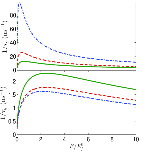
Figure 1: Plots of the inverse relaxation time $1/\tau_{h/l}$ versus energy for the Coulomb impurity potential for three different semiconductors: AlSb (solid green), GaAs (dashed red) and InAs (dashed-dot blue).

For various plots, we have taken $n_{\rm imp}=10^{21}$ m^-3 and $n_{h}=5\times 10^{23}$ m^-3. In Fig. (1), we show the variations of $1/\tau_{h/l}(E)$ with the energy $E$ (in units of $E_{\rm f}^{0}$) for three different semiconductors. It clearly shows that $\tau_{h}(E)>\tau_{l}(E)$ due to huge mass difference between heavy and light holes. Using the results of the relaxation times at the Fermi energy, the variation of the Drude conductivity with the hole density is shown in Fig. 2.

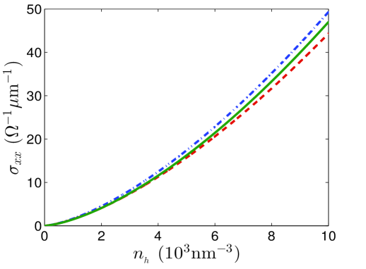
Figure 2: Plots of the Drude conductivity $\sigma_{xx}$ versus hole density $n_{h}$ for the Coulomb potential for three different semiconductors: AlSb (solid green), GaAs (dashed red) and InAs (dashed-dot blue).

In the Thomas-Fermi limit, $k_{s}^{\lambda}\gg k_{\rm f}^{\lambda}$, the Coulomb potential in momentum space can be approximated as $V_{\rm imp}^{\lambda}({\bf q})\simeq Ze^{2}/(\epsilon[k_{s}^{\lambda}]^{2})$. Within the Thomas-Fermi approximation, the inverse relaxation times are given by

$$\frac{1}{\tau_{\lambda}(E_{\rm f})}\simeq a_{\lambda}\frac{n_{\rm imp}m_{\lambda}}{16\pi\hbar^{3}}\Big{[}\frac{Ze^{2}}{\epsilon}\Big{]}^{2}\frac{k_{\rm f}^{\lambda}}{(k_{s}^{\lambda})^{4}},$$ (20)

where $a_{h}=8/5$ and $a_{l}=56/15$. The ratio between $\tau_{h}$ and $\tau_{l}$ is

$$\frac{\tau_{h}}{\tau_{l}}=\frac{7}{3}\Big{(}\frac{m_{h}}{m_{l}}\Big{)}^{3/2}=\frac{7}{3}\Big{[}\frac{\gamma_{1}+2\gamma_{2}}{\gamma_{1}-2\gamma_{2}}\Big{]}^{3/2}.$$ (21)

This ratio depends solely on the Luttinger parameters and clearly indicates that $\tau_{h}>\tau_{l}$. The Drude conductivity in Thomas-Fermi regime is given by

$$\sigma_{xx}\simeq\frac{n_{h}e^{2}\tau_{B}}{m_{0}}\frac{16k_{\rm f}^{0}}{\pi^{3}a_{B}^{2}n_{\rm imp}}\frac{a_{h}^{\prime}(\gamma_{1}+2\gamma_{2})^{2}+a_{l}^{\prime}(\gamma_{1}-2\gamma_{2})^{2}}{\big{[}(\gamma_{1}-2\gamma_{2})^{3/2}+(\gamma_{1}+2\gamma_{2})^{3/2}\big{]}^{4/3}},$$

where $\tau_{B}=(4\pi\epsilon/Ze^{2})^{2}(\hbar^{3}/m_{0})$, $a_{B}=4\pi\epsilon\hbar^{2}/(Ze^{2}m_{0})$ and $a_{h/l}^{\prime}=1/a_{h/l}$. The above equation depicts that the density dependence of the Drude conductivity due to the Coulomb impurity potential is $n_{h}^{4/3}$.

ii) Gaussian impurity potential: The Gaussian impurity potential is taken as $V^{\lambda}({\bf r})=V_{0}e^{-(k_{s}^{\lambda}r)^{2}/2}$ with $V_{0}$ is the strength of the potential. Its Fourier transform is $V^{\lambda}({\bf q})=V_{0}(\sqrt{2\pi}/k_{s}^{\lambda})^{3}e^{-q^{2}/(\sqrt{2}k_{s}^{\lambda})^{2}}$. Following the same method as described above, the inverse relaxation times for heavy and light holes are given by

$$\frac{1}{\tau_{h}({\bf k})}=\frac{n_{\rm imp}\pi^{2}m_{h}V_{0}^{2}k}{2\hbar^{3}(k_{s}^{h})^{6}}\int_{0}^{\pi}d\theta^{\prime}\sin^{3}\theta^{\prime}(1+\cos\theta^{\prime})^{2}e^{-(q/k_{s}^{h})^{2}}$$

and

$$\frac{1}{\tau_{l}({\bf k})}=\frac{n_{\rm imp}\pi^{2}m_{l}V_{0}^{2}k}{2\hbar^{3}(k_{s}^{l})^{6}}\int_{0}^{\pi}d\theta^{\prime}\sin^{3}\theta^{\prime}(3\cos\theta^{\prime}-1)^{2}e^{-(q/k_{s}^{l})^{2}},$$

where $q^{2}=2k^{2}(1-\cos\theta^{\prime})$. After performing the angular integral, the inverse relaxation time for heavy and light holes are given by

$$\frac{\tau_{0}}{\tau_{h}(E)} = \frac{\sqrt{\gamma_{1}-2\gamma_{2}}(\gamma_{1}^{2}-4\gamma_{2}^{2})E^{-9/2}}{[(\gamma_{1}-2\gamma_{2})^{3/2}+(\gamma_{1}+2\gamma_{2})^{3/2}]^{2/3}}A_{h}(E)$$

$$\frac{\tau_{0}}{\tau_{l}(E)} = \frac{\sqrt{\gamma_{1}+2\gamma_{2}}(\gamma_{1}^{2}-4\gamma_{2}^{2})E^{-9/2}}{[(\gamma_{1}-2\gamma_{2})^{3/2}+(\gamma_{1}+2\gamma_{2})^{3/2}]^{2/3}}B_{h}(E).$$

Here, $A_{h}(E)=3(1+d_{h}E)e^{-4d_{h}E}+(-3+d_{h}E(9+4d_{h}E(-3+2d_{h}E)))$, $B_{h}(E)=-27+45d_{l}E-28(d_{l}E)^{2}+(2d_{l}E)^{3}+[27+63d_{l}E+(8d_{l}E)^{2}+32(d_{l}E)^{3})]e^{-4d_{l}E}$ and $1/\tau_{0}=\Big{[}\frac{Ze^{2}}{4\pi\epsilon}\Big{]}^{2}\frac{n_{\rm imp}V_{0}^{2}}{\sqrt{32m_{0}}(E_{\rm f}^{0})^{7/2}}$.

The variations of $1/\tau_{h/l}(E)$ versus energy $E/E_{\rm f}^{0}$ for the Gaussian impurity potential for three different semiconductors are shown in Fig. 3. It clearly shows that $\tau_{h}(E)>\tau_{l}(E)$ due to huge mass difference between heavy and light holes. Using the results of the relaxation time at the Fermi energy, the variation of the Drude conductivity with the hole density for Gaussian scattering potential is shown in Fig. 4.

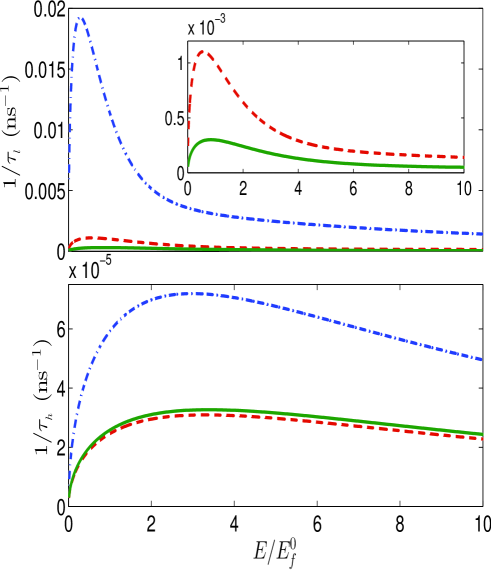
Figure 3: Plots of the inverse relaxation time $1/\tau_{h/l}$ versus $E/E_{\rm f}^{0}$ for the Gaussian impurity potential for three different semiconductors: AlSb (solid green), GaAs (dashed red) and InAs (dashed-dot blue). Here, we have taken $V_{0}=0.1$ meV.

In the Thomas-Fermi limit, $k_{s}^{\lambda}\gg k_{\rm f}^{\lambda}$, the Gaussian impurity potential in momentum space can be approximated as $V_{\rm imp}^{\lambda}({\bf q})\simeq V_{0}(\sqrt{2\pi}/k_{s}^{\lambda})^{3}$. Within the Thomas-Fermi approximation, the inverse relaxation times at the Fermi level are given by

$$\frac{1}{\tau_{\lambda}(E_{\rm f})}\simeq a_{\lambda}\frac{n_{\rm imp}\pi^{2}m_{\lambda}V_{0}^{2}k_{\rm f}^{\lambda}}{2\hbar^{3}(k_{s}^{\lambda})^{6}}.$$ (22)

The ratio between $\tau_{h}$ and $\tau_{l}$ is

$$\frac{\tau_{h}}{\tau_{l}}=\frac{7}{3}\Big{(}\frac{m_{h}}{m_{l}}\Big{)}^{3}=\frac{7}{3}\Big{[}\frac{\gamma_{1}+2\gamma_{2}}{\gamma_{1}-2\gamma_{2}}\Big{]}^{3}.$$ (23)

This ratio depends solely on the Luttinger parameters and clearly indicates that $\tau_{h}>\tau_{l}$. Moreover, the ratio $\tau_{h}/\tau_{l}$ for the Gaussian impurity potential is large as compared to the ratio for the Coulomb impurity potential. The Drude conductivity in the Thomas-Fermi regime is given by

$$\sigma_{xx} = \frac{n_{h}e^{2}\tau_{B}}{m_{0}}\frac{256\hbar^{2}E_{\rm f}^{0}}{\pi^{5}V_{0}^{2}n_{\rm imp}m_{0}a_{B}^{5}}$$

$$\times \frac{a_{h}^{\prime}(\gamma_{1}+2\gamma_{2})^{7/2}+a_{l}^{\prime}(\gamma_{1}-2\gamma_{2})^{7/2}}{[(\gamma_{1}+2\gamma_{2})^{3/2}+(\gamma_{1}-2\gamma_{2})^{3/2}]^{5/3}(\gamma_{1}^{2}-4\gamma_{2}^{2})}.$$

The density dependence of the Drude conductivity due to the Gaussian impurity potential is $n_{h}^{5/3}$.

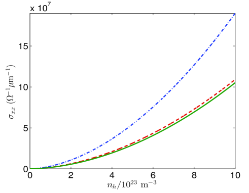
Figure 4: Plots of the Drude conductivity $\sigma_{xx}$ versus hole density $n_{h}$ for the Gaussian potential for three different semiconductors: AlSb (solid green), GaAs (dashed red) and InAs (dashed-dot blue). Here, we have taken $V_{0}=0.1$ meV.

iii) Short-range impurity potential: The short-range impurity potential is considered as $U({\bf r})=U_{0}\delta({\bf r}-{\bf r}_{i})$, with $U_{0}$ has the dimension of energy times volume and ${\bf r}_{i}$ is the position of the $i$-th impurity. Following the same method, the energy variation of the inverse relaxation times for short-range impurity potential are obtained as

$$\frac{1}{\tau_{h}(E)} = \frac{m_{h}^{3/2}n_{\rm imp}U_{0}^{2}}{10\pi\hbar^{4}}\sqrt{2E},$$ (24)

$$\frac{1}{\tau_{l}(E)} = \frac{7m_{l}^{3/2}n_{\rm imp}U_{0}^{2}}{30\pi\hbar^{4}}\sqrt{2E}.$$ (25)

The ratio between $\tau_{h}$ and $\tau_{l}$ is $\tau_{h}/\tau_{l}=(7/3)(m_{h}/m_{l})^{3/2}=(7/3)[(\gamma_{1}+2\gamma_{2})/(\gamma_{1}-2\gamma_{2})]^{3/2}.$ It shows that $\tau_{h}<\tau_{l}$ and is just opposite to the long-range impurity potentials cases. The Drude conductivity is given by

$$\sigma_{xx}=\frac{a_{0}e^{2}\hbar^{3}n_{h}^{2/3}}{n_{\rm imp}m_{0}U_{0}^{2}}\frac{(5\gamma_{1}+4\gamma_{2})}{\big{[}(\gamma_{1}-2\gamma_{2})^{3/2}+(\gamma_{1}+2\gamma_{2})^{3/2}\big{]}^{2/3}},$$

with $a_{0}=20\pi/(3(3\pi^{2})^{1/3})$. The Drude conductivity for the short-range potential varies with the carrier density as $n_{h}^{2/3}$.

Keeping in mind that $E_{\rm f}\approx 2E_{\rm f}^{0}$, the $1/\tau_{l}$ increases with the energy $E$, peaks at certain value $E\ll E_{\rm f}$, and then decreases rapidly while $E$ approaches to $E_{\rm f}$ for the Coulomb as well as the Gaussian impurity potentials. On the other hand, $1/\tau_{h}$ increases with energy $E$, peaks in and around $E_{\rm f}$ and then decreases slowly when $E\gg E_{\rm f}$ for the Coulomb and the Gaussian impurity potentials. For the short-range impurity potential, $1/\tau_{h/l}$ always increases with the energy as $\sqrt{E}$.

IV Drude weight and Optical conductivity

An oscillating electric field with zero-momentum ${\bf E}=E_{x}e^{i\omega t}\hat{\bf x}$ is applied on the spin-split hole gas in $p$-doped bulk III-V semiconductors. The complex charge conductivity is given by

$$\Sigma_{xx}(\omega)=\sigma_{D}(\omega)+\sigma_{xx}(\omega).$$ (26)

Here $\sigma_{D}(\omega)=\sum_{\lambda}\sigma_{xx}^{\lambda}/(1-i\omega\tau_{\lambda})$ is the dynamic Drude conductivity arises from the intra-band transitions, with $\sigma_{xx}^{\lambda}$ being the static Drude conductivity which is derived in the previous section. Also, $\sigma_{xx}(\omega)$ is the complex conductivity arises from the interband optical transitions between heavy hole and light hole states. The absorptive parts of the optical transitions correspond to the real parts of the complex optical conductivities $\sigma_{D}$ and $\sigma_{xx}(\omega)$. The minima in the experimentally observed spectra correspond to the peaks in the real part of the conductivities.

Drude weight: The real part of the dynamic Drude conductivity is ${\rm Re}\,[\sigma_{D}(\omega)]=D_{w}\delta(\omega)$, where $D_{w}=\pi\sum_{\lambda}\sigma_{xx}^{\lambda}/\tau_{\lambda}$ is called the zero-frequency Drude weight, whose peak is centered around $\omega=0$. Using Eq. (16) for $\sigma_{xx}$, the Drude weight is given by

$$D_{w}=\frac{\pi n_{h}e^{2}}{m_{0}}\bigg{[}\gamma_{1}+2\gamma_{2}\frac{(\gamma_{1}-2\gamma_{2})^{3/2}-(\gamma_{1}+2\gamma_{2})^{3/2}}{(\gamma_{1}-2\gamma_{2})^{3/2}+(\gamma_{1}+2\gamma_{2})^{3/2}}\bigg{]}.$$ (27)

The Drude weight is linearly varying with the carrier density $n_{h}$ as expected since the full Hamiltonian is quadratic in momentum.

Optical conductivity: Within the framework of linear response theory, the Kubo formula for the optical conductivity is given by

$$\sigma_{\mu\nu}(\omega)=\frac{1}{\hbar(\omega-i\eta)}\int_{0}^{\infty}dt\textrm{ }\mathrm{e}^{(i(\omega+i\eta)t)}\langle[\hat{j}_{\mu}(t),\hat{j}_{\nu}(0)]\rangle,$$ (28)

where $(\mu,\nu=x,y,z)$, $\hat{j}_{\mu}=e\hat{v}_{\mu}$ is the charge current density operator. The quantity

$$\langle[\hat{j}_{\mu}(t),\hat{j}_{\nu}(0)]\rangle = \sum_{\lambda,\lambda^{\prime}}\int d^{3}{\bf k}f(E_{\lambda}({\bf k}))\langle{\bf k}\lambda^{\prime}\big{|}[\hat{j}_{\mu}(t),\hat{j}_{\nu}(0)]\big{|}{\bf k}\lambda\rangle$$ (29)

$$= \sum_{\lambda,\lambda^{\prime}}\Big{[}f(E_{\lambda}({\bf k}))-f(E_{\lambda^{\prime}}({\bf k}))\Big{]}$$

$$\times \mathrm{e}^{i(E_{\lambda}({\bf k})-E_{\lambda^{\prime}}({\bf k}))t/\hbar}j_{\mu}^{\lambda,\lambda^{\prime}}j_{\nu}^{\lambda^{\prime},\lambda}$$

with $f(\epsilon)=1/(\exp[\beta(\epsilon-\epsilon_{f})]+1)$ being the Fermi distribution function and $j_{\mu}^{\lambda,\lambda^{\prime}}=ev_{\mu}^{\lambda,\lambda^{\prime}}=e\langle\lambda|\hat{v}_{\mu}|\lambda^{\prime}\rangle$. Using the above mention results, the absorptive part of $\sigma_{xx}(\omega)$ is simplified to

$$\textrm{Re}\,[\sigma_{xx}(\omega)] = -\frac{e^{2}}{8\pi^{2}\omega}\sum_{\lambda,\lambda^{\prime}}\int d^{3}k\Big{[}f(E_{\lambda}({\bf k}))-f(E_{\lambda^{\prime}}({\bf k}))\Big{]}v_{x}^{\lambda,\lambda^{\prime}}({\bf k})v_{x}^{\lambda^{\prime},\lambda}({\bf k})\delta\big{(}E_{\lambda}({\bf k})-E_{\lambda^{\prime}}({\bf k})-\hbar\omega\big{)}$$ (30)

$$= -\frac{e^{2}}{2\pi^{2}\omega}\int d^{3}k\Big{[}f(E_{l}({\bf k}))-f(E_{h}({\bf k}))\Big{]}v_{x}^{l,h}({\bf k})v_{x}^{h,l}({\bf k})\delta(E_{l}({\bf k})-E_{h}({\bf k})-\hbar\omega)+(h\longleftrightarrow l).$$

It is to be noted that a factor 4 has been multiplied to obtain Eq. (30). This is the results of the 2-fold degeneracy of the light and heavy holes. Using the following results $v_{x}^{h,l}({\bf k})=[v_{x}^{l,h}]^{*}=-\sqrt{3}\gamma_{2}(\hbar k/m_{0})\big{[}\cos\theta\cos\phi+i\sin\phi\big{]}$, we can re-write Eq. (30) as

$$\textrm{Re}\,[\sigma_{xx}(\omega)] = \frac{3e^{2}}{2\pi^{2}\omega}\gamma_{2}^{2}\frac{\hbar^{2}}{m_{0}^{2}}\int d^{3}k\,k^{2}(\cos^{2}\theta\cos^{2}\phi+\sin^{2}\phi)\delta\Big{(}\frac{2\gamma_{2}\hbar^{2}k^{2}}{m_{0}}-\hbar\omega\Big{)}\Big{[}f(E_{h}(k))-f(E_{l}(k))\Big{]}$$ (31)

$$= \frac{e^{2}}{h}k_{\omega}\big{[}f(E_{h}(k_{\omega}))-f(E_{l}(k_{\omega}))\big{]},$$

where $k_{\omega}=\sqrt{m_{0}\omega/2\gamma_{2}\hbar}$. An alternate derivation of the optical conductivity using the Green’s function technique is given in Appendix.

At $T=0$ K, the above equation can be written as

$$\textrm{Re}\,[\sigma_{xx}(\omega)] = \frac{e^{2}}{h}k_{\omega}\Theta(\hbar\omega-\epsilon_{l})\Theta(\epsilon_{h}-\hbar\omega),$$ (32)

where $\epsilon_{h/l}=2\gamma_{2}[\hbar k_{\rm f}^{h/l}]^{2}/m_{0}$ and $\Theta(x)$ is the unit step function.

In order to have interband transitions from heavy hole band to light hole band at $T=0$, the photon energy must follow the inequality $2\gamma_{2}[\hbar k_{\rm f}^{l}]^{2}/m_{0}\leq\hbar\omega\leq 2\gamma_{2}[\hbar k_{\rm f}^{h}]^{2}/m_{0}$. With this, the magnitude of the optical conductivity at the left and right edges can be simply expressed as

$$\textrm{Re}\,[\sigma_{xx}(\omega_{L/R})]=\frac{e^{2}}{h}k_{\rm f}^{0}\frac{\sqrt{\gamma_{1}\pm 2\gamma_{2}}}{[(\gamma_{1}+2\gamma_{2})^{3/2}+(\gamma_{1}-2\gamma_{2})^{3/2}]^{1/3}},$$

where $\omega_{L/R}=\epsilon_{h/l}/\hbar=2\gamma_{2}\hbar[k_{\rm f}^{h/l}]^{2}/m_{0}$. The optical band width (region in which $\sigma_{xx}(\omega)$ remains finite) is given by

$$\Delta_{\rm op}=\frac{(4\gamma_{2})^{2}E_{\rm f}^{0}}{[(\gamma_{1}+2\gamma_{2})^{3/2}+(\gamma_{1}-2\gamma_{2})^{3/2}]^{2/3}}.$$ (33)

The band width $\Delta_{\rm op}$ and $\textrm{Re}\,[\sigma_{xx}(\omega_{L/R})]$ goes as $n_{h}^{2/3}$ and $n_{h}^{1/3}$, respectively.

In Fig. 5, we plot the optical conductivity versus photon energy for three different III-V semiconductors at $T=0$.

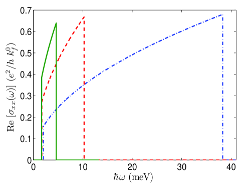
Figure 5: Plots of the absorptive part of the optical conductivity (in units of $(e^{2}/h$ $k_{f}^{0})$) versus photon energy for three different semiconductors: AlSb (solid green), GaAs (dashed red) and InAs (dashed-dot blue).

Table 1: Values of $\tau_{h/l},\epsilon_{h/l}$ and the Drude conductivity (in units of ($\Omega^{-1}$ $\mu$m^-1) along with the Luttinger parameters for six different III-V semiconductors.

III-V	$\gamma_{1}$	$\gamma_{2}$	$\sigma$	$\tau_{l}$ (ns)	$\tau_{h}$ (ns)	$\epsilon_{h}$ (meV)	$\epsilon_{l}$ (meV)
GaAs	7	2.5	15.703	0.062	0.571	10.262	1.710
InAs	20	9	17.383	0.025	0.619	38.295	2.015
InSb	35	15	36.457	0.057	0.513	63.439	4.879
AlSb	5.24	1.23	16.221	0.115	0.435	4.628	1.671
AlAs	3.84	1.71	11.439	0.021	0.185	7.267	0.420
GaSb	13.4	4.7	26.759	0.091	0.472	19.228	3.373

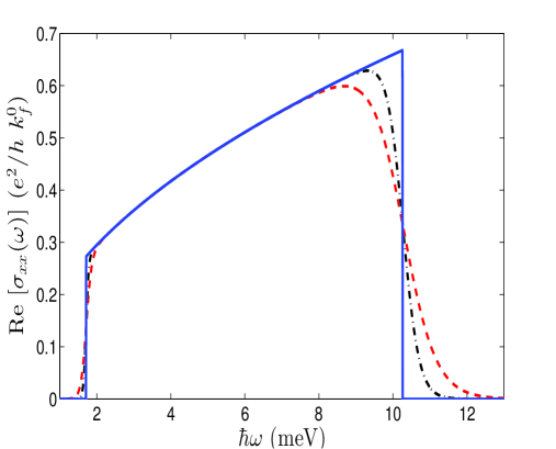
Figure 6: Plots of the absorptive part of the optical conductivity versus photon energy for GaAs at three different temperatures: $T=0$ K (solid blue), $T=0.5$ K (dot-dashed green) and $T=1$ K (dashed red).

We show the optical conductivity at three different temperature in Fig. 6. It is easy to see that at the two edges the conductivity is ${\rm Re}\,[\sigma_{xx}(\omega_{L/R})]/2$. The location of the onset of optical transition and the magnitude of the optical conductivity at this location do not change appreciably with the temperature. The Luttinger parameters $\gamma_{1}$ and $\gamma_{2}$ can be obtained from the onset energy $\epsilon_{l}$ and ${\rm Re}\,[\sigma_{xx}(\omega_{L})]$. Thus, an approximate values of the Luttinger parameters can be obtained from the experimental measurement of the optical conductivity. It should be noted here that a precise determination of the Luttinger parameters requires a proper analysis of the $6\times 6$ Luttinger Hamiltonian.

V Conclusion

In this work, we have presented detailed analysis of the electrical and optical conductivities of hole gas in $p$-doped bulk III-V semiconductors described by the $4\times 4$ Luttinger Hamiltonian. The exact analytical expressions of the Drude conductivity, inverse relaxation times for various impurity potentials, Drude weight and the optical conductivity are obtained. We find that the back scattering is completely suppressed due to the helicity conservation of the heavy hole and light hole states. The variation of the relaxation time with energy of the hole states is different from the Brooks-Herring formula for electron gas in $n$-doped semiconductors. It is shown that the relaxation time of heavy holes is much larger than that of the light holes for long-range impurity potentials and vice-versa for the short-range impurity potential. Note that our results are valid as long as the Fermi energy is smaller than the split-off energy. For more accurate results, one need to consider the $6\times 6$ Luttinger Hamiltonian. The effective masses of the HH and LH bands described by the $6\times 6$ Luttinger Hamiltonian will be different from the HH and LH bands described by the $4\times 4$ Hamiltonian. The effective band mass appears in the density of states and consequently in the inverse relaxation time as well as in the Drude conductivity. There will be a quantitative change in the inverse relaxation time and the Drude conductivity if we consider $6\times 6$ Luttinger Hamiltonian.

The Drude weight has a linear density dependency even with the non-zero spin-orbit coupling, due to $k^{2}$ dependence of the spin-orbit coupling. The finite-frequency optical conductivity is having $\sqrt{\omega}$ dependence. The onset energy for triggering optical transition and the amplitude of the optical conductivity at the onset energy depend on the Luttinger parameters $\gamma_{1}$ and $\gamma_{2}$. Therefore, the Luttinger parameters $\gamma_{1}$ and $\gamma_{2}$ can be determined approximately from the optical measurements. The values of the Luttinger parameters, $\tau_{h/l}$ at the Fermi energy for the Coulomb-type impurity potential, Drude conductivity at $T=0$ for the Coulomb-type impurity potential, onset energy $\epsilon_{h}$ and offset energy $\epsilon_{l}$ for the optical transition for six different III-V semiconductors are tabulated in Table 1.

Appendix A Alternative derivation of the optical conductivity

Here we shall provide alternative derivation of the optical conductivity. Using the Kubo formula, the optical conductivity can also be written as

$$\sigma_{xx}(\omega)=-\frac{e^{2}}{i\omega}\frac{1}{(2\pi)^{3}}\int_{0}^{\infty}\int_{0}^{\pi}\int_{0}^{2\pi}k^{2}\sin\theta dkd\theta d\phi$$ (34)

$$\times T\sum_{s}\textrm{Tr}\langle\hat{v}_{x}\hat{G}({\bf k},\omega_{s})\hat{v}_{x}\hat{G}({\bf k},\omega_{s}+\omega_{n})\rangle_{i\omega_{n}\rightarrow\omega+i\delta}.$$

Here $T$ is the temperature, $s$ and $n$ are integers, $\omega_{n}=(2n+1)\pi T$ and $\omega_{s}=2s\pi T$ are the fermionic and bosonic Matsubara frequencies, respectively.

The Green’s function of the Luttinger Hamiltonian [Eq. (2)] is given by

$$\hat{G}({\bf k},\omega_{n}) = \sum_{\lambda}\begin{bmatrix}-\frac{1}{2}-\lambda\frac{1+3\cos 2\theta}{8}&-\lambda\frac{\sqrt{3}}{4}\sin 2\theta\mathrm{e}^{-i\phi}&-\lambda\frac{\sqrt{3}}{4}\sin^{2}\theta\mathrm{e}^{-i2\phi}&0\\ -\lambda\frac{\sqrt{3}}{4}\sin 2\theta\mathrm{e}^{i\phi}&-\frac{1}{2}+\lambda\frac{1+3\cos 2\theta}{8}&0&-\lambda\frac{\sqrt{3}}{4}\sin^{2}\theta\mathrm{e}^{-i2\phi}\\ -\lambda\frac{\sqrt{3}}{4}\sin^{2}\theta\mathrm{e}^{i2\phi}&0&-\frac{1}{2}+\lambda\frac{1+3\cos 2\theta}{8}&-\lambda\frac{\sqrt{3}}{4}\sin 2\theta\mathrm{e}^{-i\phi}\\ 0&-\lambda\frac{\sqrt{3}}{4}\sin^{2}\theta\mathrm{e}^{i2\phi}&-\lambda\frac{\sqrt{3}}{4}\sin 2\theta\mathrm{e}^{i\phi}&-\frac{1}{2}-\lambda\frac{1+3\cos 2\theta}{8}\end{bmatrix}G_{0}^{\lambda}({\bf k},\omega_{n}),$$ (35)

where $G_{0}^{\lambda}({\bf k},\omega_{n})=1/(E_{\lambda}-\mu-i\hbar\omega_{n}).$ Using Eqs. (12) and (35), one can obtain

$$\textrm{Tr}\langle\hat{v}_{x}\hat{G}({\bf k},\omega_{s})\hat{v}_{x}\hat{G}({\bf k},\omega_{s}+\omega_{n})\rangle=\Big{\{}[2\gamma_{1}^{2}(1+\lambda\lambda^{\prime})-8\gamma_{1}\gamma_{2}(\lambda+\lambda^{\prime})]\cos^{2}\phi+\gamma_{2}^{2}\big{[}13+(7\lambda\lambda^{\prime}+1)\cos 2\phi-5\lambda\lambda^{\prime}\big{]}$$ (36)

$$+ 2\big{[}4\gamma_{1}\gamma_{2}(\lambda+\lambda^{\prime})-\gamma_{1}^{2}(1+\lambda\lambda^{\prime})-\gamma_{2}^{2}(1+7\lambda\lambda^{\prime})\big{]}\cos 2\theta\cos^{2}\phi\Big{\}}\Big{(}\frac{\hbar k}{2m_{0}}\Big{)}^{2}G_{0}^{\lambda}({\bf k},\omega_{n})G_{0}^{\lambda^{\prime}}({\bf k},\omega_{n}+\omega_{s}).$$

The identity

$$T\sum_{s}\bigg{[}\frac{1}{i\hbar\omega_{s}+\mu-E_{\lambda}}\frac{1}{i\hbar(\omega_{n}+\omega_{s})+\mu-E_{\lambda^{\prime}}}\bigg{]}$$ (37)

$$= \begin{cases}\frac{f(E_{\lambda})-f(E_{\lambda^{\prime}})}{i\hbar\omega_{n}-E_{\lambda^{\prime}}+E_{\lambda}},&\text{if }\lambda\neq\lambda^{\prime}\\ 0,&\text{otherwise.}\end{cases}$$

shows that there is no intra-band contribution to the optical conductivity. Thus by keeping only the terms involving inter-band transitions, we have

$$T\sum_{s}\textrm{Tr}\langle v_{x}\hat{G}({\bf k},\omega_{s})v_{x}\hat{G}({\bf k},\omega_{n}+\omega_{s})\rangle$$ (38)

$$= 6\Big{(}\frac{\gamma_{2}\hbar k}{m_{0}}\Big{)}^{2}\Big{[}\cos^{2}\theta\cos^{2}\phi+\sin^{2}\phi\Big{]}$$

$$\times \Big{[}\frac{f(E_{h})-f(E_{l})}{i\hbar\omega_{n}-E_{l}+E_{h}}\Big{]}+(E_{h}\leftrightarrow E_{l}).$$

It is to be noted that the second term turns out to be zero as a result of the conservation of energy.

Using the result of Eq. (38) in Eq. (34), we have

$$\sigma_{xx}(\omega)=-\frac{e^{2}}{i\omega}\frac{1}{(2\pi)^{3}}\int_{0}^{\infty}\int_{0}^{\pi}\int_{0}^{2\pi}k^{2}dk\sin\theta d\theta d\phi$$ (39)

$$\times 6\Big{(}\frac{\gamma_{2}\hbar k}{m_{0}}\Big{)}^{2}\Big{[}\cos^{2}\theta\cos^{2}\phi+\sin^{2}\phi\Big{]}$$

$$\times \Big{[}\frac{f(E_{h})-f(E_{l})}{i\hbar\omega_{n}-E_{l}+E_{h}}\Big{]}+(E_{h}\leftrightarrow E_{l})_{i\omega_{n}\rightarrow\omega+i\delta}.$$

On further simplification the absorptive part of the optical conductivity reduces to

$$\textrm{Re}\,[\sigma_{xx}(\omega)] = \frac{3e^{2}}{2\pi^{2}\omega}\gamma_{2}^{2}\frac{\hbar^{2}}{m_{0}^{2}}\int d^{3}k\,k^{2}(\cos^{2}\theta\cos^{2}\phi+\sin^{2}\phi)\delta\Big{(}\frac{2\gamma_{2}\hbar^{2}k^{2}}{m_{0}}-\hbar\omega\Big{)}\Big{[}f(E_{h}(k))-f(E_{l}(k))\Big{]}$$ (40)

$$= \frac{e^{2}}{h}k_{\omega}\big{[}f(E_{h}(k_{\omega}))-f(E_{l}(k_{\omega}))\big{]}.$$

References

- (1) J. M. Luttinger, Phys. Rev. 102, 1030 (1956)
- (2) S. Murakami, N. Nagaosa, and S. C. Zhang, Science 301, 1348 (2003)
- (3) Y. K. Kato, R. C. Myers, A. C. Gossard, and D. D. Awschalom, Science 306, 1910 (2004)
- (4) J. Wunderlich, B. Kaestner, J. Sinova, and T. Jungwirth, Phys. Rev. Lett. 94, 047204 (2005)
- (5) S. Murakami, N. Nagaosa, and S. C. Zhang, Phys. Rev. B 69, 235206 (2004)
- (6) Z. F. Jiang, R. D. Li, S.-C. Zhang, and W. M. Liu, Phys. Rev. B 72, 045201 (2005)
- (7) R. Winkler, U. Zulicke, and J. Bolte, Phys. Rev. B 75, 205314 (2007)
- (8) V. Ya. Demikhovskii, G. M. Maksimova, and E. V. Frolova, Phys. Rev. B 81, 115206 (2010)
- (9) J. Schliemann, Phys. Rev. B 74, 045214 (2006)
- (10) J. Schliemann, Euro. Phys. Lett 91, 67004 (2010)
- (11) J. Schliemann, Phys. Rev. B 84, 155201 (2011)
- (12) T. Dietl, H. Ohno, F. Matsukura, J. Cibert, and D. Ferrand, Science 287, 1019 (2000)
- (13) J. Sinova, T. Jungwirth, S.-R. Eric Yang, J. Kucera, and A. H. MacDonald, Phys. Rev. B 66, 041202 (2002)
- (14) Y. Nagai, T. Kunimoto, K. Nagasaka, H. Nojiri, M. Motokawa, F. Matsukura, T. Dietl, and H. Ohno, Jpn. J. Appl. Phys. 40, 6231 (2001)
- (15) S. Katsumoto, T. Hayashi, Y. Hashimoto, Y. Iye, Y. Ishiwata, M. Watanabe, R. Eguchi, T. Takeuchi, Y. Harada, and S. Shin, Mater. Sci. Eng., B 84, 88 (2001)
- (16) K. Hirakawa, S. Katsumoto, T. Hayashi, Y. Hashimoto, and Y. Iye, Phys. Rev. B 65, 193312 (2002)
- (17) K. W. Edmonds, P. Boguslawski, K. Y. Wang, R. P. Campion, S. N. Novikov, N. R. S. Farley, B. L. Gallagher, C. T. Foxon, M. Sawicki, T. Dietl, M. B. Nardelli, and J. Bernholc, Phys. Rev. Lett. 92, 037201, (2004)
- (18) T. Jungwirth, K. Y. Wang, J. Masek, K. W. Edmonds, J. König, J. Sinova, M. Polini, N. A. Goncharuk, A. H. MacDonald, M. Sawicki, R. P. Campion, L. X. Zhao, C. T. Foxon, and B. L. Gallagher, Phys. Rev. B 72, 165204 (2005)
- (19) T. Jungwirth, J. Sinova, J. Masek, J. Kucera, and A. H. MacDonald, Rev. Mod. Phys. 78, 809, (2006)
- (20) Jun-Won Rhim and Y. B. Kim, Phys. Rev. B 91, 115124 (2015)
- (21) C. H. Yang, W. Xu, Z. Zeng, F. Lu, and C. Zhang, Phys. Rev. B 74, 075321 (2006)
- (22) A. Mawrie and T. K. Ghosh, J. Appl. Phys. 119, 044303 (2016)
- (23) J. M. Luttinger and W. Kohn, Phys. Rev. 97, 869 (1955)
- (24) I. Vurgaftman, J. R. Meyer, and L. R. Ram-Mohan, J. Appl. Phys. 89, 5815 (2001)
- (25) N. W. Ashcroft and N. D. Mermin, Solid State Physics, (Harcourt College Publishes-2001)
- (26) T. Ando, T. Nakanishi, and R. Saito, J. Phys. Soc. Jpn. 67, 2857 (1998)
- (27) P. L. McEuen, M. Bockrath, D. H. Cobden, Y.-G. Yoon, and S. G. Louie, Phys. Rev. Lett. 83, 5098 (1999)
- (28) H. Brooks, Phys. Rev. 83, 879 (1951); H. Brooks, Advan. Electron. Electron Phys. 7, 85 (1955)