User Scheduling and Optimal Power Allocation
for Full-Duplex Cellular Networks

Abstract

The problem of user scheduling and power allocation in full-duplex (FD) cellular networks is considered, where a FD base station communicates simultaneously with one half-duplex (HD) user on each downlink and uplink channel. First, we propose low complexity user scheduling algorithms aiming at maximizing the sum rate of the considered FD system. Second, we derive the optimal power allocation for the two communication links, which is then exploited to introduce efficient metrics for FD/HD mode switching in the scheduling procedure, in order to further boost the system rate performance. We analyze the average sum rate of the proposed algorithms over Rayleigh fading and provide closed-form expressions. Our representative performance evaluation results for the algorithms with and without optimal power control offer useful insights on the interplay among rate, transmit powers, self-interference (SI) cancellation capability, and available number of users in the system.

I Introduction

Full-duplex (FD) communication is an emerging technology that has been recognized as one of the promising solutions to cope with the ever-growing demand for high data rates. FD systems allow simultaneous transmission and reception at the same time/frequency resource and have the potential to increase (theoretically double) the throughput in future (5G) wireless networks. There are two major challenges hindering the implementation of FD systems. First, the uplink (UL) communication is affected by the self-interference (SI) at the base station (BS), which is due to the signal leakage and imperfect isolation between transmit and receive antennas [1]. Second, the downlink (DL) communication suffers from the inter-user interference resulting from the UL mobile terminal (MT) using the same time/frequency resource.

Although resource allocation in half-duplex (HD) systems has been extensively studied, the new characteristics and challenges with FD communication have not been investigated yet. Without carefully allocating resources and selecting users, FD communication may cause excessive interference in both UL and DL, which may greatly limit the potential FD gains [2]. In this regard, [3] presents a distributed power allocation scheme for multi-cell FD scenarios that aims at maximizing the network throughput. A dynamic power control scheme in FD bidirectional networks was provided in [4]. In [5], a joint resource allocation problem including user pairing, subcarrier allocation, and power control for FD orthogonal division multiple access networks was considered. Low complexity user pairing algorithms that maximize the cell throughput or minimize the outage probability were presented in [6].

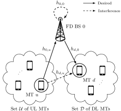
Figure 1: A small-cell FD cellular system with the desired and interfering channels at the receiving nodes.

In this work, we consider a FD BS communicating with one HD MT in the DL and one HD MT in the UL. We propose three low complexity user scheduling algorithms in order to maximize the system rate performance. In order to avoid the high complexity of inherent joint UL and DL scheduling, the selection procedure is decoupled and performed in two steps using efficient metrics. Furthermore, observing that for certain channel realizations, the HD mode in time-division duplex (TDD) outperforms the FD mode in terms of throughput, we derive a FD/HD switching method to further enhance the system rate. The switching metric is inspired by the optimal power allocation, which turns out to have a binary feature (e.g., as in [7] for the $2$-user interference channel). In addition, we provide closed-form expressions for the average sum rate of the proposed algorithms over Rayleigh fading channels. The main takeaway of this paper is that power control and low complexity user scheduling can boost the performance of FD small/pico cells [8] for realistic SI cancellation capabilities.

II System Model

Consider the scenario illustrated in Fig. 1, in which a small-cell FD BS communicates with a set $\mathcal{U}\triangleq\{1,2,\ldots,K_{\mathcal{U}}\}$ of HD MTs in the UL and a set $\mathcal{D}\triangleq\{1,2,\ldots,K_{\mathcal{D}}\}$ of DL HD MTs. In our system setup, the FD BS is indexed with $0$ and is equipped with one transmit and one receive antenna, whereas each MT has a single antenna. During a given time/ frequency resource unit, the BS schedules concurrently one MT from $\mathcal{U}$ and one MT from $\mathcal{D}$ so as to maximize the sum-rate performance; the selected UL and DL users are denoted as $u^{\star}\in\mathcal{U}$ and $d^{\star}\in\mathcal{D}$, respectively. The transmit powers of the BS and of every UL MT are denoted as $p_{0}\in[0,P_{0}]$ and $p_{\mathcal{U}}\in[0,P_{\mathcal{U}}]$, respectively, where $P_{0}$ and $P_{\mathcal{U}}$ represent the maximum powers for the DL and UL communications, respectively.

The narrowband complex-valued channel coefficient between a transmitting node $\ell\in\mathcal{U}\cup\{0\}$ and a receiving node $k\in\mathcal{D}\cup\{0\}$ is represented by $h_{k,\ell}$ and may include - in the general case - different propagation phenomena such as pathloss attenuation, small-scale fading, and shadowing. More specifically, $h_{0,u}$ represents the UL channel (i.e., between the BS $0$ and the $u$-th UL MT), $h_{d,0}$ denotes the DL channel (i.e., between the $d$-th DL MT and the BS $0$), $h_{d,u}$ is the inter-MT interference channel from the $u$-th UL MT to the $d$-th DL MT, and $h_{0,0}$ represents the residual SI channel seen at the receive antenna of the BS $0$ from its own transmit antenna due to the DL transmission. Assuming that the $u$-th UL MT and the BS are simultaneously transmitting, the baseband received signals at the BS $0$ and at the $d$-th DL MT can be mathematically expressed as

$$y_{0} \triangleq\sqrt{p_{\mathcal{U}}}h_{0,u}s_{u}+\sqrt{p_{0}}h_{0,0}s_{0}+n_{0},$$ (1)

$$y_{d} \triangleq\sqrt{p_{0}}h_{d,0}s_{0}+\sqrt{p_{\mathcal{U}}}h_{d,u}s_{u}+n_{d},$$ (2)

respectively, where $s_{\ell}$ denotes the unit power data symbol transmitted by node $\ell$ and $n_{k}$ is the additive complex white Gaussian noise (AWGN) with variance $\sigma_{k}^{2}$ at the receiving node $k$. The second summands in (1) and (2) represent the interference terms due to the BS FD operation mode (namely, the SI and the inter-MT interference); in the HD mode, both terms vanish.

III User Scheduling and Power Allocation

In this section, we first consider the case where fixed transmit powers are utilized for the concurrent UL and DL transmissions, and we propose three low complexity user scheduling algorithms. Then, we derive the optimal power allocation (OPA) between the UL and DL communications for maximizing the sum rate, which we exploit and incorporate in the user scheduling procedure to enhance its performance.

III-A User Scheduling Algorithms

Assuming fixed transmit powers $p_{0}$ and $p_{\mathcal{U}}$, and that all involved channel gains can be accurately estimated during an appropriately designed control plane, we present the following three low complexity user scheduling algorithms for the FD system under consideration.

• Received Signal Strength at both UL and DL (RSS-UL RSS-DL): The UL MT $u^{\star}$ and the DL MT $d^{\star}$ are selected as the ones with the highest channel gains in $\mathcal{U}$ and in $\mathcal{D}$, respectively (see Algorithm A1).

Algorithm A1 : RSS-UL RSS-DL User Scheduling

   Step 1  : Select the UL MT $u^{\star}$ such that:

$$u^{\star}=\operatornamewithlimits{argmax}_{u\in\mathcal{U}}|h_{0,u}|^{2}. \mathrm{A1.1}$$ ()

   Step 2  : Select the DL MT $d^{\star}$ such that:

$$d^{\star}=\operatornamewithlimits{argmax}_{d\in\mathcal{D}}|h_{d,0}|^{2}. \mathrm{A1.2}$$ ()

• Received Signal Strength at the UL and Signal-to-Interference-plus-Noise Ratio at the DL (RSS-UL SINR-DL): The UL MT $u^{\star}$ is selected first as the one with the highest channel gain in $\mathcal{U}$, and then the DL MT $d^{\star}$ is selected as the one experiencing the maximum SINR (see Algorithm A2).

Algorithm A2 : RSS-UL SINR-DL User Scheduling

   Step 1  : Select the UL MT $u^{\star}$ as in ($\mathrm{A1.1}$).

   Step 2  : Select the DL MT $d^{\star}$ such that:

$$d^{\star}=\operatornamewithlimits{argmax}_{d\in\mathcal{D}}\frac{p_{0}|h_{d,0}|^{2}}{p_{\mathcal{U}}|h_{d,u^{\star}}|^{2}+\sigma_{d}^{2}}. \mathrm{A2.1}$$ ()

• Received Signal Strength at the DL and Signal-to-Leakage-plus-Noise Ratio at the UL (RSS-DL SLNR-UL): The DL MT $d^{\star}$ is selected first as the one with the highest channel gain in $\mathcal{D}$, and then the UL MT $u^{\star}$ is selected as the one yielding the maximum SLNR, i.e., as the MT that simultaneously presents high UL channel gain and creates low inter-MT interference to the scheduled DL MT $d^{\star}$ (see Algorithm A3).

Algorithm A3 : RSS-DL SLNR-UL User Scheduling

   Step 1  : Select the DL MT $d^{\star}$ as in ($\mathrm{A1.2}$).

   Step 2  : Select the UL MT $u^{\star}$ such that:

$$u^{\star}=\operatornamewithlimits{argmax}_{u\in\mathcal{U}}\frac{p_{\mathcal{U}}|h_{0,u}|^{2}}{p_{\mathcal{U}}|h_{d^{\star},u}|^{2}+\sigma_{0}^{2}}. \mathrm{A3.1}$$ ()

Remark: In the Algorithm A1, the steps of selecting the UL MT $u^{\star}$ and the DL MT $d^{\star}$ do not affect each other and may, therefore, be performed independently. On the other hand, in the Algorithms A2 and A3, knowledge of the UL (respectively DL) MT channel gain is not required in the DL (respectively UL) scheduling step. In fact, once the UL MT $u^{\star}$ (respectively the DL MT $d^{\star}$) is selected, it suffices to know only $h_{d,u^{\star}}$ $\forall d\!\in\!\mathcal{D}$ (respectively $h_{d^{\star},u}$ $\forall u\!\in\!\mathcal{U}$) for the Algorithm A2 (respectively for the Algorithm A3), instead of $h_{d,u}$ $\forall d\!\in\!\mathcal{D}$ and $\forall u\!\in\!\mathcal{U}$.

III-B Optimal Power Allocation (OPA)

The user scheduling algorithms presented above assume that the system always operates in FD mode. However, in certain system configurations, i.e., for certain values of the intended channels and levels of the inter-MT interference, the system rate performance is maximized by operating in HD mode. For that, we hereinafter aim at determining the optimal transmit powers $p_{0}^{\star}$ and $p_{\mathcal{U}}^{\star}$ for the BS $0$ and for the scheduled UL MT $u^{\star}$, which maximize the instantaneous sum rate. The power allocation between the UL and DL transmissions is assumed to take place after selecting $u^{\star}$ and $d^{\star}$ using any of the user scheduling algorithms described in Section III-A.

Capitalizing on (1) and (2), the SINRs at the BS $0$ and at the scheduled DL MT $d^{\star}$ are given by

$$\gamma_{0} \triangleq\frac{p_{\mathcal{U}}|h_{0,u^{\star}}|^{2}}{p_{0}|h_{0,0}|^{2}+\sigma_{0}^{2}},$$ (3)

$$\gamma_{d^{\star}} \triangleq\frac{p_{0}|h_{d^{\star},0}|^{2}}{p_{\mathcal{U}}|h_{d^{\star},u^{\star}}|^{2}+\sigma_{d^{\star}}^{2}},$$ (4)

respectively. Hence, the instantaneous rates of the UL communication (i.e., of the link between the scheduled UL MT $u^{\star}$ and the BS $0$) and of the DL communication (i.e., of the link between the BS $0$ and the scheduled DL MT $d^{\star}$), measured in bps/Hz, can be computed as $\mathsf{R}_{0}\triangleq\log_{2}\left(1+\gamma_{0}\right)$ and $\mathsf{R}_{d^{\star}}\triangleq\log_{2}\left(1+\gamma_{d^{\star}}\right)$, respectively. The instantaneous rate $\mathsf{R}$ of the considered FD system is defined as the cumulative rate of the DL and UL communications, i.e., $\mathsf{R}\triangleq\mathsf{R}_{0}+\mathsf{R}_{d^{\star}}$. Using the latter definitions, we consider the OPA strategy that solves the following optimization problem:

$$\left(p_{0}^{\star},p_{\mathcal{U}}^{\star}\right)\triangleq\operatornamewithlimits{argmax}_{\begin{subarray}{c}p_{0}\in[0,P_{0}]\\ p_{\mathcal{U}}\in[0,P_{\mathcal{U}}]\end{subarray}}\mathsf{R}(p_{0},p_{\mathcal{U}}),$$ (5)

where we have highlighted the dependence of $\mathsf{R}$ on the powers of the DL and UL transmissions. Solving (5) yields the OPA strategy summarized below in Theorem 1; therein, we make use of the following function definitions for $x\geq 0$:

$$\zeta(x) \triangleq\frac{|h_{0,u^{\star}}|^{2}\sigma_{d^{\star}}^{2}}{x|h_{0,0}|^{2}+\sigma_{0}^{2}}-|h_{d^{\star},u^{\star}}|^{2},$$ (6)

$$\eta(x) \triangleq\frac{|h_{d^{\star},0}|^{2}\sigma_{0}^{2}}{x|h_{d^{\star},u^{\star}}|^{2}+\sigma_{d^{\star}}^{2}}-|h_{0,0}|^{2}.$$ (7)

Theorem 1.

Given $\zeta(p_{0})$ and $\eta(p_{\mathcal{U}})$ obtained from (6) and (7), respectively, the OPA strategy is determined as:

• If $\zeta(P_{0})\geq 0$ and $\eta(P_{\mathcal{U}})\geq 0$, then the optimal power allocation is given by $\left(p_{0}^{\star},p_{\mathcal{U}}^{\star}\right)=\left(P_{0},P_{\mathcal{U}}\right)$, i.e., FD mode with maximum transmit powers is optimal;

• If $\zeta(P_{0})<0$ and/or $\eta(P_{\mathcal{U}})<0$, then (5) is solved by either $\left(p_{0}^{\star},p_{\mathcal{U}}^{\star}\right)=\left(P_{0},P_{\mathcal{U}}\right)$ (i.e., FD mode with maximum transmit powers), or $\left(p_{0}^{\star},p_{\mathcal{U}}^{\star}\right)=\left(0,P_{\mathcal{U}}\right)$ (i.e., HD mode in the UL direction with maximum transmit power), or $\left(p_{0}^{\star},p_{\mathcal{U}}^{\star}\right)=\left(P_{0},0\right)$ (i.e., HD mode in the DL direction with maximum transmit power).

Proof:

See Appendix A. ∎

The OPA in the considered FD system has a remarkably simple nature, i.e., the power allocation maximizing the system rate performance is binary. This simple binary OPA is exploited in the scheduling procedure and is incorporated as an additional step in order to maximize the system performance by switching between the optimal operation modes, i.e., HD or FD mode. For the cases where the OPA strategy corresponds to HD mode, either in the UL or DL direction, one can repeat the scheduling of the UL or DL MT so as to maximize the HD rate: this corresponds to selecting the UL or DL MT as in ($\mathrm{A1.1}$) or ($\mathrm{A1.2}$), respectively, of Algorithm A1. The OPA strategy for user scheduling can be summarized as follows:

• User Scheduling with OPA: After selecting the UL MT $u^{\star}$ and the DL MT $d^{\star}$ with any of the user scheduling algorithms presented in Section III-A using the maximum allowable transmit powers, the FD/HD mode of operation that maximizes the system rate performance is determined. If the OPA yields the HD mode in the UL (respectively in the DL), then the UL MT $u^{\star}$ (respectively the DL MT $d^{\star}$) is recomputed so as to maximize the UL (respectively the DL) TDD communication rate (see Enhancement of A1–A3 on the top of this column).

Enhancement of A1–A3: User Scheduling with OPA

   Step 1  :  Run Algorithm A1, or A2, or A3 to obtain               $d^{\star}$ and $u^{\star}$.

   Step 2  : If $\eta(P_{0})\geq 0$ and $\zeta(P_{\mathcal{U}})\geq 0$, then

$$\left(p_{0}^{\star},p_{\mathcal{U}}^{\star}\right)=\left(P_{0},P_{\mathcal{U}}\right).$$

              Else

$$\hskip 41.82558pt\left(p_{0}^{\star},p_{\mathcal{U}}^{\star}\right)=\operatornamewithlimits{argmax}_{\begin{subarray}{c}p_{0}\in\{0,P_{0}\}\\ p_{\mathcal{U}}\in\{0,P_{\mathcal{U}}\}\end{subarray}}\mathsf{R}(p_{0},p_{\mathcal{U}}).$$

                  If $p_{0}^{\star}=0$, select $u^{\star}$ as in ($\mathrm{A1.1}$).                   Else If $p_{\mathcal{U}}^{\star}=P_{\mathcal{U}}$, select $d^{\star}$ as in ($\mathrm{A1.2}$).                   End              End

IV Sum-Rate Analysis
over Rayleigh Fading Channels

The average sum rate of the considered FD system with any of the user scheduling Algorithms A1–A3 presented in the previous section is defined as

$$\overline{\mathsf{R}} \triangleq\overline{\mathsf{R}}_{0}+\overline{\mathsf{R}}_{d^{\star}}$$ (8)

$$=\int_{0}^{\infty}\log_{2}(1+x)\big{(}f_{\gamma_{0}}(x)+f_{\gamma_{d^{\star}}}(x)\big{)}\mathrm{d}x$$

$$=\frac{1}{\log 2}\int_{0}^{\infty}\frac{2-F_{\gamma_{0}}(x)-F_{\gamma_{d^{\star}}}(x)}{x+1}\mathrm{d}x$$

where $\overline{\mathsf{R}}_{0}$ and $\overline{\mathsf{R}}_{d^{\star}}$ denote the average rates of the UL and DL communications, respectively, and notations $f_{\gamma}(\cdot)$ and $F_{\gamma}(\cdot)$ represent the probability density function (PDF) and the cumulative distribution function (CDF), respectively, of a random variable (RV) $\gamma$. In deriving the last step in (8) we have used the Stieltjes transform of the complementary CDFs.

In the following, we provide closed-form expressions of (8) for the Algorithms A1 and A2 under the following assumptions: i) all channels apart from $h_{0,0}$ are subject to Rayleigh fading with unit mean squared amplitude value; ii) the SI power $|h_{0,0}|^{2}$ is a constant real positive number; and iii) all the DL MTs have the same AWGN variance, i.e., $\sigma_{d}^{2}=\sigma_{\mathcal{D}}^{2}$ $\forall d\!\in\!\mathcal{D}$. Due to space limitations, we omit the rate analysis for Algorithms A3 and the user scheduling with OPA, which will be considered in a longer version of this paper. Note that the following results can be straightforwardly extended to the case where $h_{0,0}$ is subject to Ricean fading [1]. Before proceeding with the average rate expressions, we introduce the function $\xi_{n}(x,y)$, with $x,y\geq 0$ and integer $n>0$, defined as

$$\xi_{n}(x,y)\triangleq\frac{(-x)^{n-1}}{\Gamma(n)}\bigg{(}\sum_{k=1}^{n-1}\Gamma(k)(-x)^{-k}y^{-k}-e^{xy}{\rm Ei}(-xy)\bigg{)},$$ (9)

where ${\rm Ei}(\cdot)$ denotes the exponential integral function [9, Eq. (8.211/1)]; observe that, for $n=y=1$, we simply have $\xi_{1}(x,1)=-e^{x}{\rm Ei}(-x)$. Furthermore, we introduce the parameter $w_{n}\triangleq(1-p_{0}/p_{\mathcal{U}})^{-n}$.

Theorem 2.

The average sum rate of the considered FD system obtained with the Algorithm A1 is given by

$$\overline{\mathsf{R}}_{\rm A1}\triangleq\ \overline{\mathsf{R}}_{0}+\sum_{k=1}^{K_{\mathcal{D}}}\binom{K_{\mathcal{D}}}{k}\frac{\left(-1\right)^{k+1}}{\log 2}\left(\frac{p_{0}}{p_{0}-kp_{\mathcal{U}}}\right)$$ (10)

$$\times\left(\xi_{1}\left(\frac{k\sigma_{\mathcal{D}}^{2}}{p_{0}},1\right)-\xi_{1}\left(\frac{k\sigma_{\mathcal{D}}^{2}}{p_{0}},\frac{p_{0}}{kp_{\mathcal{U}}}\right)\right)$$

where $\overline{\mathsf{R}}_{0}$ is obtained as

$$\overline{\mathsf{R}}_{0}\triangleq\sum_{k=1}^{K_{\mathcal{U}}}\binom{K_{\mathcal{U}}}{k}\frac{\left(-1\right)^{k+1}}{\log 2}\xi_{1}\bigg{(}\frac{k\left(p_{0}|h_{0,0}|^{2}+\sigma_{0}^{2}\right)}{p_{\mathcal{U}}},1\bigg{)}.$$ (11)

Proof:

See Appendix B. ∎

Theorem 3.

The average sum rate of the considered FD system obtained with the Algorithm A2 is given by

$$\overline{\mathsf{R}}_{\rm A2}\triangleq\overline{\mathsf{R}}_{0}+\frac{1}{\log 2}\sum_{k=1}^{K_{\mathcal{D}}}\binom{K_{\mathcal{D}}}{k}\left(-\frac{p_{0}}{p_{\mathcal{U}}}\right)^{k}\bigg{(}\sum_{\ell=1}^{k}(-1)^{\ell}\bigg{.}$$ (12)

$$\times\bigg{.}w_{\ell}\xi_{k-\ell+1}\left(\frac{k\sigma_{\mathcal{D}}^{2}}{p_{0}},\frac{p_{0}}{p_{\mathcal{U}}}\right)\!+(-1)^{1-k}w_{k}\xi_{1}\left(\frac{k\sigma_{\mathcal{D}}^{2}}{p_{0}},1\right)\!\bigg{)}$$

where $\overline{\mathsf{R}}_{0}$ is defined in (11).

Proof:

See Appendix C. ∎

IV-A Sum-Rate Scaling and Multi-User Diversity

We next investigate the scaling law of the sum rate achieved by the proposed user scheduling algorithms in order to show their multi-user diversity gain. The asymptotic growth of the sum rate as the number of MTs goes to infinity, with fixed transmit powers, can be formally shown using the extreme value theory [10]. Using standard tools (e.g., Smirnov and Gnedenko theorems), we can easily show that the asymptotic limit distribution of the CDFs of both $\gamma_{0}$ and $\gamma_{d^{\star}}$ belongs to the Gumbel domain of attraction. Due to space limitation, we provide a less formal, yet insightful, analysis. We present results only for the Algorithm A1, as the sum-rate scaling of the Algorithms A2 and A3 can be derived in a similar way.

Theorem 4.

The sum rate of the considered FD system obtained with Algorithm A1 when $K_{\mathcal{D}},K_{\mathcal{U}}\rightarrow\infty$ is given by

$$\overline{\mathsf{R}}_{\rm A1}\approx\log(\log(K_{\mathcal{D}})\log(K_{\mathcal{U}}))+\log\left(\frac{p_{\mathcal{U}}}{p_{0}|h_{0,0}|^{2}+\sigma_{0}^{2}}\right)\!.$$ (13)

Proof:

See Appendix D. ∎

V Simulation Results and Discussion

In this section, the performance of the proposed user scheduling algorithms is evaluated. We provide simulation results for the average rate under Rayleigh fading (results for ultra-dense networks are presented in [11]). We also evaluate numerically the analytical expressions for the average sum rate of the Algorithms A1 and A2 presented in Section IV.

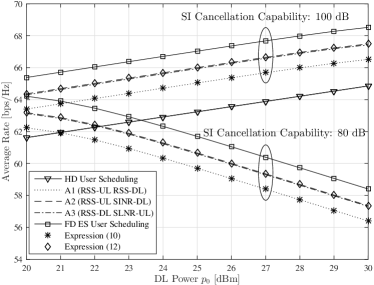
Figure 2: Average sum rate of Algorithms A1–A3 vs. the DL power $p_{0}$ for $p_{\mathcal{U}}=0.95p_{0}$ dBm and $K_{\mathcal{D}}=K_{\mathcal{U}}=5$.

In Figs. 2 and 3, the average rate of the Algorithms A1–A3 and their OPA-enhanced versions is depicted for different values of $p_{0}$ and $p_{\mathcal{U}}$, numbers of MTs in sets $\mathcal{D}$ and $\mathcal{U}$, and SI cancellation capabilities. For these results, we have used the typical values of $9$ dB noise figure for all DL MTs and $13$ dB noise figure for the small/pico cell BS, and computed $\sigma_{\mathcal{D}}^{2}$ and $\sigma_{0}^{2}$ accordingly. Therein, we also plot the rate of user scheduling in the HD mode in TDD, and that of two versions of user scheduling with exhaustive search (ES): i) the FD version that schedules concurrently one UL and one DL MT yielding the maximum FD sum rate; and ii) the FD/HD version that schedules either the MT pair of the FD version or only the best DL MT or only the best UL MT, depending on which of the latter three modes provides the maximum rate performance. Firstly, it is shown in Fig. 2 that the numerically evaluated results for (10) and (12) match perfectly with their equivalent simulations, thus validating our analysis. In both figures, we observe that A2 and A3 exhibit similar sum-rate performance, which is expectedly always superior than that of A1. This trend holds for both the original versions of the algorithms and their OPA-enhanced versions, and is mainly due to the fact that A1 ignores the inter-MT interference created after its first step. As shown in Fig. 2 for $K_{\mathcal{D}}=K_{\mathcal{U}}=5$, when the SI cancellation capability drops from $100$ to $80$ dB, increasing $p_{0}$ and $p_{\mathcal{U}}$ decreases the sum rate of the FD mode of operation. In particular, for $p_{0}\geq 23.5$ dBm and $p_{\mathcal{U}}\geq 22.3$ dBm, the performance of the optimal FD user scheduling becomes even lower than that of the HD mode. On the other hand, it is obvious from Fig. 3 that the OPA-enhanced versions of the Algorithms A1–A3 always outperform the rate of the HD user scheduling. In fact, their performance superiority over HD increases as the SI cancellation capability improves and/or the multi-user diversity increases. It was found from additional experiments not included here due to space limitation that, for SI cancellation capability equal to $80$ dB, the probability of the FD mode increases from $9\%$ to $26\%$ for $K_{\mathcal{D}}=K_{\mathcal{U}}=5$ to $K_{\mathcal{D}}=K_{\mathcal{U}}=15$. When the SI cancellation capability improves to $90$ dB, this increase is from $82\%$ for $K_{\mathcal{D}}=K_{\mathcal{U}}=5$ to $99\%$ for $K_{\mathcal{D}}=K_{\mathcal{U}}=15$. In Fig. 3, it is depicted that the performance gap between the FD/HD ES user scheduling and each of the Algorithms A1–A3 with OPA increases as $K_{\mathcal{D}}$ and $K_{\mathcal{U}}$ increase, and/or the SI cancellation capability improves, reaching a maximum value when the sum rate of the optimal FD user scheduling always outperforms the rate of the optimal HD user scheduling. For example, for SI cancellation capability equal to $110$ dB and considering the OPA-enhanced versions of A2 and A3, this gap is $0.96$ bps/Hz for $K_{\mathcal{D}}=K_{\mathcal{U}}=5$ and $2.16$ bps/Hz for $K_{\mathcal{D}}=K_{\mathcal{U}}=15$.

Finally, in Fig. 4, we plot the sum rate of the proposed algorithms with and without the OPA enhancement versus the number of DL MTs $K_{\mathcal{D}}$ ($K_{\mathcal{D}}=K_{\mathcal{U}}$). The performance of the OPA-enhanced algorithms is very close to the optimal ES for both considered values of the signal-to-noise ratio (SNR), while the performance gap of user scheduling without OPA decreases for increasing $K_{\mathcal{D}}$. This implies that, with a large number of MTs to select from, the FD mode outperforms the HD one. Otherwise stated, multi-user diversity can compensate for the SI and the inter-MT interference due to the FD operation and boost the FD sum-rate performance.

Figure 3: Average rate of Algorithms A1–A3 with OPA vs. the SI cancellation capability for $p_{0}=24$ dBm and $p_{\mathcal{U}}=23$ dBm.

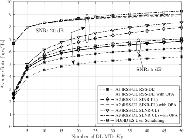
Figure 4: Average rate of Algorithms A1–A3 and their OPA enhancements vs. the number of DL MTs $K_{\mathcal{D}}$ for $K_{\mathcal{U}}=K_{\mathcal{D}}$ and SI cancellation capability of $20$ dB.

VI Conclusion

In this paper, we investigated the problem of user scheduling and power control in FD cellular systems. We proposed three low complexity user scheduling algorithms to maximize the sum rate. We also derived the optimal power allocation for the two communication links and introduced efficient metrics for FD/HD mode switching as a means to further increase the system rate performance. For two of the proposed user scheduling algorithms for FD communication we presented closed-form expressions for their average sum-rate performance over Rayleigh fading. Our performance evaluation results unveiled that power control and low complexity user scheduling can boost the performance of FD small/pico cells.

Appendix A Proof of Theorem 1

The instantaneous sum rate of the considered FD system can be rewritten as $\mathsf{R}(p_{0},p_{\mathcal{U}})=\log_{2}\left(1+\varphi(p_{0},p_{\mathcal{U}})\right)$, where we have defined the following real positive function for $x,y\geq 0$:

$$\varphi(x,y)\triangleq\ \frac{x|h_{d^{\star},0}|^{2}}{y|h_{d^{\star},u^{\star}}|^{2}+\sigma_{d^{\star}}^{2}}+\frac{y|h_{0,u^{\star}}|^{2}}{x|h_{0,0}|^{2}+\sigma_{0}^{2}}$$ (I.1)

$$+\frac{xy|h_{d^{\star},0}|^{2}|h_{0,u^{\star}}|^{2}}{\big{(}y|h_{d^{\star},u^{\star}}|^{2}+\sigma_{d^{\star}}^{2}\big{)}\big{(}x|h_{0,0}|^{2}+\sigma_{0}^{2}\big{)}}.$$

Recall the definitions of $\zeta(p_{\mathcal{U}})$ and $\eta(p_{0})$ in (6) and in (7), respectively. From $\frac{\partial\varphi(p_{0},p_{\mathcal{U}})}{\partial p_{\mathcal{U}}}$ and $\frac{\partial^{2}\varphi(p_{0},p_{\mathcal{U}})}{\partial p_{\mathcal{U}}^{2}}$, it is straightforward to show that:

• If $\zeta(p_{\mathcal{U}})\geq 0$, then $\varphi(p_{0},p_{\mathcal{U}})$ is strictly increasing and concave in $p_{0}$ and $\operatornamewithlimits{argmax}_{p_{0}\in[0,P_{0}]}\mathsf{R}(p_{0},p_{\mathcal{U}})=P_{0}$;

• If $\zeta(p_{\mathcal{U}})<0$, then $\varphi(p_{0},p_{\mathcal{U}})$ is strictly convex in $p_{0}$ and $\operatornamewithlimits{argmax}_{p_{0}\in[0,P_{0}]}\mathsf{R}(p_{0},p_{\mathcal{U}})\in\{0,P_{0}\}$.

Likewise, from $\frac{\partial\varphi(p_{0},p_{\mathcal{U}})}{\partial p_{\mathcal{U}}}$ and $\frac{\partial^{2}\varphi(p_{0},p_{\mathcal{U}})}{\partial p_{\mathcal{U}}^{2}}$, it is not difficult to conclude that:

• If $\eta(p_{0})\geq 0$, then $\varphi(p_{0},p_{\mathcal{U}})$ is strictly increasing and concave in $p_{\mathcal{U}}$ and $\operatornamewithlimits{argmax}_{p_{\mathcal{U}}\in[0,P_{\mathcal{U}}]}\mathsf{R}(p_{0},p_{\mathcal{U}})=P_{\mathcal{U}}$;

• If $\eta(p_{0})<0$, then $\varphi(p_{0},p_{\mathcal{U}})$ is strictly convex in $p_{\mathcal{U}}$ and $\operatornamewithlimits{argmax}_{p_{\mathcal{U}}\in[0,P_{\mathcal{U}}]}\mathsf{R}(p_{0},p_{\mathcal{U}})\in\{0,P_{\mathcal{U}}\}$.

Putting all above together, we have shown that $p_{0}^{\star}\in\{0,P_{0}\}$ and $p_{\mathcal{U}}^{\star}\in\{0,P_{\mathcal{U}}\}$. Hence, one can check directly the conditions on $\eta(P_{0})$ and $\zeta(P_{\mathcal{U}})$, as stated in Theorem 1, to determine the OPA strategy. This completes the proof.

Appendix B Proof of Theorem 2

Starting from the DL communication, the CDF of the DL SINR $\gamma_{d^{\star}}$ in (4) for the Algorithm A1 can be obtained as

$$F_{\gamma_{d^{\star}}}(x) =\hskip 2.27621pt\mathbb{P}\left[|h_{d^{\star},0}|^{2}<\frac{p_{\mathcal{U}}|h_{d^{\star},u^{\star}}|^{2}+\sigma_{\mathcal{D}}^{2}}{p_{0}}x\right]$$ (II.1)

$$\stackrel{{\scriptstyle(\rm{a})}}{{=}}\int_{0}^{\infty}\mathbb{P}\left[\kappa<\frac{p_{\mathcal{U}}y+\sigma_{\mathcal{D}}^{2}}{p_{0}}x\bigg{|}y\right]f_{\lambda}(y)\mathrm{d}y$$

$$\stackrel{{\scriptstyle(\rm{b})}}{{=}}\int_{0}^{\infty}\left(1-\exp\left(-\frac{p_{\mathcal{U}}y+\sigma_{\mathcal{D}}^{2}}{p_{0}}x\right)\right)^{K_{\mathcal{D}}}\!f_{\lambda}(y)\mathrm{d}y,$$

where in $(\rm{a})$ we condition on $\lambda\triangleq|h_{d^{\star},u^{\star}}|^{2}$ and we use the fact that $\lambda$ and $\kappa\triangleq\max_{d\in\mathcal{D}}|h_{d,0}|^{2}$ are independent, and in $(\rm{b})$ we use the CDF of the maximum of $K_{\mathcal{D}}$ independent and identically distributed (i.i.d.) exponential RVs. By applying the binomial expansion and using [9, Eq. (3.381/4)] to solve the resulting integrals, $F_{\gamma_{d^{\star}}}(x)$ can be derived in closed form as

$$F_{\gamma_{d^{\star}}}(x)=\sum_{k=0}^{K_{\mathcal{D}}}\binom{K_{\mathcal{D}}}{k}\!\left(-1\right)^{k}\!\left(k\frac{p_{\mathcal{U}}}{p_{0}}x+1\right)^{-1}\!\!\exp\left(\!-k\frac{\sigma_{\mathcal{D}}^{2}}{p_{0}}x\right).$$ (II.2)

The CDF of the UL SINR $\gamma_{0}$ in (3) for the Algorithm A1 (using the UL MT selection criterion in ($\mathrm{A1.1}$)) can be derived in a similar way to (II.1), and results in

$$F_{\gamma_{0}}(x) =\mathbb{P}\left[\max_{u\in\mathcal{U}}|h_{0,u}|^{2}<\frac{p_{0}|h_{0,0}|^{2}+\sigma_{0}^{2}}{p_{\mathcal{U}}}x\right]$$ (II.3)

$$=\sum_{k=0}^{K_{\mathcal{U}}}\binom{K_{\mathcal{U}}}{k}\left(-1\right)^{k}\exp\left(-\frac{p_{0}|h_{0,0}|^{2}+\sigma_{0}^{2}}{p_{\mathcal{U}}}kx\right).$$

By substituting (II.1) and (II.3) into (8), and then applying the integration theory of rational functions [9, Sec. 2.102] and using [9, Eq. (3.352/4)], the average sum rate with the Algorithm A1 is obtained as in (10) after some algebraic manipulations.

Appendix C Proof of Theorem 3

The selection criterion of the UL MT with the Algorithm A2 is the same as with the Algorithm A1 and, hence, we have the same average rate for the UL communication (cf. expression (11)). Focusing then on the DL communication, the CDF of DL SINR $\gamma_{d^{\star}}$ in (4) for the Algorithm A2 (using the DL MT selection criterion in ($\mathrm{A2.1}$)) can be obtained as

$$F_{\gamma_{d^{\star}}}(x) =\mathbb{P}\left[\max_{d\in\mathcal{D}}\frac{p_{0}|h_{d,0}|^{2}}{p_{\mathcal{U}}|h_{d,u^{\star}}|^{2}+\sigma_{\mathcal{D}}^{2}}<x\right]$$ (III.1)

$$\stackrel{{\scriptstyle(\rm{c})}}{{=}}\left(\int_{0}^{\infty}\mathbb{P}\left[\tau<\frac{p_{\mathcal{U}}y+\sigma_{\mathcal{D}}^{2}}{p_{0}}x\bigg{|}y\right]f_{\nu}(y)\mathrm{d}y\right)^{K_{\mathcal{D}}}$$

$$\stackrel{{\scriptstyle(\rm{d})}}{{=}}\sum_{k=0}^{K_{\mathcal{D}}}\binom{K_{\mathcal{D}}}{k}\left(-\frac{p_{\mathcal{U}}}{p_{0}}x-1\right)^{-k}\exp\left(-\frac{\sigma_{\mathcal{D}}^{2}}{p_{0}}kx\right),$$

where in $(\rm{c})$ we condition on $\nu\triangleq|h_{d,u^{\star}}|^{2}$ and use the fact that $\nu$ and $\tau\triangleq|h_{d,0}|^{2}$ are stochastically independent (for the proposed decoupled UL/DL user scheduling), and $(\rm{d})$ follows after substituting the marginal PDF of an exponential RV, then using [9, Eq. (3.381/4)], and finally applying the binomial expansion. By substituting (III.1) and (II.3) into (8), and then applying [9, Sec. 2.102] and using [9, Eq. (3.353/2)], the average sum rate with the Algorithm A2 is obtained as in (12) after some algebraic manipulations.

Appendix D Proof of Theorem 4

The scaling result in (13) for the sum rate with the Algorithm A1 is based on the following lemma for the Jensen’s inequality for the logarithmic function.

Lemma 1.

Let $\mathcal{I}\triangleq\{1,2,\ldots,K\}$ and $Y_{i}$ $\forall i\!\in\!\mathcal{I}$ be a sequence of positive i.i.d. RVs. Also, let $Z_{K}\triangleq\max_{i\in\mathcal{I}}Y_{i}$ with finite mean $\mu_{K}$ and finite variance $\sigma_{K}^{2}$, and $\mathbb{E}\left[\log(Z_{K})\right]<\infty$. If $\displaystyle\lim_{K\rightarrow\infty}\!\!\sigma_{K}^{2}\mu_{K}^{-1}\!\to\!0$, then $\log\mu_{K}-\mathbb{E}[\log Z_{K}]\!\rightarrow\!0$ as $K\!\rightarrow\!\infty$.

Since $|h_{0,u}|^{2}$ $\forall u\!\in\!\mathcal{U}$ are i.i.d. exponential RVs, the mean and variance of the RV $Z_{K_{\mathcal{U}}}\triangleq\max_{u\in\mathcal{U}}|h_{0,u}|^{2}$ for $K_{\mathcal{U}}\to\infty$ are given by $\mu_{K_{\mathcal{U}}}=\mathcal{H}_{K_{\mathcal{U}}}\sim\log(K_{\mathcal{U}})+\gamma$ and $\sigma^{2}_{K_{\mathcal{U}}}\sim\pi^{2}/6$, respectively, where $\mathcal{H}_{K_{\mathcal{U}}}$ is the $K_{\mathcal{U}}$-th harmonic number and $\gamma\cong 0.577$ is the Euler-Mascheroni constant [10]. Hence, we have that $\displaystyle\lim_{K_{\mathcal{U}}\rightarrow\infty}\!\!\sigma_{K_{\mathcal{U}}}^{2}\mu_{K_{\mathcal{U}}}^{-1}\!\to\!0$; therefore, it holds for $\overline{\mathsf{R}}_{0}$ that

$$\overline{\mathsf{R}}_{0}\approx\log(\log(K_{\mathcal{U}}))+\log\left(\frac{p_{\mathcal{U}}}{p_{0}|h_{0,0}|^{2}+\sigma_{0}^{2}}\right).$$ (IV.1)

Using similar tools from the extreme value theory, we can show that $\overline{\mathsf{R}}_{d^{\star}}\approx\log(\log(K_{\mathcal{D}}))$, which concludes the proof.

References

• [1] M. Duarte, C. Dick, and A. Sabharwal, “Experiment-driven characterization of full-duplex wireless systems,” IEEE Trans. Wireless Commun., vol. 11, no. 12, pp. 4296–4307, Dec. 2012.
• [2] S. Goyal, P. Liu, S. S. Panwar, R. A. Difazio, R. Yang, and E. Bala, “Full duplex cellular systems: Will doubling interference prevent doubling capacity?” IEEE Commun. Mag., vol. 53, no. 5, pp. 121–127, May 2015.
• [3] Y. Wang and S. Mao, “Distributed power control in full duplex wireless networks,” in Proc. IEEE WCNC, New Orleans, USA, 9–12 Mar. 2015, pp. 1165–1170.
• [4] W. Cheng, X. Zhang, and H. Zhang, “Optimal dynamic power control for full-duplex bidirectional-channel based wireless networks,” in Proc. IEEE INFOCOM, Turin, Italy, 14–19 Apr. 2013, pp. 3120–3128.
• [5] R. Sultan, L. Song, K. G. Seddik, Y. Li, and Z. Han, “Mode selection, user pairing, subcarrier allocation and power control in full-duplex OFDMA HetNets,” in Proc. IEEE ICC, London, UK, 8–12 June 2015, pp. 210–215.
• [6] H. H. Choi, “On the design of user pairing algorithms in full duplexing wireless cellular networks,” in Proc. IEEE ICTC, Busan, South Korea, 22–24 Oct. 2014, pp. 490–495.
• [7] A. Gjendemsjø, D. Gesbert, G. E. Øien, and S. G. Kiani, “Binary power control for sum rate maximization over multiple interfering links,” IEEE Trans. Wireless Commun., vol. 7, no. 8, pp. 3164–3173, Aug. 2008.
• [8] I. Atzeni and M. Kountouris, “Full-duplex MIMO small-cell networks: Performance analysis,” in Proc. IEEE GLOBECOM, San Diego, USA, 6–10 Dec. 2015, pp. 1–6.
• [9] I. S. Gradshteyn and I. M. Ryzhik, Table of Integrals, Series, and Products, 7th ed.   New York, NY, USA: Academic Press, 2007.
• [10] L. de Haan and A. Ferreira, Extreme Value Theory.   NY, USA: Springer, 2006.
• [11] I. Atzeni, M. Kountouris, and G. C. Alexandropoulos, “Performance evaluation of user scheduling for full-duplex small cells in ultra-dense networks,” in Proc. EW Conf., Oulu, Finland, 18–20 May 2016, pp. 1–6.