A NLTE line formation for neutral and singly-ionised titanium in model atmospheres of the reference A-K stars
Abstract
We construct a model atom for Ti i– ii using more than 3600 measured and predicted energy levels of Ti i and 1800 energy levels of Ti ii, and quantum mechanical photoionisation cross-sections. Non-local thermodynamical equilibrium (NLTE) line formation for Ti i and Ti ii is treated through a wide range of spectral types from A to K, including metal-poor stars with [Fe/H] down to dex. NLTE leads to weakened Ti i lines and positive abundance corrections. The magnitude of NLTE corrections is smaller compared to the literature data for FGK atmospheres. NLTE leads to strengthened Ti ii lines and negative NLTE abundance corrections. For the first time, we performed the NLTE calculations for Ti i– ii in the 6500 K 13000 K range. For four A type stars we derived in LTE an abundance discrepancy of up to 0.22 dex was obtained between Ti i and Ti ii and it vanishes in NLTE. For other four A-B stars, with only Ti ii lines observed, NLTE leads to decrease of line-to-line scatter. An efficiency of inelastic Ti i + H i collisions was estimated from analysis of Ti i and Ti ii lines in 17 cool stars with [Fe/H] 0.0. Consistent NLTE abundances from Ti i and Ti ii were obtained applying classical Drawinian rates for the stars with log 4.1, and neglecting inelastic collisions with H i for the VMP giant HD 122563. For the VMP turn-off stars ([Fe/H] and log 4.1), we obtained the positive abundance difference Ti i– ii already in LTE and it increases in NLTE. The accurate collisional data for Ti i and Ti ii are desired to find a clue to this problem.
keywords:
line: formation – stars: atmospheres – stars: fundamental parameters – stars: abundances.1 Introduction
Titanium is observed in lines of two ionisation stages, Ti i and Ti ii, in a wide range of spectral types from A to K. Experimental oscillator strengths () for Ti i and Ti ii were measured using a common method (Lawler et al., 2013; Wood et al., 2013, respectively), which permits to use Ti i and Ti ii lines for determination of accurate titanium abundances and stellar atmosphere parameters. Bergemann (2011) and Bergemann et al. (2012) investigated the non-local thermodynamic equilibrium (NLTE) line-formation for Ti i- ii in the atmospheres of cool stars. The first paper presents the NLTE calculations for the Sun and four metal-poor stars with 6350 K while the second one for red supergiants with 3400 K 4400 K, log 1.0, and [Fe/H] 0.5. Bergemann (2011) found that the deviations from LTE are small in the solar atmosphere, with the abundance difference between NLTE and LTE (the NLTE abundance correction, ) not exceeding 0.11 dex for Ti i lines. For the Sun Bergemann (2011) derived consistent within 0.04 dex NLTE abundances from Ti i and Ti ii lines. However, she failed to achieve the Ti i/Ti ii ionisation equilibrium for cool metal-poor (MP, [Fe/H] ) dwarfs with well-determined atmospheric parameters. Bergemann (2011) suggested that this can be caused by: (i) neglecting high-excitation levels of Ti i in the used model atom; (ii) using hydrogenic photoionisation cross-sections; (iii) using a rough theoretical approximation (Drawin, 1968, 1969) for inelastic collisions with hydrogen atoms. We eliminate the first two points in this study. We still rely on the Drawinian approximation because accurate laboratory measurements or quantum mechanical calculations for inelastic Ti i H i collisions are not available. Poorly-known collisions with H i atoms is the main source of the uncertainties in the NLTE results for stars with 7000 K.
For the atmospheres hotter than 6500 K the NLTE calculations for Ti i– ii were not yet performed, although the observations indicate a discrepancy in LTE abundances between Ti i and Ti ii. For example, Bikmaev et al. (2002) derived under the LTE assumption the abundance difference Ti i–Ti ii111Here, log A(X)=log(), where Ntot is a total number density; X i–X ii means difference in abundance derived from lines of X i and X ii, log A(X i)–log A(X ii). = dex and dex for the A-type stars HD 32115 and HD 37954, respectively. Becker (1998) performed the NLTE calculations for Ti ii in A-type stars (Vega, supergiants Leo and 41-3712 from M31) and found that NLTE leads to weakened Ti ii lines, with the NLTE abundance corrections being larger for weak lines compared with those calculated for strong lines. Using model atom from Becker (1998), Przybilla et al. (2006) and Schiller & Przybilla (2008) derived the NLTE abundances from lines of Ti ii in BA-type supergiants and concluded that proper NLTE calculations reduce the line-to-line scatter.
We aim to construct a comprehensive model atom of Ti i– ii and to treat a reliable method of abundance determination from different lines of Ti i and Ti ii in a wide range of stellar spectral types from late B to K, including metal-poor stars. First, we test the new model atom employing the stars with 7100 K, where inelastic collisions with hydrogen atoms do not affect the statistical equilibrium (SE). Then, we empirically constrain an efficiency of collisions with H i from analysis of Ti i and Ti ii lines in spectra of cool metal-poor stars. In total, we analyse titanium lines in 25 well-studied stars.
We present the constructed model atom and the NLTE mechanism for Ti i and Ti ii in Section 2. Section 3 describes observations and stellar parameters of our stellar sample. The obtained results for hot and cool stars are considered in Sections 4 and 5, respectively. Our conclusions and recommendations are given in Sect. 6.
2 Method of NLTE calculations for Ti i– ii
In this section we describe the model atom of titanium, the programs used for computing the level populations and spectral line profiles, and mechanisms of departures from LTE for Ti i and Ti ii.
2.1 The model atom
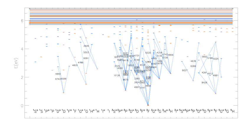
Energy levels. Titanium is almost completely ionised throughout the atmosphere of stars with effective temperatures above 4500 K. For example, the ratio throughout the solar atmosphere. Such minority species as Ti i are particularly sensitive to NLTE effects because any small deviation in the intensity of ionising radiation from the Plank function strongly changes their population. For accurate calculations of the SE we include in our model atom high-excitation levels of Ti i and Ti ii, which establish collisional coupling of Ti i and Ti ii levels near the continuum to the ground states of Ti ii and Ti iii, respectively. Mashonkina et al. (2011) included high-excitation levels of Fe i in their Fe i– ii model atom, and found that the SE of iron changed substantially by achieving close collisional coupling of the Fe i levels near the continuum to the ground state of Fe ii. Our model atom of titanium (Fig. 1, 2) is constructed using not only all the known energy levels from NIST (Ralchenko et al., 2008), but also the predicted levels from atomic structure calculation of R. Kurucz (). The measured levels of Ti i with the excitation energy 6 eV belong to 175 terms. Neglecting their fine structure, except for the ground state of Ti i, we obtain 177 levels in the model atom. The predicted and measured levels below the threshold, in total 3500 ones with 6 eV, with common parity and close energies were combined whenever the energy separation is smaller than = 0.1 eV. This makes up 17 super-levels.
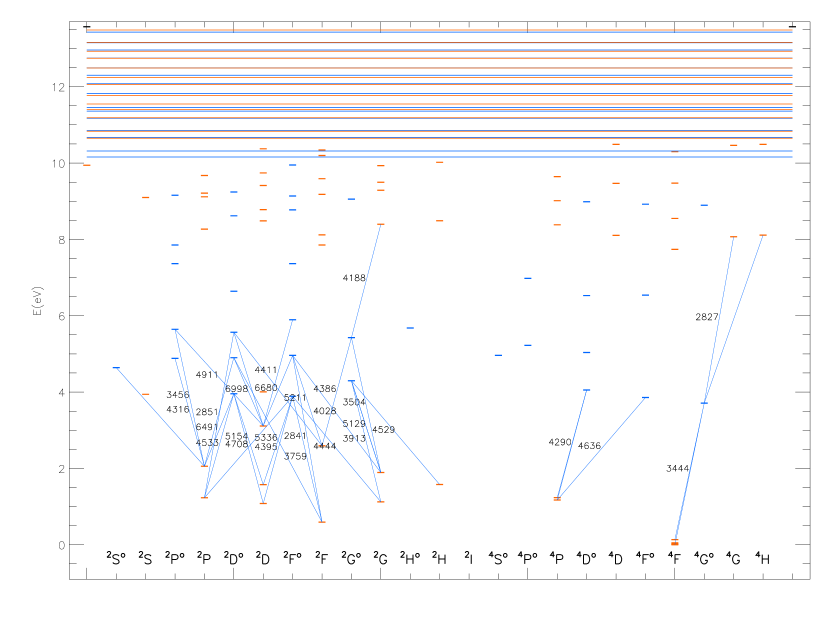
For Ti ii we use the experimental energy levels belonging to 89 terms with up to 10.5 eV. The fine structure is neglected, except for the ground state of Ti ii. The 1800 high excitation levels with eV are used to make up 28 super-levels. The ground state of Ti iii completes the system of levels in the model atom.
Radiative bound-bound (b-b) transitions. In total, 7929 and 3104 allowed transitions of Ti i and Ti ii, respectively, occur in our final model atom. Their average f-values are calculated using the data from R. Kurucz database. We compared predicted gf-values with accurate laboratory data for about 900 transitions of Ti i (Lawler et al., 2013) and found a systematic shift to be minor, with an average difference of log gflab – log gfKurucz = 0.28. An advantage of the Kurucz’s predicted gf-values is their completeness that is of extreme importance for the statistical equilibrium calculations. For the transitions involving the superlevels the total gf-value was calculated as a sum of gf of individual transitions , i = 1,…, Nl, j = 1,…, Nu, where Nl and Nu are numbers of individual levels, which form a lower and upper superlevel, respectively. Radiative rates were computed using the Voigt profiles for transitions with and 1800 Å 4000 Å and the Doppler profiles for the remaining ones. The transitions with were treated as forbidden ones.
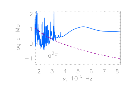
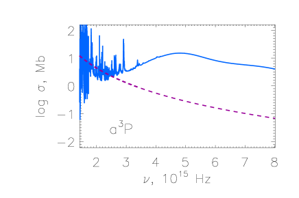
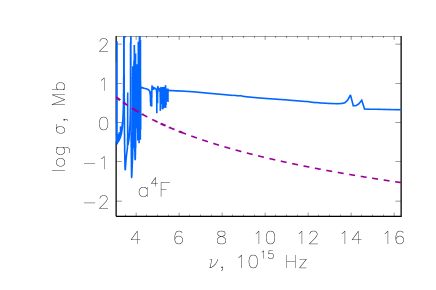
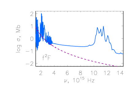
Radiative bound-free (b-f) transitions. For 115 terms of Ti i with 5.5 eV we use photoionisation cross-sections from calculations of Nahar (2015), based on the close-coupling R-matrix method, and for 78 terms of Ti ii with 10.0 eV we use the data from quantum-mechanical calculations of Keith Butler (private communication). For the remaining high-excitation levels we assume a hydrogenic approximation with using an effective principle quantum number. We compare the quantum-mechanical photoionisation cross-sections with the hydrogenic ones for selected levels of Ti i and Ti ii in Fig. 3 and 4, respectively. For each level the hydrogenic cross-sections fit, on average, the quantum-mechanical ones near the ionisation threshold. The difference at frequencies higher than 3.29 Hz ( 912 Å) weakly affects the photoionisation rate because of small flux in this spectral range in the investigated stellar atmospheres.
Collisional transitions. All levels in our model atom are coupled via collisional excitation and ionisation by electrons and by neutral hydrogen atoms. Our calculations of collisional rates rely on the theoretical approximations because no accurate experimental or theoretical data are available. For electron-impact excitation we use the formula of van Regemorter (1962) for the allowed transitions and the formula from Woolley & Allen (1948) with a collision strength of 1.0 for the radiatively forbidden transitions. Ionisation by electronic collisions is calculated from the Seaton (1962) approximation using the threshold photoionisation cross-section.
For collisions with H i atoms, we employ the formula of Steenbock & Holweger (1984) based on theory of Drawin (1968, 1969) for allowed b-b and b-f transitions and, following Takeda (1994), a simple relation between hydrogen and electron collisional rates, C, for forbidden transitions. Due to the Drawin formula provides order-of-magnitude estimates, we perform the NLTE calculations using a scaling factor =0.1, 0.5 and 1, and constrain its magnitude empirically from analysis of metal-poor stars.
The nearly resonance charge exchange reaction (CER) H+ + Ti ii H i + Ti iii takes place because the ionisation thresholds for Ti ii and H i are 13.57 eV and 13.60 eV, respectively. There are no literature data on cross-sections for this process. In order to inspect an influence of CER on the statistical equilibrium of titanium, we assumed that the analytic fit deduced by Arnaud & Rothenflug (1985) for O i can also be applied to Ti ii, because the ionisation threshold for O i is close to that for Ti ii and amounts to 13.62 eV. Test calculations for A-type stars showed that the CER makes the populations of the ground states of Ti iii and Ti ii to be in thermodynamic equilibrium, nevertheless, no change in the NLTE abundances from lines of Ti ii was found. For stars with 9000 K the CER weakly affects the SE because of small fraction of Ti iii.
2.2 Programs and model atmospheres
The coupled radiative transfer and SE equations were solved with a revised version of the detail code by Butler & Giddings (1985). The opacity package of the detail code was updated as described by Przybilla et al. (2011) and Mashonkina et al. (2011), by including the quasi-molecular Lyα satellites following the implementation by Castelli & Kurucz (2001) of the Allard et al. (1998) theory and using the Opacity Project (see Seaton et al., 1994, for a general review) photoionisation cross-sections for the calculations of b-f absorption of C i, N i, O i, Mg i, Si i, Al i, Ca i, and Fe i. In addition to the continuous background opacity, the line opacity introduced by H i and metal lines was taken into account by explicitly including it in solving the radiation transfer. The metal line list was extracted from the Kurucz (1994) compilation and the VALD database (Kupka et al., 1999). The pre-calculated departure coefficients were then used by synthV_NLTE code updated in Ryabchikova et al. (2016), and based on Tsymbal (1996) to compute the theoretical synthetic spectra. The integration of the synthV_NLTE code in the idl binmag3 code by O. Kochukhov222http://www.astro.uu.se/oleg/download.html allows us to obtain the best fit to the observed line profiles with the NLTE effects taken into account.
Throughout this study, the element abundance is determined from line profile fitting. For late type stars we used classical plane-parallel model atmospheres from the marcs model grid (Gustafsson et al., 2008), which were interpolated for given , log , and [Fe/H] using a FORTRAN-based routine written by Thomas Masseron333http://marcs.astro.uu.se/software.php. For A-B type stars the model atmospheres were calculated under the LTE assumption with the code LLmodels (Shulyak et al., 2004).
For each star the line list includes unblended lines of various strength ( 150 mÅ, where is the line equivalent width) and excitation energies. The full list of the lines is presented in Table 1 along with the transition information, gf-value, excitation energy, and damping constants (log , log , log at 10000 K). The line list was extracted from the VALD database (Kupka et al., 1999; Ryabchikova et al., 2015). The adopted oscillator strengths for most lines of both ions were measured by a common method (Lawler et al., 2013; Wood et al., 2013, – Wisconsin data), and, hence, represent homogeneous set of gf-values.
| , Å | , eV | log gf | transition | log | log | log |
|---|---|---|---|---|---|---|
| Ti i | ||||||
| 4008.927 | 0.021 | -1.000 | 3a3F – y3F | 8.000 | -6.080 | -7.750 |
| 4060.262 | 1.052 | -0.690 | a3P – x3P | 8.050 | -6.050 | -7.646 |
| 4287.403 | 0.836 | -0.370 | a5F – x5D | 8.230 | -6.010 | -7.570 |
| 4449.143 | 1.886 | 0.470 | a3G – v3G | 8.120 | -5.560 | -7.579 |
| 4453.699 | 1.872 | 0.100 | a3G – v3G | 8.110 | -4.970 | -7.582 |
| 4512.733 | 0.836 | -0.400 | a5F – y5F | 8.130 | -5.120 | -7.593 |
| 4533.240 | 0.848 | 0.540 | a5F – y5F | 8.130 | -5.120 | -7.593 |
| 4534.776 | 0.836 | 0.350 | a5F – y5F | 8.130 | -5.280 | -7.596 |
| 4548.763 | 0.826 | -0.280 | a5F – y5F | 8.130 | -5.410 | -7.598 |
| 4555.484 | 0.848 | -0.400 | a5F – y5F | 8.130 | -5.280 | -7.596 |
| … | ||||||
2.3 Statistical equilibrium of Ti i- ii
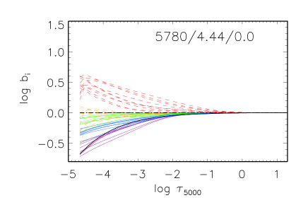
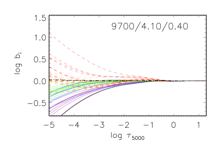
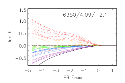
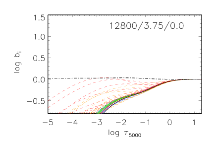
In this section, we consider the NLTE effects for Ti i– ii in various model atmospheres. The deviations from LTE in level populations are characterized by the departure coefficients bi = n/n, where n and n are the statistical equilibrium and thermal (Saha-Boltzmann) number densities, respectively. The departure coefficients for the selected levels of Ti i, Ti ii and the ground state of Ti iii in the model atmospheres 5777/4.44/0, 6350/4.09/, 9700/4.1/0.4 and 12800/3.75/0 are presented in Fig. 5. All the levels retain their LTE populations in deep atmospheric layers below log = 0. In the higher atmospheric layers a total number density of Ti i is lower compared with the TE value. The overionisation is caused by superthermal radiation of non-local origin below the thresholds of the low excitation levels of Ti i. In the atmospheres, where Ti ii is the majority species, collisional recombinations to the Ti i high-excitation levels followed by cascades of spontaneous transitions tend to compensate a depopulation of the lower levels of Ti i. However, this process can not prevent the overionisation. High superlevels of Ti i are collisionally coupled to the ground state of Ti ii. NLTE leads to weakened lines of Ti i compared to their LTE strengths.
High levels of Ti ii are overpopulated via radiative pumping transitions from the low excitation levels. The NLTE effects for Ti ii are small in cool atmospheres. In the models 5780/4.44/0.0 and 6350/4.09/ a behaviour of the departure coefficients is qualitatively similar. However a magnitude of the NLTE effects grows towards higher and lower log and [Fe/H]. In the models representing atmospheres of A-type stars high levels of Ti ii retain their LTE populations inward log = , and become underpopulated in the higher atmospheric layers. This results in strengthening the Ti ii line cores formed in the uppermost layers compared with LTE. In the hottest model atmosphere 12800/3.75/0.0 Ti iii becomes the majority species, while the levels of Ti ii are underpopulated beginning at log 0.5. Overionisation of Ti ii results in weakened Ti ii lines.
3 Observations and stellar atmosphere parameters
Our sample includes the Sun and 24 well-studied stars. They are listed in Table 2. Atmospheric parameters (, log , [Fe/H], ) were either determined in our earlier studies or taken from the literature. These parameters were derived by several independent methods, which gave consistent results. Our hot stellar sample consists of A and late B stars, which do not reveal pulsation activity, chemical stratification and magnetic field. For Sirius, Cet, 21 Peg, HD 32115, HD 37594, HD 73666, HD 145788 atmospheric parameters were derived by common method, based on multicolour photometry, analysis of hydrogen Balmer lines and metal lines in high resolution spectra and comparison of spectrophotometric data with theoretical flux (see Table 2 for the references). For HD 72660 the parameters 9700/4.10/0.45/1.8 were derived by fitting the 4400-5200 Å and 6400-6700 Å spectral regions with sme (Spectroscopy Made Easy) program package (Valenti & Piskunov, 1996). We used medium-resolution spectrum of HD 72660 extracted from ELODIE archive111http://atlas.obs-hp.fr/elodie/. sme was tested for Sirius, Cet, 21 Peg, and HD 32115 by Ryabchikova et al. (2015) where the authors derived practically the same parameters as adopted in the present paper. Atmospheric parameters of HD 72660 agree with the results of Lemke (1989), who derived /log = 9770/4.0 from photometry and Hβ, and Landstreet et al. (2009), who derived 9650/4.05.
Each cool star of the sample has photometric and log based on the Hipparcos parallax. We checked in advance whether an ionisation equilibrium between Fe i and Fe ii is fulfilled in NLTE when using non-spectroscopic parameters. The iron abundances obtained from the lines of Fe i and Fe ii in dwarfs agree within 0.05 dex in NLTE, when using = 0.5 (Sitnova et al., 2015). To confirm the adopted parameters, we checked them with evolutionary tracks and derived reasonable masses and ages. Our sample also includes the most metal-poor giant, HD 122563 ([Fe/H] = ), with the accurate Hipparcos parallax available. The effective temperature of HD 122563 was determined by Creevey et al. (2012) based on angular diameter measurements.
| Star | , | [Fe/H] | , | Ref. | , | source | ||
| K | km s-1 | 103 | ||||||
| Sun | 5777 | 4.44 | 0.0 | 0.9 | – | 300 | 300 | KPNO84 |
| HD 24289 | 5980 | 3.71 | –1.94 | 1.1 | S15 | 60 | 110 | S15 |
| HD 64090 | 5400 | 4.70 | –1.73 | 0.7 | S15 | 60 | 280 | S15 |
| HD 74000 | 6225 | 4.13 | –1.97 | 1.3 | S15 | 60 | 140 | S15 |
| HD 84937 | 6350 | 4.09 | –2.16 | 1.7 | S15 | 80 | 200 | UVESPOP1 |
| HD 94028 | 5970 | 4.33 | –1.47 | 1.3 | S15 | 60 | 120 | S15 |
| HD 103095 | 5130 | 4.66 | –1.26 | 0.9 | S15 | 60 | 200 | FOCES2 |
| HD 108177 | 6100 | 4.22 | –1.67 | 1.1 | S15 | 60 | 60 | S15 |
| HD 140283 | 5780 | 3.70 | –2.46 | 1.6 | S15 | 80 | 200 | UVESPOP |
| BD–4∘ 3208 | 6390 | 4.08 | –2.20 | 1.4 | S15 | 80 | 200 | UVESPOP |
| BD–13∘ 3442 | 6400 | 3.95 | –2.62 | 1.4 | S15 | 60 | 100 | S15 |
| BD+7∘ 4841 | 6130 | 4.15 | –1.46 | 1.3 | S15 | 120 | 150 | S15 |
| BD+9∘ 0352 | 6150 | 4.25 | –2.09 | 1.3 | S15 | 120 | 160 | S15 |
| BD+24∘ 1676 | 6210 | 3.90 | –2.44 | 1.5 | S15 | 60 | 90 | S15 |
| BD+29∘ 2091 | 5860 | 4.67 | –1.91 | 0.8 | S15 | 60 | 80 | S15 |
| BD+66∘ 0268 | 5300 | 4.72 | –2.06 | 0.6 | S15 | 60 | 110 | S15 |
| G 090–003 | 6010 | 3.90 | –2.04 | 1.3 | S15 | 60 | 100 | S15 |
| HD 122563 | 4600 | 1.60 | –2.60 | 2.0 | M11 | 80 | 200 | UVESPOP |
| HD 32115 | 7250 | 4.20 | 0.0 | 2.3 | F11 | 60 | 490 | F11 |
| HD 37594 | 7150 | 4.20 | -0.30 | 2.5 | F11 | 60 | 535 | F11 |
| HD 72660 | 9700 | 4.10 | 0.45 | 1.8 | this study | 30 | 150 | STIS3, L98 |
| HD 73666 | 9380 | 3.78 | 0.10 | 1.8 | F07, F10 | 65 | 660 | F07 |
| HD 145788 | 9750 | 3.70 | 0.0 | 1.3 | F09 | 115 | 200 | F09 |
| HD 209459 | 10400 | 3.55 | 0.0 | 0.5 | F09 | 120 | 700 | F09 |
| (21 Peg) | ||||||||
| HD 48915 | 9850 | 4.30 | 0.4 | 1.84 | H93 | 70 | 500 | F95 |
| (Sirius) | ||||||||
| HD 17081 | 12800 | 3.75 | 0.0 | 1.0 | F09 | 65 | 200 | F09 |
| ( Cet) | ||||||||
| 1 Bagnulo et al. (2003), 2 K. Fuhrmann, private communication, 3 J. Landstreet, private communication, 4 Sitnova et al. (2013), KPNO84 = Kurucz et al. (1984), S15 = Sitnova et al. (2015), M11 = Mashonkina et al. (2011), H93 = Hill & Landstreet (1993), F95 = Furenlid et al. (1995), F07 = Fossati et al. (2007), F09 = Fossati et al. (2009), F10 = Fossati et al. (2010), F11 = Fossati et al. (2011), L98 = Landstreet (1998). | ||||||||
4 Analysis of Ti i and Ti ii lines in A-B-type stars
A-B type stars are suitable for testing the treated model atom because the deviations from LTE are large for both Ti i and Ti ii and poorly known inelastic collisions with hydrogen atoms do not or weakly affect the SE. For example, in the model 7170/4.20/ the use of = 0 and 0.5 leads to a maximal abundance difference of 0.02 dex and 0.01 dex for individual lines of Ti i and Ti ii, respectively.
The lines of two ionisation stages are observed in HD 32115, HD 37594, HD 73666, and HD 72660. In spectra of Sirius, 21 Peg, Ceti, and HD 145788 only the lines of Ti ii can be detected. For each star at least 6 lines were used to derive the titanium abundance. The LTE and NLTE abundances are given in Table 5. In NLTE, the abundance from Ti i lines increases by 0.05 dex to 0.14 dex for different stars. In contrast, NLTE leads to up to 0.12 dex lower abundance from the lines of Ti ii. An exception is the late B star Cet, where NLTE leads to line weakening and to higher titanium abundance compared with LTE. From the eleven lines of Ti ii we derived log A(Ti) = 0.09 dex and log A(Ti) = 0.08 dex in LTE and NLTE, respectively. Hereafter, the statistical abundance error is the dispersion in the single line measurements: , where N is the total number of lines used, x is their mean abundance, is the abundance of each individual line. In LTE for four our stars the abundance difference Ti i–Ti iiranges between dex and dex, while in NLTE Ti i–Ti iidecreases in absolute value and does not exceed 0.07 dex for each of the four stars.
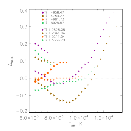
For the A-type stars the LTE abundances from strong lines of Ti ii are higher than those from the weak lines (see Fig. 6 for HD 145788). Such a behavior can be wrongly interpreted as an underestimation of a microturbulent velocity. For example, to derive consistent LTE abundances from different lines of Ti ii in HD 145788 one needs to adopt a microturbulent velocity of = 1.8 km s-1, while = 1.3 km s-1 was found by Fossati et al. (2009) from lines of Fe ii. We show that a discrepancy between strong and weak lines vanishes in NLTE. This is because the strong lines are more affected by NLTE compared with the weak lines. For example, in HD 145788, the cores of the Ti ii lines with 100 mÅ form at the optical depth log –2.5, and their NLTE abundance corrections reach –0.24 dex. For the Ti ii lines with 70 mÅ the NLTE abundance corrections do not exceed few hundredths in absolute value. We do not recommend to apply the Ti ii lines with 70 mÅ for abundance determination under the LTE assumption. For A-B type stars NLTE leads to significant decrease of line-to-line scatter compared to LTE (Table 5).
We checked effects of the use of accurate photoionisation cross-sections by Nahar (2015) and K. Butler instead of the hydrogenic approximation. Using quantum-mechanical cross-sections for Ti i leads to increasing the photoionisation rates and the deviations from LTE. For example, the NLTE abundance corrections for Ti i lines increase by 0.01–0.02 dex in the model 9700/4.10/0.4/1.8. In the atmospheres with 10500 K the NLTE abundances derived from the Ti ii lines do not change significantly, when using either accurate or hydrogenic cross-sections. This is due to the fact that mechanism of deviations from LTE for Ti ii is not ruled by the bound-free transitions. For the hottest star of our sample, HD 17081 (B7 IV), where Ti ii is affected by overionisation, we found that using the accurate cross-sections leads to weakened NLTE effects for Ti ii and 0.06 dex smaller NLTE abundance compared with that calculated with the hydrogenic cross-sections. Since we adopt the theoretical approximations to calculate electron collision rates, we perform the test calculations. Test calculations with the model atmosphere 7250/4.20/0.0 show that a hundredfold decrease in electron collision rates results in a 0.05 dex increase in the NLTE abundance from Ti i, and up to 0.06 dex decrease in NLTE abundance from the strongest lines of Ti ii with EW of 150 mÅ.
Thus, analysis of the titanium lines in the hot stars gives an evidence for that our NLTE method gives reliable results.
For the 22 lines of Ti i and 82 lines of Ti ii we calculated the NLTE abundance corrections in a grid of model atmospheres with from 6500 K to 13000 K with a step of 250 K, log = 4, [Fe/H] = 0 and = 2 km s-1. For lines of Ti i the NLTE abundance corrections are positive and vary between 0.0 dex to 0.20 dex (Fig. 7). For Ti ii the NLTE abundance corrections are negative for 10000 K and can be up to dex. In the atmospheres with 10000 K the lines of neutral titanium can not be detected, and the NLTE abundance corrections for lines of Ti ii are positive and reach 0.37 dex. The data are available as on-line material (Table 3).
| 1, K | 2 | … | 26 | 27 |
| EW1, mÅ | EW2 | … | EW26 | EW27 |
| 1 | 2 | … | 26 | 27 |
| 6500 | 6750 | … | 12750 | 13000 |
| … | ||||
| 5210.3838 Å Ti i = 0.048 eV log gf = –0.820 | ||||
| 54 | 40 | … | –1 | –1 |
| 0.17 | 0.17 | … | –1.00 | –1.00 |
| … | ||||
| 4395.0308 Å Ti ii = 1.084 eV log gf = –0.540 | ||||
| 176 | 169 | … | 15 | 12 |
| –0.09 | –0.10 | … | 0.25 | 0.26 |

5 Analysis of Ti i and Ti ii lines in the reference late-type stars
5.1 Ti i and Ti ii lines in the solar spectrum
We used 27 Ti i and 12 Ti ii lines in the solar flux spectrum (Kurucz et al., 1984) to determine the LTE and NLTE abundances. Under the LTE assumption we derived log A 0.06 dex and log A 0.04 dex from the lines of Ti i and Ti ii, respectively. We calculated the NLTE abundances for = 0, 0.1, 0.5 and 1.0. Consistent within 0.03 dex abundances from Ti i and Ti ii were found in NLTE, independent of adopted value (Table 4). This means that the solar analysis does not help to constrain . Solar titanium abundance averaged over Ti i and Ti ii lines, log A = 0.06 (NLTE, = 1), agrees with the meteoritic value, log A = 0.03 dex (Lodders et al., 2009).
The treated NLTE method was applied before publication to check the Ti i/Ti ii ionisation equilibrium of 11 stars with 5050 6600 K, 3.76 log 4.47 and [Fe/H] (Ryabchikova et al., 2016). For HD 49933 (6600/4.0/), the star with the largest deviations from LTE in the sample, the NLTE calculations provide consistent within the error bars the Ti i and Ti ii based abundances independent of using either = 0.5 or 1. For the studied stars the NLTE abundance difference Ti i–Ti ii nowhere exceeds dex.
5.2 Ti i and Ti ii lines in the metal-poor stars
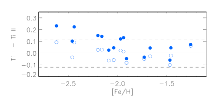
Metal-poor stars suit better for a calibration of parameter than the solar-metallicity stars. This is due to the deviations from LTE grow with decreasing [Fe/H] because of increasing the ultraviolet (UV) flux and decreasing electronic number density. Our sample of cool MP dwarfs includes 15 stars with [Fe/H] . For all the stars we determined the titanium abundance under the LTE assumption and in NLTE with = 1.0, and also with = 0.5 and 0.1 for few stars. The abundance differences Ti i–Ti ii are listed in Table 4 for various line formation scenarios and shown in Fig. 9 for LTE and NLTE with = 1.0. For the seven stars the NLTE calculations result in consistent within the error bars abundances from Ti i and Ti ii. For example, in HD 94028 Ti i–Ti ii = dex in LTE, and reduces to dex in NLTE ( = 1). For the other eight stars, on the contrary, an agreement between Ti i and Ti ii is better in LTE compared to that in NLTE. Moreover, for these stars Ti i–Ti ii 0 is obtained already in LTE, and the difference increases in NLTE. For example, in BD we derived the largest discrepancy of 0.23 dex when using NLTE with = 1, while in LTE Ti i–Ti ii = 0.09 dex. All these stars, except HD 103095, are either turn-off (TO) stars with 6200 6400 K, 3.9 log 4.1, [Fe/H], or VMP subgiants (SG) with 5780 K. Due to lower leads to larger NLTE effects, we do not perform calculations with 1 for these stars, except HD 84937. For the eight dwarfs with negative LTE abundance difference Ti i–Ti ii we performed NLTE calculations with = 0.5. The minimal difference Ti i–Ti iifor maximal number of stars is achieved, when using = 1.
HD 122563 (MP giant). In LTE we derived an abundance difference of Ti i–Ti ii dex, and in NLTE it decreases in absolute value and amounts to Ti i–Ti ii dex, dex, and dex, when using = 1.0, 0.5, and 0.1, respectively. To achieve an agreement between Ti i and Ti ii, the lower is required, compared with that for the dwarfs. It is worth noting that similar conclusion was drawn by Mashonkina et al. (2011) from a relative to the Sun line-by-line differential analysis of iron lines in HD 122563. Mashonkina et al. (2011) derived an abundance difference of Fe i–Fe ii dex in LTE and Fe i–Fe ii dex, dex, and 0.03 dex in NLTE, when using = 1.0, 0.1, and 0.0, respectively. While to achieve the Fe i/Fe ii balance for MP TO-star HD 84937 = 1 is required. In HD 122563, for both Fe i and Fe ii and Ti i and Ti ii NLTE leads to smaller abundance difference between the two ionisation stages compared to LTE.
5.3 Comparison with other studies
We have the four stars in common with Bergemann (2011), namely, the Sun, HD 84937, HD140283, and HD 122563. For the common lines of Ti i and Ti ii used in the solar analyses we recalculated abundances derived by Bergemann (2011) using gf-values adopted in this study. For the majority lines the LTE abundance difference between Bergemann (2011) and our data does not exceed 0.03 dex and nowhere exceeds 0.05 dex. We also compared the NLTE abundance corrections for Ti i. Bergemann (2011) adopted = 3 in the NLTE calculations, while we use = 1. However, for the majority lines she computed larger NLTE abundance corrections, by up to 0.03 dex (for Ti i 4981Å). Bergemann (2011) derived with = 3 the average abundance difference Ti iNLTE–Ti iLTE = 0.05 dex, while we obtain the same value, when using = 0.5. The smaller NLTE effects in this study compared with Bergemann (2011) are due to using a comprehensive model atom that includes predicted high-excitation levels of Ti i.
The difference between our and Bergemann (2011) NLTE results grows, when moving to the MP stars. We compare the abundance differences Ti iNLTE–Ti iLTE and Ti i-Ti ii. For HD 84937, Bergemann (2011) derived Ti iNLTE–Ti iLTE = 0.14 dex using = 3 and MAFAGS-OS model atmosphere (Grupp et al., 2009). Using the same stellar parameters for this star, = 3, and MARCS model atmosphere (Gustafsson et al., 2008) we derived Ti iNLTE–Ti iLTE = 0.09 dex. We checked, whether this abundance discrepancy can be attributed to different codes for model atmosphere calculation. We calculated Ti i and Ti ii abundances with MARCS and MAFAGS-OS models, and found that the abundance difference does not exceed 0.02 dex for any line. For HD 84937 Bergemann (2011) derived in LTE Ti i–Ti ii = 0.11 dex, while we found Ti i–Ti ii dex. For HD 140283 she presents abundances calculated only with the MAFAGS-ODF model structure, Ti i–Ti ii = 0.02 dex in LTE and 0.16 dex in NLTE ( = 3). The corresponding values in our calculations are dex (LTE) and 0.09 dex (NLTE, = 1). Similar situation in our studies was found for HD 122563. We derived discrepancies of Ti i–Ti ii dex and dex in LTE and NLTE ( = 1), respectively. The corresponding LTE and NLTE ( = 3) values from Bergemann (2011) are dex and dex. This abundance comparison indicates that our model atom leads to smaller deviations from LTE compared with those computed by Bergemann (2011).
The star HD 84937 is used like a reference star in many studies, since its atmospheric parameters are well-determined by different independent methods. Sneden et al. (2016) investigated the titanium lines under the LTE assumption adopting = 6300 K, log g = 4.0, [Fe/H], = 1.5 km s-1 and the interpolated model from Kurucz (2011) model grid. In LTE they found consistent abundances from Ti i and Ti ii. Using adopted in their study atmospheric parameters and our linelist we derived in LTE Ti iTi ii = 0.02 dex. A very similar abundance difference of Ti i–Ti ii = 0.03 dex was found, with our parameters 6350/4.09//1.7. This is due to higher and higher log lead to decrease in abundance from Ti i and Ti ii, respectively, keeping the ionisation balance safe. HD 84937 is one of the stars, where NLTE leads to positive Ti i–Ti iiabundance difference, as discussed above.
5.4 What is a source of discrepancy between Ti i and Ti ii in VMP TO-stars?
The treatment of collisions with H i. The main NLTE mechanism for Ti i is the UV overionisation and there is no process, which can result in strengthened lines of Ti i and negative NLTE abundance corrections. Inelastic collisions with H i atoms serve as an additional source of thermalisation that reduces, but does not cancel the overionisation. It is worth noting that in the atmospheres of our VMP ([Fe/H] ) TO-stars the lines of Ti i are weak (EW 20 mÅ) and form inwards log = . The NLTE abundance corrections for Ti ii lines are positive in the model 6350/4.09/, 0.01 dex when = 1, and can be up to 0.08 dex, when neglecting collisions with H i atoms. To what extent inelastic collisions with H i atoms can help to solve the problem of Ti i–Ti ii in the MP TO stars remains unclear until accurate collisional data will be computed for both Ti i + H i and Ti ii + H i.
Uncertainties in . The lines of Ti i are more sensitive to variation compared with Fe i lines, because of lower ionisation threshold for Ti i compared to Fe i. For example, we found an abundance shift of 0.09 dex for Ti i lines, and only 0.05 dex for Fe i, when adopting 70 K lower for HD 103095 (5130/4.66/). For this star, a downward revision of by 70 K results in consistent abundances from Ti i and Ti ii, and does not destroy Fe i/Fe ii ionisation equilibrium. However, a different situation was found for the VMP TO stars. For example, we obtained similar abundance shifts of 0.08 dex and 0.06 dex for Ti i and Fe i, respectively, when adopting 100 K lower for HD 84937 (6350/4.09/). For this star, the decrease results in the ionisation equilibrium for titanium, but not for iron.
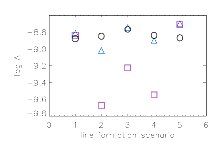
3D effects. The solution of the NLTE problem with such a comprehensive model atom as treated in this study is only possible, at present, with classical plane-parallel (1D) model atmospheres. Neglecting atmospheric inhomogeneities (3D effects) can lead to errors in our results. From hydrodynamical modelling of stellar atmospheres Collet et al. (2007) and Dobrovolskas et al. (2013) predict negative abundance corrections = log A3D–log A1D for lines of neutral species in red giant stars. In the models of TO (5900/4.0) stars with [Fe/H], increases in absolute value with decreasing the excitation energy of the lower level, and reaches dex and dex for the = 4000 Å lines with = 0 and 2 eV, respectively (Dobrovolskas, 2013). All the lines of Ti i used for our MP TO stars have 1.75 eV. The 3D abundance corrections can be either positive or negative, and do not exceed 0.07 dex in absolute value for the lines of Ti ii. Negative 3D corrections for Ti i could help to achieve an agreement between Ti i and Ti ii. We selected two lines of Ti i, at 4617 Å ( = 1.75 eV) and 4681 Å ( = 0.05 eV), and Ti ii 5336 Å ( = 1.58 eV), which give consistent within 0.02 dex LTE abundances and calculated the abundance differences Ti i–Ti iifor different line formation scenarios, taking 3D abundance corrections from Dobrovolskas (2013). Abundances from individual lines are shown in Fig. 8. In LTE we derived Ti i–Ti ii = 0.05 dex and dex in 1D and 3D, respectively. In NLTE+3D we derived dex ( = 1) and dex ( = 0), while Ti i–Ti ii= 0.17 dex in NLTE( = 1)+1D, which is our standard scenario. The predicted 3D effects are too strong for low-excitation lines of Ti i and produce a large discrepancy between Ti i lines with different , which reaches 0.66 dex in LTE+3D. We suppose that for MP stars simple co-adding the NLTE(1D) and 3D(LTE) corrections is too rough procedure, because both NLTE and 3D effects are equally significant.
Chromospheres. One more source can be connected with a star’s chromosphere that heats the line formation layers. An inspiring insight into this problem was presented by Dupree et al. (2016). Further efforts should be invested to evaluate a possible influence of the star’s chromosphere on the formation of titanium lines.
| NLTE, | ||||
|---|---|---|---|---|
| —————————– | ||||
| Star | LTE | 1 | 0.5 | 0.1 |
| Sun | –0.05 | –0.03 | –0.02 | 0.00 |
| HD 64090 | –0.04 | –0.01 | 0.00 | 0.06 |
| HD 84937 | 0.03 | 0.15 | 0.19 | 0.24 |
| HD 94028 | –0.11 | –0.05 | –0.03 | 0.05 |
| HD 122563 | –0.36 | –0.18 | –0.13 | –0.06 |
| BD+07∘ 4841 | –0.06 | 0.02 | 0.06 | |
| BD+09∘ 0352 | –0.06 | 0.04 | 0.08 | |
| HD 140283 | –0.05 | 0.09 | 0.14 | |
| BD+29∘ 2091 | –0.14 | –0.09 | –0.07 | |
| G 090-003 | –0.07 | 0.05 | 0.09 | |
| HD 24289 | 0.00 | 0.14 | ||
| HD 74000 | 0.01 | 0.12 | ||
| HD 103095 | 0.06 | 0.07 | ||
| HD 108177 | –0.07 | 0.02 | ||
| BD–13∘ 3442 | 0.09 | 0.23 | ||
| BD–04∘ 3208 | 0.02 | 0.15 | ||
| BD+24∘ 1676 | 0.07 | 0.20 | ||

| Star | NTiI | log A(Ti i)LTE | log A(Ti i)NLTE | NTiII | log A(Ti ii)LTE | log A(Ti ii)NLTE |
|---|---|---|---|---|---|---|
| HD 37594 | 8 | –7.230.13 | –7.110.11 | 27 | –7.010.15 | –7.040.11 |
| HD 32115 | 6 | –7.450.05 | –7.310.05 | 9 | –7.230.07 | –7.260.05 |
| HD 72660 | 5 | –6.630.05 | –6.570.08 | 36 | –6.540.12 | –6.590.08 |
| HD 73666 | 2 | –6.940.02 | –6.890.09 | 6 | –6.720.20 | –6.840.09 |
| HD 145788 | 32 | –6.760.15 | –6.810.07 | |||
| Sirius | 6 | –6.840.06 | –6.890.04 | |||
| 21 Peg | 46 | –7.240.05 | –7.240.04 | |||
| Cet | 11 | –7.410.09 | –7.140.08 | |||
| Sun | 27 | –7.110.05 | –7.090.05 | 12 | –7.060.04 | –7.060.04 |
| BD–13∘ 3442 | 3 | -9.250.04 | -9.090.04 | 15 | -9.340.06 | -9.320.06 |
| BD–04∘ 3208 | 9 | -8.900.05 | -8.770.05 | 17 | -8.920.06 | -8.920.05 |
| BD+7∘ 4841 | 26 | –8.240.05 | –8.170.05 | 34 | –8.170.06 | –8.190.05 |
| BD+9∘ 0352 | 9 | –8.870.05 | –8.780.05 | 22 | –8.810.05 | –8.820.04 |
| BD+24∘ 1676 | 7 | -9.120.06 | -8.980.06 | 16 | -9.190.06 | -9.180.06 |
| BD+29∘ 2091 | 20 | –8.760.06 | –8.720.06 | 24 | –8.620.08 | –8.630.07 |
| HD 24289 | 16 | –8.790.10 | –8.670.10 | 27 | –8.790.08 | –8.810.09 |
| HD 64090 | 35 | –8.730.07 | –8.710.07 | 30 | –8.690.06 | –8.700.05 |
| HD 74000 | 15 | -8.780.07 | -8.680.07 | 26 | -8.790.08 | -8.800.08 |
| HD 84937 | 12 | –8.840.04 | –8.710.04 | 15 | –8.870.08 | –8.860.08 |
| HD 94028 | 26 | –8.340.06 | –8.300.07 | 26 | –8.230.04 | –8.240.05 |
| HD 103095 | 37 | –8.060.09 | –8.050.09 | 29 | –8.120.07 | –8.120.07 |
| HD 108177 | 14 | –8.500.06 | –8.430.07 | 12 | –8.430.07 | –8.450.06 |
| HD 122563 | 22 | –9.820.07 | –9.640.08 | 36 | –9.460.06 | –9.460.07 |
| HD 140283 | 19 | –9.360.07 | –9.210.07 | 25 | –9.310.05 | –9.300.05 |
| G 090–03 | 18 | –8.850.07 | –8.750.07 | 30 | –8.780.07 | –8.790.06 |
| For the cool stars the NLTE abundances were derived using = 1. | ||||||
6 Conclusions
We construct a comprehensive model atom for Ti i– ii using the energy levels from laboratory measurements and theoretical predictions and quantum mechanical photoionisation cross-sections. NLTE line formation for Ti i and Ti ii lines was considered in 1D-LTE model atmospheres of the 25 reference stars with reliable stellar parameters, which cover a broad range of effective temperatures 4600 12800 K, surface gravities 1.60 log 4.70, and metallicities [Fe/H] +0.4.
The NLTE calculations for Ti i– ii in A-type stars were performed for the first time. The NLTE titanium abundances were determined for the eight stars. For the four stars with both Ti i and Ti ii lines observed, NLTE analysis provides consistent within 0.07 dex abundances from Ti i and Ti ii lines, while the corresponding LTE abundance difference can be up to 0.22 dex in absolute value. For each species, NLTE leads to smaller line-to-line scatter compared with LTE. For stars with 7000 K lines of Ti i and Ti ii can be used for atmospheric parameter determination, when taking into account deviations from LTE. For the 22 lines of Ti i and 82 lines of Ti ii we calculated the NLTE abundance corrections in a grid of model atmospheres with from 6500 K to 13000 K, log = 4, [Fe/H] = 0, and =2 km s-1.
We made progress in determination of NLTE abundance of titanium for cool stars compared with data from the literature. Taking into account a bulk of the predicted high-excitation levels of Ti i in the model atom established close collisional coupling of the Ti i levels near the continuum to the ground state of Ti ii resulting in smaller NLTE effects in cool model atmospheres compered with the Bergemann (2011) data. Because no accurate calculations of inelastic collisions of titanium with neutral hydrogen atoms are available, we use the Drawinian formalism with the scaling factor, which was estimated as = 1 from abundance comparison between Ti i and Ti ii in the sample of cool main sequence stars over wide metallicity range, [Fe/H] 0.0. For the VMP TO-stars NLTE fails to achieve agreement between Ti i and Ti ii. Moreover, for these stars we derived positive abundance difference Ti i–Ti iiin LTE, and it increases in NLTE. To clarify this matter, accurate collisional data for Ti i and Ti ii would be extremely helpful.
7 Appendix
This is a full version of Table 1. The list of Ti i and Ti ii lines with the adopted atomic data.
(Å), (eV), log gf, transition, log , log , log
Ti I
4008.927 0.021 -1.000 3a3F – y3F 8.000 -6.080 -7.750
4060.262 1.052 -0.690 a3P – x3P 8.050 -6.050 -7.646
4060.262 1.052 -0.690 a3P – x3P 8.050 -6.050 -7.646
4287.403 0.836 -0.370 a5F – x5D 8.230 -6.010 -7.570
4449.143 1.886 0.470 a3G – v3G 8.120 -5.560 -7.579
4453.699 1.872 0.100 a3G – v3G 8.110 -4.970 -7.582
4512.733 0.836 -0.400 a5F – y5F 8.130 -5.120 -7.593
4533.240 0.848 0.540 a5F – y5F 8.130 -5.120 -7.593
4534.776 0.836 0.350 a5F – y5F 8.130 -5.280 -7.596
4548.763 0.826 -0.280 a5F – y5F 8.130 -5.410 -7.598
4555.484 0.848 -0.400 a5F – y5F 8.130 -5.280 -7.596
4617.268 1.748 0.440 a5P – w5D 8.080 -5.860 -7.626
4623.097 1.739 0.160 a5P – w5D 8.070 -5.850 -7.627
4639.361 1.739 -0.050 a5P – w5D 8.070 -5.840 -7.740
4639.661 1.748 -0.140 a5P – w5D 8.070 -5.850 -7.740
4639.940 1.733 -0.160 a5P – w5D 8.070 -5.840 -7.630
4656.468 0.000 -1.2902 2a3F – z3G 6.380 -6.110 -7.706
4681.909 0.050 -1.0302 4a3F – z3G 6.460 -6.110 -7.702
4758.118 2.248 0.510 a3H – x3H 8.080 -6.040 -7.621
4759.269 2.255 0.590 a3H – x3H 8.080 -6.040 -7.620
4820.410 1.502 -0.380 a1G – y1F 8.210 -5.940 -7.625
4840.874 0.899 -0.430 a1D – y1D 7.530 -6.120 -7.697
4913.615 1.872 0.220 a3G – y3H 7.850 -5.890 -7.619
4981.731 0.848 0.570 a5F – y5G 7.950 -6.050 -7.626
4991.067 0.836 0.450 a5F – y5G 7.940 -6.050 -7.629
4997.093 0.000 -2.070 2a3F – z3D 6.900 -6.110 -7.722
4999.502 0.826 0.320 a5F – y5G 7.940 -6.050 -7.632
5009.645 0.021 -2.200 3a3F – z3D 6.870 -6.110 -7.720
5016.161 0.848 -0.480 a5F – y5G 7.940 -6.050 -7.629
5020.025 0.836 -0.330 a5F – y5G 7.940 -6.050 -7.630
5024.844 0.818 -0.530 a5F – y5G 7.940 -6.050 -7.635
5025.570 2.041 0.2501 z5G – e5F 7.960 -5.310 -7.550
5036.464 1.443 0.140 b3F – w3G 8.160 -5.700 -7.539
5039.955 0.021 -1.080 3a3F – z3D 6.900 -6.110 -7.720
5064.652 0.048 -0.940 4a3F – z3D 6.870 -6.110 -7.719
5147.477 0.000 -1.940 2a3F – z3F 6.820 -6.110 -7.727
5173.740 0.000 -1.060 2a3F – z3F 6.820 -6.110 -7.729
5192.969 0.021 -0.950 3a3F – z3F 6.820 -6.110 -7.727
5210.384 0.048 -0.820 4a3F – z3F 6.810 -6.110 -7.724
5512.524 1.460 -0.400 b3F – w3D 8.190 -6.100 -7.700
5514.343 1.429 -0.660 b3F – w3D 8.140 -5.990 -7.710
5514.532 1.443 -0.500 b3F – w3D 8.150 -6.070 -7.710
5866.449 1.066 -0.790 a3P – y3D 8.000 -6.070 -7.724
6258.099 1.443 -0.390 b3F – y3G 8.250 -5.990 -7.582
6261.096 1.429 -0.530 b3F – y3G 8.260 -5.980 -7.585
8426.506 0.826 -1.2002 a5F – z5D 6.370 -6.090 -7.711
Ti II
2827.114 3.687 -0.0204 z4G – e4G 8.850 -5.850 -7.720
2828.077 3.749 0.8703 z4G – e4H 8.860 -5.820 -7.720
2834.011 3.716 0.0004 z4G – e4G 8.850 -5.850 -7.720
2841.935 0.607 -0.590 a2F – y2F 8.420 -6.390 -7.830
2851.101 1.221 -0.730 a2P – x2D 8.320 -6.470 -7.820
2853.931 0.607 -1.550 a2F – y2F 8.350 -6.390 -7.840
2868.741 0.574 -1.380 a2F – y2D 8.260 -6.390 -7.850
4012.385 0.574 -1.780 a2F – z4G 8.220 -6.390 -7.860
4028.343 1.891 -0.920 b2G – y2F 8.420 -6.410 -7.830
4053.820 1.892 -1.070 b2G – y2F 8.350 -6.410 -7.840
4161.530 1.084 -2.090 a2D – z4D 8.410 -6.430 -7.840
4163.640 2.589 -0.130 b2F – x2D 8.320 -6.470 -7.820
4174.070 2.598 -1.2604 b2F – x2D 8.320 -6.470 -7.820
4188.987 5.423 -0.6004 y2G – e2G 8.900 -5.690 -7.690
4190.233 1.084 -3.1221 a2D – z4D 8.410 -6.430 -7.840
4287.870 1.080 -1.7904 a2D – z2D 8.170 -6.430 -7.850
4290.215 1.164 -0.870 a4P – z4D 8.410 -6.500 -7.840
4300.049 1.180 -0.460 a4P – z4D 8.410 -6.490 -7.840
4301.920 1.160 -1.210 a4P – z4D 8.410 -6.490 -7.840
4316.794 2.047 -1.620 b2P – z2P 8.420 -6.460 -7.840
4337.915 1.080 -0.9604 a2D – z2D 8.160 -6.430 -7.850
4374.820 2.060 -1.570 b2P – y2D 8.260 -6.460 -7.850
4386.844 2.598 -0.9604 b2F – y2G 8.450 -6.540 -7.830
4391.020 1.231 -2.300 b4P – z4D 8.410 -6.410 -7.840
4394.059 1.221 -1.770 a2P – z4D 8.410 -6.490 -7.840
4395.031 1.084 -0.540 a2D – z2F 8.160 -6.430 -7.850
4395.839 1.242 -1.930 b4P – z4D 8.410 -6.410 -7.840
4399.772 1.236 -1.200 a2P – z4D 8.410 -6.500 -7.840
4409.235 1.242 -2.780 b4P – z4D 8.410 -6.410 -7.840
4409.520 1.231 -2.530 b4P – z4D 8.410 -6.410 -7.840
4411.070 3.093 -0.650 c2D – x2F 8.290 -6.330 -7.840
4411.925 1.224 -2.620 b4P – z4D 8.420 -6.410 -7.840
4417.713 1.165 -1.1904 a4P – z2D 8.170 -6.580 -7.850
4418.331 1.236 -1.990 a2P – z4D 8.410 -6.490 -7.840
4421.938 2.060 -1.640 b2P – z2P 8.350 -6.460 -7.840
4423.239 1.231 -3.0661 b4P – z4D 8.420 -6.410 -7.840
4432.109 1.236 -3.080 a2P – z4D 8.420 -6.490 -7.840
4441.730 1.180 -2.3304 a4P – z2D 8.170 -6.580 -7.850
4443.801 1.080 -0.710 a2D – z2F 8.150 -6.430 -7.850
4444.554 1.115 -2.200 a2G – z2F 8.160 -6.590 -7.850
4450.482 1.084 -1.520 a2D – z2F 8.150 -6.430 -7.850
4464.449 1.161 -1.8104 a4P – z2D 8.160 -6.600 -7.850
4468.500 1.130 -0.630 a2G – z2F 8.860 -5.710 -7.690
4468.510 1.130 -0.630 a2G – z2F 8.860 -5.710 -7.690
4469.151 1.084 -2.550 a2D – z4F 8.380 -6.430 -7.840
4470.853 1.165 -2.0204 a4P – z2D 8.160 -6.600 -7.850
4488.324 3.122 -0.500 c2D – x2F 8.280 -6.330 -7.840
4501.270 1.115 -0.770 a2G – z2F 8.150 -6.590 -7.850
4518.330 1.080 -2.560 a2D – z4F 8.380 -6.430 -7.840
4529.474 1.571 -1.750 a2H – z2G 8.310 -6.490 -7.820
4533.960 1.237 -0.5304 a2P – z2D 8.170 -6.540 -7.850
4544.020 1.243 -2.5804 a2G – z4F 8.170 -6.410 -7.850
4549.620 1.583 -0.220 a2H – z2G 8.310 -6.490 -7.820
4563.757 1.221 -0.7951 a2P – z2D 8.160 -6.550 -7.850
4568.314 1.224 -3.0305 b4P – z2D 8.160 -6.410 -7.850
4571.971 1.571 -0.310 a2H – z2G 8.310 -6.490 -7.820
4583.410 1.164 -2.840 a4P – z2F 8.150 -6.590 -7.850
4589.958 1.237 -1.6205 a2P – z2D 8.160 -6.540 -7.850
4636.320 1.165 -3.0241 a4P – z4F 8.380 -6.500 -7.840
4657.201 1.242 -2.290 b4P – z2F 8.160 -6.410 -7.850
4708.663 1.236 -2.350 a2P – z2F 8.150 -6.540 -7.850
4719.515 1.242 -3.320 b4P – z2F 8.150 -6.410 -7.850
4763.880 1.221 -2.400 a2P – z4F 8.380 -6.510 -7.840
4764.525 1.236 -2.690 a2P – z4F 8.380 -6.500 -7.840
4779.985 2.048 -1.2605 b2P – z2S 8.230 -6.460 -7.860
4798.530 1.080 -2.660 a2D – z4G 8.220 -6.430 -7.860
4805.085 2.061 -0.9605 b2P – z2S 8.230 -6.460 -7.860
4865.612 1.115 -2.700 a2G – z4G 8.220 -6.490 -7.860
4911.190 3.122 -0.640 c2D – y2P 8.260 -6.330 -7.830
4996.367 1.582 -3.2906 b2D2 – z4D 8.410 -6.490 -7.840
5005.157 1.565 -2.730 b2D2 – z4D 8.410 -6.490 -7.840
5010.210 3.093 -1.350 c2D – x2D 8.320 -6.330 -7.820
5013.330 3.095 -2.0281 c2D – x2D 8.320 -6.330 -7.820
5013.686 1.581 -2.140 b2D2 – z4D 8.410 -6.500 -7.840
5072.290 3.122 -1.020 c2D – x2D 8.320 -6.330 -7.820
5129.160 1.891 -1.340 b2G – z2G 8.310 -6.410 -7.820
5154.070 1.566 -1.7504 b2D2 – z2D 8.170 -6.580 -7.850
5185.913 1.892 -1.410 b2G – z2G 8.310 -6.410 -7.820
5188.680 1.582 -1.0504 b2D2 – z2D 8.170 -6.580 -7.850
5211.536 2.589 -1.410 b2F – y2F 8.420 -6.480 -7.830
5226.550 1.570 -1.2604 b2D2 – z2D 8.160 -6.590 -7.850
5262.140 1.582 -2.2504 b2D2 – z2D 8.160 -6.590 -7.850
5268.610 2.597 -1.610 b2F – y2F 8.350 -6.480 -7.840
5336.786 1.581 -1.600 b2D2 – z2F 8.160 -6.590 -7.850
5381.022 1.565 -1.970 b2D2 – z2F 8.150 -6.590 -7.850
5418.768 1.581 -2.130 b2D2 – z2F 8.150 -6.590 -7.850
5490.690 1.566 -2.6631 b2D2 – z4F 8.380 -6.510 -7.840
6491.566 2.061 -1.9421 b2P – z2D 8.170 -6.460 -7.850
6606.950 2.060 -2.7903 b2P – z2D 8.160 -6.460 -7.850
6680.133 3.093 -1.890 c2D – y2F 8.350 -6.330 -7.840
6998.905 3.122 -1.280 c2D – y2D 8.260 -6.330 -7.850
sources of gf-values
1 - Kurucz,
2 - BLNP, Blackwell-Whitehead, R. J. and Lundberg, H. and Nave, G. and Pickering, J. C. and Jones, H. R. A. and Lyubchik, Y. and Pavlenko, Y. V. and Viti, S., Monthly Notices Roy. Astron. Soc., 373, 1603-1609 (2006);
3 - MFW, Martin, G.A. and Fuhr, J.R. and Wiese, W.L., J. Phys. Chem. Ref. Data Suppl., 17, 3 (1988);
4 - PTP, Pickering, J. C. and Thorne, A. P. and Perez, R., Astrophys. J. Suppl. Ser., 132, 403-409 (2001);
5 - RHL, Ryabchikova, T. A. and Hill, G. M. and Landstreet, J. D. and Piskunov, N. and Sigut, T. A. A., Monthly Notices Roy. Astron. Soc., 267, 697 (1994);
6 - BHN, Bizzarri, A. and Huber, M. C. E. and Noels, A. and Grevesse, N. and Bergeson, S. D. and Tsekeris, P. and Lawler, J. E., Astronomy and Astrophysics, 273, 707 (1993);
gf-values taken from Wisconsin (Lawler et al., 2013; Wood
et al., 2013) if not prescribed.
This is a full version of Table 3. NLTE abundance corrections and equivalent widths for the lines of Ti i and Ti ii depending on in the models with log = 4, [Fe/H] = 0, and = 2 km s-1. A portion is shown here for guidance regarding its form and content. If EW = and = , this means that EW 5 mÅ in a given model atmosphere.
Calculations are performed for the 27 following effective temperatures (K):
6500 6750 7000 7250 7500 7750 8000 8250 8500 8750 9000 9250 9500 9750 10000 10250 10500 10750 11000 11250 11500 11750 12000 12250 12500 12750 13000
The file is constructed as following:
wavelength, A; Ti species; excitation energy, eV; gf-value
equivalent width1; …; equivalent width27
NLTE abundance correction1; …; NLTE abundance correction27
4287.4028 A Ti1 Eexc = 0.836 log gf = -0.370
38 29 21 15 11 7 5 -1 -1 -1 -1 -1 -1 -1 -1 -1 -1 -1 -1 -1 -1 -1 -1 -1 -1 -1 -1
0.11 0.10 0.09 0.08 0.08 0.08 0.08 -1.00 -1.00 -1.00 -1.00 -1.00 -1.00 -1.00 -1.00 -1.00 -1.00 -1.00 -1.00 -1.00 -1.00 -1.00 -1.00 -1.00 -1.00 -1.00 -1.00
4453.6992 A Ti1 Eexc = 1.872 log gf = 0.100
18 13 10 7 5 -1 -1 -1 -1 -1 -1 -1 -1 -1 -1 -1 -1 -1 -1 -1 -1 -1 -1 -1 -1 -1 -1
0.14 0.13 0.12 0.12 0.12 -1.00 -1.00 -1.00 -1.00 -1.00 -1.00 -1.00 -1.00 -1.00 -1.00 -1.00 -1.00 -1.00 -1.00 -1.00 -1.00 -1.00 -1.00 -1.00 -1.00 -1.00 -1.00
4512.7329 A Ti1 Eexc = 0.836 log gf = -0.400
38 28 21 15 10 7 5 -1 -1 -1 -1 -1 -1 -1 -1 -1 -1 -1 -1 -1 -1 -1 -1 -1 -1 -1 -1
0.10 0.09 0.08 0.08 0.08 0.08 0.09 -1.00 -1.00 -1.00 -1.00 -1.00 -1.00 -1.00 -1.00 -1.00 -1.00 -1.00 -1.00 -1.00 -1.00 -1.00 -1.00 -1.00 -1.00 -1.00 -1.00
4533.2402 A Ti1 Eexc = 0.848 log gf = 0.540
94 82 72 60 49 37 27 18 12 7 -1 -1 -1 -1 -1 -1 -1 -1 -1 -1 -1 -1 -1 -1 -1 -1 -1
0.04 0.05 0.05 0.06 0.07 0.08 0.09 0.10 0.11 0.11 -1.00 -1.00 -1.00 -1.00 -1.00 -1.00 -1.00 -1.00 -1.00 -1.00 -1.00 -1.00 -1.00 -1.00 -1.00 -1.00 -1.00
4534.7759 A Ti1 Eexc = 0.836 log gf = 0.350
86 74 63 52 41 30 21 14 9 5 -1 -1 -1 -1 -1 -1 -1 -1 -1 -1 -1 -1 -1 -1 -1 -1 -1
0.06 0.06 0.06 0.07 0.07 0.08 0.09 0.10 0.11 0.11 -1.00 -1.00 -1.00 -1.00 -1.00 -1.00 -1.00 -1.00 -1.00 -1.00 -1.00 -1.00 -1.00 -1.00 -1.00 -1.00 -1.00
4548.7632 A Ti1 Eexc = 0.826 log gf = -0.280
46 35 26 19 13 9 6 -1 -1 -1 -1 -1 -1 -1 -1 -1 -1 -1 -1 -1 -1 -1 -1 -1 -1 -1 -1
0.10 0.09 0.08 0.08 0.08 0.08 0.09 -1.00 -1.00 -1.00 -1.00 -1.00 -1.00 -1.00 -1.00 -1.00 -1.00 -1.00 -1.00 -1.00 -1.00 -1.00 -1.00 -1.00 -1.00 -1.00 -1.00
4617.2681 A Ti1 Eexc = 1.748 log gf = 0.440
40 31 24 18 13 9 7 -1 -1 -1 -1 -1 -1 -1 -1 -1 -1 -1 -1 -1 -1 -1 -1 -1 -1 -1 -1
0.13 0.13 0.13 0.13 0.12 0.13 0.12 -1.00 -1.00 -1.00 -1.00 -1.00 -1.00 -1.00 -1.00 -1.00 -1.00 -1.00 -1.00 -1.00 -1.00 -1.00 -1.00 -1.00 -1.00 -1.00 -1.00
4656.4678 A Ti1 Eexc = 0.000 log gf = -1.290
25 17 12 8 5 -1 -1 -1 -1 -1 -1 -1 -1 -1 -1 -1 -1 -1 -1 -1 -1 -1 -1 -1 -1 -1 -1
0.20 0.19 0.17 0.16 0.15 -1.00 -1.00 -1.00 -1.00 -1.00 -1.00 -1.00 -1.00 -1.00 -1.00 -1.00 -1.00 -1.00 -1.00 -1.00 -1.00 -1.00 -1.00 -1.00 -1.00 -1.00 -1.00
4759.2690 A Ti1 Eexc = 2.255 log gf = 0.590
26 20 16 12 9 6 5 -1 -1 -1 -1 -1 -1 -1 -1 -1 -1 -1 -1 -1 -1 -1 -1 -1 -1 -1 -1
0.12 0.11 0.10 0.10 0.10 0.09 0.09 -1.00 -1.00 -1.00 -1.00 -1.00 -1.00 -1.00 -1.00 -1.00 -1.00 -1.00 -1.00 -1.00 -1.00 -1.00 -1.00 -1.00 -1.00 -1.00 -1.00
4913.6152 A Ti1 Eexc = 1.872 log gf = 0.220
25 18 14 10 7 5 -1 -1 -1 -1 -1 -1 -1 -1 -1 -1 -1 -1 -1 -1 -1 -1 -1 -1 -1 -1 -1
0.11 0.10 0.10 0.10 0.09 0.09 -1.00 -1.00 -1.00 -1.00 -1.00 -1.00 -1.00 -1.00 -1.00 -1.00 -1.00 -1.00 -1.00 -1.00 -1.00 -1.00 -1.00 -1.00 -1.00 -1.00 -1.00
4981.7310 A Ti1 Eexc = 0.848 log gf = 0.570
106 94 82 70 58 46 34 23 15 9 6 -1 -1 -1 -1 -1 -1 -1 -1 -1 -1 -1 -1 -1 -1 -1 -1
-0.02 -0.01 -0.00 0.02 0.03 0.05 0.07 0.08 0.09 0.09 0.09 -1.00 -1.00 -1.00 -1.00 -1.00 -1.00 -1.00 -1.00 -1.00 -1.00 -1.00 -1.00 -1.00 -1.00 -1.00 -1.00
4999.5020 A Ti1 Eexc = 0.826 log gf = 0.320
89 77 65 53 42 31 22 14 9 6 -1 -1 -1 -1 -1 -1 -1 -1 -1 -1 -1 -1 -1 -1 -1 -1 -1
0.01 0.02 0.03 0.04 0.05 0.06 0.07 0.08 0.09 0.09 -1.00 -1.00 -1.00 -1.00 -1.00 -1.00 -1.00 -1.00 -1.00 -1.00 -1.00 -1.00 -1.00 -1.00 -1.00 -1.00 -1.00
5016.1611 A Ti1 Eexc = 0.848 log gf = -0.480
36 27 19 14 9 6 -1 -1 -1 -1 -1 -1 -1 -1 -1 -1 -1 -1 -1 -1 -1 -1 -1 -1 -1 -1 -1
0.09 0.08 0.07 0.06 0.06 0.07 -1.00 -1.00 -1.00 -1.00 -1.00 -1.00 -1.00 -1.00 -1.00 -1.00 -1.00 -1.00 -1.00 -1.00 -1.00 -1.00 -1.00 -1.00 -1.00 -1.00 -1.00
5025.5698 A Ti1 Eexc = 2.041 log gf = 0.250
20 15 12 9 6 5 -1 -1 -1 -1 -1 -1 -1 -1 -1 -1 -1 -1 -1 -1 -1 -1 -1 -1 -1 -1 -1
0.16 0.14 0.12 0.11 0.09 0.08 -1.00 -1.00 -1.00 -1.00 -1.00 -1.00 -1.00 -1.00 -1.00 -1.00 -1.00 -1.00 -1.00 -1.00 -1.00 -1.00 -1.00 -1.00 -1.00 -1.00 -1.00
5036.4639 A Ti1 Eexc = 1.443 log gf = 0.140
41 31 24 17 13 9 6 -1 -1 -1 -1 -1 -1 -1 -1 -1 -1 -1 -1 -1 -1 -1 -1 -1 -1 -1 -1
0.10 0.09 0.09 0.09 0.08 0.08 0.08 -1.00 -1.00 -1.00 -1.00 -1.00 -1.00 -1.00 -1.00 -1.00 -1.00 -1.00 -1.00 -1.00 -1.00 -1.00 -1.00 -1.00 -1.00 -1.00 -1.00
5173.7402 A Ti1 Eexc = 0.000 log gf = -1.060
41 29 20 13 9 6 -1 -1 -1 -1 -1 -1 -1 -1 -1 -1 -1 -1 -1 -1 -1 -1 -1 -1 -1 -1 -1
0.18 0.17 0.16 0.16 0.15 0.14 -1.00 -1.00 -1.00 -1.00 -1.00 -1.00 -1.00 -1.00 -1.00 -1.00 -1.00 -1.00 -1.00 -1.00 -1.00 -1.00 -1.00 -1.00 -1.00 -1.00 -1.00
5192.9692 A Ti1 Eexc = 0.021 log gf = -0.950
46 33 23 16 11 7 5 -1 -1 -1 -1 -1 -1 -1 -1 -1 -1 -1 -1 -1 -1 -1 -1 -1 -1 -1 -1
0.19 0.19 0.17 0.16 0.15 0.14 0.13 -1.00 -1.00 -1.00 -1.00 -1.00 -1.00 -1.00 -1.00 -1.00 -1.00 -1.00 -1.00 -1.00 -1.00 -1.00 -1.00 -1.00 -1.00 -1.00 -1.00
5210.3838 A Ti1 Eexc = 0.048 log gf = -0.820
54 40 29 20 14 9 6 -1 -1 -1 -1 -1 -1 -1 -1 -1 -1 -1 -1 -1 -1 -1 -1 -1 -1 -1 -1
0.17 0.17 0.17 0.16 0.15 0.14 0.14 -1.00 -1.00 -1.00 -1.00 -1.00 -1.00 -1.00 -1.00 -1.00 -1.00 -1.00 -1.00 -1.00 -1.00 -1.00 -1.00 -1.00 -1.00 -1.00 -1.00
5866.4492 A Ti1 Eexc = 1.066 log gf = -0.790
14 10 7 5 -1 -1 -1 -1 -1 -1 -1 -1 -1 -1 -1 -1 -1 -1 -1 -1 -1 -1 -1 -1 -1 -1 -1
0.15 0.14 0.13 0.13 -1.00 -1.00 -1.00 -1.00 -1.00 -1.00 -1.00 -1.00 -1.00 -1.00 -1.00 -1.00 -1.00 -1.00 -1.00 -1.00 -1.00 -1.00 -1.00 -1.00 -1.00 -1.00 -1.00
6258.0991 A Ti1 Eexc = 1.443 log gf = -0.390
19 14 10 7 5 -1 -1 -1 -1 -1 -1 -1 -1 -1 -1 -1 -1 -1 -1 -1 -1 -1 -1 -1 -1 -1 -1
0.08 0.06 0.05 0.04 0.04 -1.00 -1.00 -1.00 -1.00 -1.00 -1.00 -1.00 -1.00 -1.00 -1.00 -1.00 -1.00 -1.00 -1.00 -1.00 -1.00 -1.00 -1.00 -1.00 -1.00 -1.00 -1.00
6261.0962 A Ti1 Eexc = 1.429 log gf = -0.530
14 10 7 5 -1 -1 -1 -1 -1 -1 -1 -1 -1 -1 -1 -1 -1 -1 -1 -1 -1 -1 -1 -1 -1 -1 -1
0.08 0.06 0.05 0.04 -1.00 -1.00 -1.00 -1.00 -1.00 -1.00 -1.00 -1.00 -1.00 -1.00 -1.00 -1.00 -1.00 -1.00 -1.00 -1.00 -1.00 -1.00 -1.00 -1.00 -1.00 -1.00 -1.00
8426.5059 A Ti1 Eexc = 0.826 log gf = -1.200
16 11 7 5 -1 -1 -1 -1 -1 -1 -1 -1 -1 -1 -1 -1 -1 -1 -1 -1 -1 -1 -1 -1 -1 -1 -1
0.03 0.03 0.02 0.02 -1.00 -1.00 -1.00 -1.00 -1.00 -1.00 -1.00 -1.00 -1.00 -1.00 -1.00 -1.00 -1.00 -1.00 -1.00 -1.00 -1.00 -1.00 -1.00 -1.00 -1.00 -1.00 -1.00
2827.1140 A Ti2 Eexc = 3.687 log gf = -0.020
47 44 41 38 35 31 28 24 20 17 14 12 10 8 7 6 5 -1 -1 -1 -1 -1 -1 -1 -1 -1 -1
0.01 0.01 0.01 0.00 0.00 -0.00 -0.00 -0.00 0.00 0.00 0.01 0.01 0.02 0.03 0.04 0.05 0.07 -1.00 -1.00 -1.00 -1.00 -1.00 -1.00 -1.00 -1.00 -1.00 -1.00
2828.0769 A Ti2 Eexc = 3.749 log gf = 0.870
80 78 75 72 69 66 62 58 54 49 45 40 37 33 30 27 24 22 19 16 14 12 9 8 6 5 -1
0.04 0.03 0.02 0.01 -0.01 -0.02 -0.03 -0.03 -0.03 -0.03 -0.02 -0.01 0.01 0.02 0.04 0.06 0.08 0.09 0.12 0.16 0.20 0.24 0.28 0.32 0.35 0.38 -1.00
2834.0110 A Ti2 Eexc = 3.716 log gf = 0.000
48 45 42 39 36 32 29 25 21 18 15 12 10 8 7 6 5 -1 -1 -1 -1 -1 -1 -1 -1 -1 -1
0.01 0.01 0.01 0.00 0.00 -0.00 -0.00 -0.00 -0.00 0.00 0.01 0.01 0.02 0.03 0.04 0.05 0.07 -1.00 -1.00 -1.00 -1.00 -1.00 -1.00 -1.00 -1.00 -1.00 -1.00
2841.9351 A Ti2 Eexc = 0.607 log gf = -0.590
130 122 115 109 104 98 93 87 82 76 70 65 60 55 51 47 42 37 33 28 23 18 14 11 9 7 5
-0.01 -0.03 -0.04 -0.05 -0.07 -0.09 -0.10 -0.12 -0.13 -0.13 -0.14 -0.14 -0.13 -0.12 -0.10 -0.08 -0.06 -0.04 -0.01 0.02 0.07 0.11 0.16 0.20 0.24 0.28 0.30
2851.1011 A Ti2 Eexc = 1.221 log gf = -0.730
100 96 92 87 82 78 73 67 61 55 49 43 38 33 29 25 21 18 14 12 9 7 5 -1 -1 -1 -1
-0.03 -0.04 -0.05 -0.06 -0.08 -0.09 -0.09 -0.09 -0.09 -0.09 -0.08 -0.07 -0.05 -0.04 -0.03 -0.01 0.00 0.02 0.05 0.08 0.12 0.17 0.21 -1.00 -1.00 -1.00 -1.00
2853.9309 A Ti2 Eexc = 0.607 log gf = -1.550
91 87 82 77 71 66 60 54 47 40 33 28 23 19 15 12 10 8 6 5 -1 -1 -1 -1 -1 -1 -1
-0.02 -0.03 -0.04 -0.04 -0.05 -0.05 -0.05 -0.05 -0.04 -0.04 -0.04 -0.04 -0.03 -0.03 -0.03 -0.02 -0.01 0.00 0.03 0.05 -1.00 -1.00 -1.00 -1.00 -1.00 -1.00 -1.00
2868.7410 A Ti2 Eexc = 0.574 log gf = -1.380
97 93 88 83 78 72 66 60 54 47 41 35 29 25 20 17 14 11 9 7 5 -1 -1 -1 -1 -1 -1
-0.02 -0.03 -0.04 -0.05 -0.06 -0.06 -0.07 -0.07 -0.07 -0.06 -0.06 -0.06 -0.05 -0.05 -0.04 -0.03 -0.02 -0.01 0.01 0.04 0.08 -1.00 -1.00 -1.00 -1.00 -1.00 -1.00
4012.3850 A Ti2 Eexc = 0.574 log gf = -1.780
117 113 108 104 99 95 90 84 77 68 59 51 43 36 29 24 19 15 12 9 7 5 -1 -1 -1 -1 -1
-0.03 -0.03 -0.03 -0.03 -0.03 -0.02 -0.02 -0.02 -0.01 -0.01 -0.01 -0.01 -0.01 -0.01 -0.01 -0.00 0.01 0.02 0.04 0.07 0.10 0.13 -1.00 -1.00 -1.00 -1.00 -1.00
4028.3430 A Ti2 Eexc = 1.891 log gf = -0.920
105 103 100 97 94 90 87 82 76 69 62 54 47 41 35 30 25 21 17 14 11 8 6 5 -1 -1 -1
-0.03 -0.03 -0.03 -0.03 -0.03 -0.03 -0.03 -0.02 -0.02 -0.02 -0.01 -0.01 -0.01 -0.01 -0.00 0.00 0.01 0.02 0.04 0.06 0.09 0.12 0.15 0.17 -1.00 -1.00 -1.00
4053.8201 A Ti2 Eexc = 1.892 log gf = -1.070
98 95 92 89 86 82 78 73 67 60 52 45 38 32 27 23 19 16 12 10 8 6 5 -1 -1 -1 -1
-0.02 -0.03 -0.03 -0.03 -0.03 -0.02 -0.02 -0.01 -0.01 -0.01 -0.01 -0.01 -0.01 -0.01 -0.00 0.00 0.01 0.02 0.04 0.06 0.09 0.12 0.15 -1.00 -1.00 -1.00 -1.00
4161.5298 A Ti2 Eexc = 1.084 log gf = -2.090
84 80 75 70 65 59 52 45 38 31 24 19 15 12 10 7 6 5 -1 -1 -1 -1 -1 -1 -1 -1 -1
-0.02 -0.02 -0.02 -0.02 -0.01 -0.01 -0.01 -0.01 -0.01 -0.01 -0.01 -0.01 -0.00 -0.00 0.00 0.01 0.01 0.03 -1.00 -1.00 -1.00 -1.00 -1.00 -1.00 -1.00 -1.00 -1.00
4163.6401 A Ti2 Eexc = 2.589 log gf = -0.130
116 114 112 110 108 106 103 99 95 89 83 77 70 64 57 51 45 39 33 28 23 19 15 12 10 8 7
-0.04 -0.04 -0.05 -0.05 -0.06 -0.05 -0.05 -0.05 -0.04 -0.04 -0.03 -0.02 -0.01 -0.01 0.00 0.02 0.03 0.05 0.07 0.09 0.13 0.16 0.19 0.22 0.24 0.26 0.28
4174.0698 A Ti2 Eexc = 2.598 log gf = -1.260
54 53 50 47 44 40 37 32 28 23 19 15 13 10 8 7 6 5 -1 -1 -1 -1 -1 -1 -1 -1 -1
0.00 -0.00 -0.00 -0.00 -0.00 -0.00 -0.00 -0.00 -0.00 -0.00 -0.00 0.00 0.00 0.01 0.01 0.02 0.03 0.05 -1.00 -1.00 -1.00 -1.00 -1.00 -1.00 -1.00 -1.00 -1.00
4188.9868 A Ti2 Eexc = 5.423 log gf = -0.600
-1 -1 -1 -1 -1 -1 -1 -1 -1 -1 -1 -1 -1 -1 -1 -1 -1 -1 -1 -1 -1 -1 -1 -1 -1 -1 -1
-1.00 -1.00 -1.00 -1.00 -1.00 -1.00 -1.00 -1.00 -1.00 -1.00 -1.00 -1.00 -1.00 -1.00 -1.00 -1.00 -1.00 -1.00 -1.00 -1.00 -1.00 -1.00 -1.00 -1.00 -1.00 -1.00 -1.00
4190.2329 A Ti2 Eexc = 1.084 log gf = -3.122
24 21 18 15 12 10 8 7 5 -1 -1 -1 -1 -1 -1 -1 -1 -1 -1 -1 -1 -1 -1 -1 -1 -1 -1
-0.00 -0.00 -0.00 -0.00 -0.00 -0.00 -0.00 -0.00 -0.00 -1.00 -1.00 -1.00 -1.00 -1.00 -1.00 -1.00 -1.00 -1.00 -1.00 -1.00 -1.00 -1.00 -1.00 -1.00 -1.00 -1.00 -1.00
4287.8701 A Ti2 Eexc = 1.080 log gf = -1.790
103 99 95 90 85 80 74 67 59 50 41 34 27 22 18 14 11 9 7 5 -1 -1 -1 -1 -1 -1 -1
-0.07 -0.07 -0.06 -0.05 -0.05 -0.04 -0.03 -0.02 -0.02 -0.02 -0.01 -0.01 -0.01 -0.01 -0.00 0.00 0.01 0.03 0.05 0.07 -1.00 -1.00 -1.00 -1.00 -1.00 -1.00 -1.00
4290.2148 A Ti2 Eexc = 1.164 log gf = -0.870
148 143 138 133 129 125 120 115 109 102 95 87 80 73 65 58 50 43 36 30 24 19 14 11 9 7 5
-0.07 -0.08 -0.09 -0.09 -0.09 -0.08 -0.08 -0.07 -0.06 -0.06 -0.05 -0.05 -0.04 -0.03 -0.02 -0.01 0.00 0.01 0.04 0.06 0.10 0.13 0.17 0.20 0.23 0.26 0.27
4300.0488 A Ti2 Eexc = 1.180 log gf = -0.460
176 169 162 156 151 146 141 136 130 123 116 110 103 97 90 83 76 69 61 54 45 37 30 24 19 16 13
-0.06 -0.07 -0.08 -0.09 -0.10 -0.10 -0.10 -0.10 -0.10 -0.09 -0.09 -0.09 -0.08 -0.07 -0.06 -0.05 -0.03 -0.01 0.02 0.05 0.09 0.12 0.16 0.20 0.23 0.25 0.27
4301.9199 A Ti2 Eexc = 1.160 log gf = -1.210
129 125 120 116 112 107 102 97 91 83 75 66 58 51 43 37 30 25 20 16 12 9 7 5 -1 -1 -1
-0.07 -0.07 -0.07 -0.07 -0.06 -0.06 -0.05 -0.04 -0.04 -0.03 -0.03 -0.02 -0.02 -0.01 -0.01 0.00 0.01 0.02 0.05 0.07 0.10 0.14 0.17 0.20 -1.00 -1.00 -1.00
4374.8198 A Ti2 Eexc = 2.060 log gf = -1.570
65 62 59 55 51 47 42 37 31 25 21 17 13 11 9 7 6 5 -1 -1 -1 -1 -1 -1 -1 -1 -1
-0.00 -0.00 -0.01 -0.01 -0.01 -0.01 -0.01 -0.00 -0.00 -0.00 -0.01 -0.01 -0.00 -0.00 -0.00 0.00 0.01 0.02 -1.00 -1.00 -1.00 -1.00 -1.00 -1.00 -1.00 -1.00 -1.00
4386.8442 A Ti2 Eexc = 2.598 log gf = -0.960
75 73 71 68 65 61 57 52 46 39 33 28 23 19 16 13 11 9 7 6 -1 -1 -1 -1 -1 -1 -1
-0.01 -0.02 -0.02 -0.02 -0.02 -0.02 -0.01 -0.01 -0.01 -0.01 -0.00 -0.00 0.00 0.00 0.01 0.02 0.03 0.04 0.07 0.09 -1.00 -1.00 -1.00 -1.00 -1.00 -1.00 -1.00
4391.0200 A Ti2 Eexc = 1.231 log gf = -2.300
66 61 56 51 45 39 34 28 23 18 14 11 8 7 5 -1 -1 -1 -1 -1 -1 -1 -1 -1 -1 -1 -1
-0.01 -0.01 -0.01 -0.01 -0.01 -0.01 -0.01 -0.01 -0.00 -0.00 -0.00 -0.00 -0.00 -0.00 -0.00 -1.00 -1.00 -1.00 -1.00 -1.00 -1.00 -1.00 -1.00 -1.00 -1.00 -1.00 -1.00
4394.0591 A Ti2 Eexc = 1.221 log gf = -1.770
97 93 89 84 79 74 68 61 53 45 37 30 24 19 16 12 10 8 6 5 -1 -1 -1 -1 -1 -1 -1
-0.04 -0.04 -0.04 -0.03 -0.03 -0.02 -0.02 -0.01 -0.01 -0.01 -0.01 -0.01 -0.01 -0.00 0.00 0.01 0.02 0.03 0.05 0.08 -1.00 -1.00 -1.00 -1.00 -1.00 -1.00 -1.00
4395.0308 A Ti2 Eexc = 1.084 log gf = -0.540
176 169 162 156 151 146 142 137 131 124 117 110 103 97 90 83 76 68 60 52 43 36 28 23 18 15 12
-0.09 -0.10 -0.12 -0.13 -0.13 -0.13 -0.13 -0.12 -0.12 -0.12 -0.11 -0.11 -0.10 -0.09 -0.07 -0.06 -0.04 -0.02 0.01 0.05 0.09 0.12 0.16 0.20 0.22 0.25 0.26
4395.8389 A Ti2 Eexc = 1.242 log gf = -1.930
88 84 79 74 69 63 57 50 43 35 28 22 18 14 11 9 7 6 -1 -1 -1 -1 -1 -1 -1 -1 -1
-0.03 -0.03 -0.02 -0.02 -0.02 -0.01 -0.01 -0.01 -0.01 -0.01 -0.01 -0.01 -0.01 -0.01 -0.00 0.00 0.01 0.02 -1.00 -1.00 -1.00 -1.00 -1.00 -1.00 -1.00 -1.00 -1.00
4399.7720 A Ti2 Eexc = 1.236 log gf = -1.200
128 124 120 116 111 107 102 96 90 82 74 65 57 49 42 35 29 24 19 15 12 9 7 5 -1 -1 -1
-0.07 -0.08 -0.08 -0.07 -0.07 -0.06 -0.05 -0.05 -0.04 -0.03 -0.03 -0.02 -0.02 -0.01 -0.01 0.00 0.01 0.03 0.05 0.07 0.11 0.14 0.18 0.21 -1.00 -1.00 -1.00
4409.2349 A Ti2 Eexc = 1.242 log gf = -2.780
35 32 28 24 20 17 14 11 9 7 5 -1 -1 -1 -1 -1 -1 -1 -1 -1 -1 -1 -1 -1 -1 -1 -1
-0.00 -0.00 -0.00 -0.00 -0.00 -0.00 -0.00 -0.00 -0.00 -0.00 -0.00 -1.00 -1.00 -1.00 -1.00 -1.00 -1.00 -1.00 -1.00 -1.00 -1.00 -1.00 -1.00 -1.00 -1.00 -1.00 -1.00
4409.5200 A Ti2 Eexc = 1.231 log gf = -2.530
51 46 41 36 32 27 23 18 15 11 9 7 5 -1 -1 -1 -1 -1 -1 -1 -1 -1 -1 -1 -1 -1 -1
-0.01 -0.01 -0.01 -0.01 -0.01 -0.00 -0.00 -0.00 -0.00 -0.00 -0.00 -0.00 -0.00 -1.00 -1.00 -1.00 -1.00 -1.00 -1.00 -1.00 -1.00 -1.00 -1.00 -1.00 -1.00 -1.00 -1.00
4411.0698 A Ti2 Eexc = 3.093 log gf = -0.650
67 66 64 62 60 56 53 48 43 38 32 27 23 20 17 14 12 10 8 7 5 -1 -1 -1 -1 -1 -1
-0.01 -0.01 -0.01 -0.01 -0.01 -0.01 -0.01 -0.00 -0.00 0.00 0.00 -0.00 0.00 0.00 0.00 0.00 0.01 0.01 0.03 0.05 0.07 -1.00 -1.00 -1.00 -1.00 -1.00 -1.00
4411.9248 A Ti2 Eexc = 1.224 log gf = -2.620
45 41 36 31 27 23 19 15 12 9 7 5 -1 -1 -1 -1 -1 -1 -1 -1 -1 -1 -1 -1 -1 -1 -1
-0.01 -0.01 -0.01 -0.01 -0.00 -0.00 -0.00 -0.00 -0.00 -0.00 -0.00 -0.00 -1.00 -1.00 -1.00 -1.00 -1.00 -1.00 -1.00 -1.00 -1.00 -1.00 -1.00 -1.00 -1.00 -1.00 -1.00
4417.7129 A Ti2 Eexc = 1.165 log gf = -1.190
133 129 125 120 116 111 106 101 94 86 77 69 61 53 45 38 32 26 21 17 13 10 7 6 -1 -1 -1
-0.11 -0.12 -0.12 -0.11 -0.10 -0.09 -0.08 -0.07 -0.06 -0.05 -0.04 -0.03 -0.02 -0.02 -0.01 -0.00 0.01 0.02 0.05 0.07 0.10 0.14 0.17 0.20 -1.00 -1.00 -1.00
4418.3311 A Ti2 Eexc = 1.236 log gf = -1.990
85 81 76 71 66 60 53 46 39 32 25 20 16 13 10 8 6 5 -1 -1 -1 -1 -1 -1 -1 -1 -1
-0.03 -0.02 -0.02 -0.02 -0.02 -0.01 -0.01 -0.01 -0.01 -0.01 -0.01 -0.01 -0.00 -0.00 0.00 0.01 0.02 0.03 -1.00 -1.00 -1.00 -1.00 -1.00 -1.00 -1.00 -1.00 -1.00
4421.9380 A Ti2 Eexc = 2.060 log gf = -1.640
61 59 55 51 47 43 38 33 28 23 18 15 12 9 8 6 5 -1 -1 -1 -1 -1 -1 -1 -1 -1 -1
-0.01 -0.01 -0.01 -0.01 -0.01 -0.01 -0.01 -0.01 -0.01 -0.01 -0.01 -0.01 -0.01 -0.01 -0.00 0.00 0.01 -1.00 -1.00 -1.00 -1.00 -1.00 -1.00 -1.00 -1.00 -1.00 -1.00
4423.2388 A Ti2 Eexc = 1.231 log gf = -3.066
22 19 16 14 11 9 8 6 5 -1 -1 -1 -1 -1 -1 -1 -1 -1 -1 -1 -1 -1 -1 -1 -1 -1 -1
-0.00 -0.00 -0.00 -0.00 -0.00 -0.00 -0.00 -0.00 -0.00 -1.00 -1.00 -1.00 -1.00 -1.00 -1.00 -1.00 -1.00 -1.00 -1.00 -1.00 -1.00 -1.00 -1.00 -1.00 -1.00 -1.00 -1.00
4432.1089 A Ti2 Eexc = 1.236 log gf = -3.080
21 18 16 13 11 9 7 6 5 -1 -1 -1 -1 -1 -1 -1 -1 -1 -1 -1 -1 -1 -1 -1 -1 -1 -1
-0.00 -0.00 -0.00 -0.00 -0.00 -0.00 -0.00 -0.00 -0.00 -1.00 -1.00 -1.00 -1.00 -1.00 -1.00 -1.00 -1.00 -1.00 -1.00 -1.00 -1.00 -1.00 -1.00 -1.00 -1.00 -1.00 -1.00
4441.7300 A Ti2 Eexc = 1.180 log gf = -2.330
68 64 58 53 47 41 35 29 24 19 14 11 9 7 5 -1 -1 -1 -1 -1 -1 -1 -1 -1 -1 -1 -1
-0.03 -0.02 -0.02 -0.02 -0.02 -0.01 -0.01 -0.01 -0.01 -0.01 -0.01 -0.01 -0.01 -0.00 0.00 -1.00 -1.00 -1.00 -1.00 -1.00 -1.00 -1.00 -1.00 -1.00 -1.00 -1.00 -1.00
4443.8008 A Ti2 Eexc = 1.080 log gf = -0.710
164 158 152 147 142 138 133 128 122 115 108 101 94 87 80 72 65 57 49 41 34 27 21 17 13 10 8
-0.09 -0.11 -0.12 -0.12 -0.12 -0.12 -0.12 -0.11 -0.10 -0.10 -0.09 -0.09 -0.08 -0.06 -0.05 -0.04 -0.02 -0.00 0.03 0.06 0.09 0.13 0.17 0.20 0.23 0.25 0.26
4450.4819 A Ti2 Eexc = 1.084 log gf = -1.520
118 114 110 105 101 96 91 84 77 68 59 50 43 36 30 24 19 16 12 9 7 5 -1 -1 -1 -1 -1
-0.08 -0.08 -0.07 -0.07 -0.06 -0.05 -0.04 -0.04 -0.03 -0.02 -0.02 -0.02 -0.02 -0.01 -0.01 -0.00 0.01 0.02 0.05 0.07 0.10 0.14 -1.00 -1.00 -1.00 -1.00 -1.00
4464.4492 A Ti2 Eexc = 1.161 log gf = -1.810
100 96 91 86 81 75 69 62 54 45 37 30 24 19 16 12 10 8 6 5 -1 -1 -1 -1 -1 -1 -1
-0.06 -0.06 -0.06 -0.05 -0.04 -0.03 -0.03 -0.02 -0.02 -0.01 -0.01 -0.01 -0.01 -0.01 -0.00 0.00 0.01 0.03 0.05 0.08 -1.00 -1.00 -1.00 -1.00 -1.00 -1.00 -1.00
4468.5098 A Ti2 Eexc = 1.130 log gf = -0.630
197 187 177 169 162 154 148 141 133 125 117 109 101 94 87 79 71 64 55 47 39 31 25 20 16 12 10
-0.06 -0.07 -0.08 -0.09 -0.09 -0.09 -0.09 -0.09 -0.09 -0.09 -0.09 -0.09 -0.08 -0.07 -0.06 -0.04 -0.03 -0.01 0.02 0.05 0.09 0.13 0.17 0.20 0.23 0.25 0.27
4469.1509 A Ti2 Eexc = 1.084 log gf = -2.550
58 53 48 43 37 32 27 22 18 13 10 8 6 5 -1 -1 -1 -1 -1 -1 -1 -1 -1 -1 -1 -1 -1
-0.00 -0.00 -0.00 -0.00 -0.00 -0.00 -0.00 -0.00 -0.00 -0.00 -0.00 -0.01 -0.01 -0.00 -1.00 -1.00 -1.00 -1.00 -1.00 -1.00 -1.00 -1.00 -1.00 -1.00 -1.00 -1.00 -1.00
4470.8530 A Ti2 Eexc = 1.165 log gf = -2.020
88 83 79 73 68 61 55 48 40 33 26 21 16 13 10 8 6 5 -1 -1 -1 -1 -1 -1 -1 -1 -1
-0.05 -0.04 -0.04 -0.03 -0.03 -0.02 -0.02 -0.01 -0.01 -0.01 -0.01 -0.01 -0.01 -0.00 -0.00 0.01 0.02 0.03 -1.00 -1.00 -1.00 -1.00 -1.00 -1.00 -1.00 -1.00 -1.00
4488.3242 A Ti2 Eexc = 3.122 log gf = -0.500
76 75 73 71 69 66 63 58 53 47 41 35 30 26 22 19 16 14 11 9 7 6 5 -1 -1 -1 -1
-0.02 -0.02 -0.02 -0.02 -0.02 -0.01 -0.01 -0.01 -0.00 -0.00 -0.00 -0.00 -0.00 -0.00 0.00 0.00 0.01 0.01 0.03 0.05 0.07 0.09 0.12 -1.00 -1.00 -1.00 -1.00
4501.2700 A Ti2 Eexc = 1.115 log gf = -0.770
159 154 148 144 139 134 129 124 118 111 104 96 89 82 75 67 59 52 44 37 29 23 18 14 11 9 7
-0.10 -0.11 -0.12 -0.12 -0.12 -0.12 -0.11 -0.10 -0.10 -0.09 -0.08 -0.07 -0.06 -0.05 -0.04 -0.03 -0.01 0.00 0.03 0.06 0.10 0.13 0.17 0.20 0.23 0.25 0.27
4518.3301 A Ti2 Eexc = 1.080 log gf = -2.560
58 53 47 42 37 31 26 22 17 13 10 8 6 5 -1 -1 -1 -1 -1 -1 -1 -1 -1 -1 -1 -1 -1
-0.00 -0.00 -0.00 -0.00 -0.00 -0.00 -0.00 -0.00 -0.00 -0.00 -0.00 -0.01 -0.01 -0.00 -1.00 -1.00 -1.00 -1.00 -1.00 -1.00 -1.00 -1.00 -1.00 -1.00 -1.00 -1.00 -1.00
4529.4741 A Ti2 Eexc = 1.571 log gf = -1.750
83 79 75 70 65 60 54 47 40 33 27 21 17 14 11 9 7 6 -1 -1 -1 -1 -1 -1 -1 -1 -1
-0.04 -0.04 -0.03 -0.03 -0.02 -0.02 -0.02 -0.01 -0.01 -0.01 -0.01 -0.01 -0.01 -0.01 -0.01 -0.00 0.01 0.02 -1.00 -1.00 -1.00 -1.00 -1.00 -1.00 -1.00 -1.00 -1.00
4533.9600 A Ti2 Eexc = 1.237 log gf = -0.530
172 166 160 155 150 145 140 135 129 121 114 107 100 92 85 78 70 63 54 47 39 32 25 20 16 13 10
-0.12 -0.14 -0.15 -0.16 -0.16 -0.16 -0.15 -0.14 -0.14 -0.12 -0.12 -0.10 -0.09 -0.07 -0.05 -0.03 -0.01 0.01 0.04 0.06 0.10 0.14 0.18 0.21 0.24 0.26 0.28
4544.0200 A Ti2 Eexc = 1.243 log gf = -2.580
54 49 44 39 34 29 24 20 16 12 9 7 5 -1 -1 -1 -1 -1 -1 -1 -1 -1 -1 -1 -1 -1 -1
-0.00 -0.00 -0.00 -0.00 -0.00 -0.00 -0.00 -0.00 -0.00 -0.00 -0.00 -0.00 -0.00 -1.00 -1.00 -1.00 -1.00 -1.00 -1.00 -1.00 -1.00 -1.00 -1.00 -1.00 -1.00 -1.00 -1.00
4549.6201 A Ti2 Eexc = 1.583 log gf = -0.220
176 170 164 158 153 149 144 139 133 126 119 113 106 100 93 86 79 72 64 56 47 40 32 26 21 17 14
-0.11 -0.13 -0.14 -0.15 -0.15 -0.15 -0.15 -0.14 -0.14 -0.14 -0.13 -0.13 -0.12 -0.10 -0.09 -0.07 -0.05 -0.03 -0.00 0.03 0.08 0.12 0.16 0.20 0.23 0.26 0.28
4563.7568 A Ti2 Eexc = 1.221 log gf = -0.795
161 156 151 146 141 137 132 126 120 113 105 98 91 83 75 68 60 53 45 38 30 24 19 15 12 9 7
-0.12 -0.14 -0.15 -0.15 -0.15 -0.15 -0.14 -0.13 -0.12 -0.11 -0.10 -0.08 -0.07 -0.05 -0.04 -0.02 -0.00 0.01 0.04 0.07 0.11 0.14 0.18 0.21 0.24 0.26 0.28
4568.3140 A Ti2 Eexc = 1.224 log gf = -3.030
24 21 18 15 13 10 9 7 5 -1 -1 -1 -1 -1 -1 -1 -1 -1 -1 -1 -1 -1 -1 -1 -1 -1 -1
-0.01 -0.01 -0.01 -0.01 -0.01 -0.01 -0.01 -0.01 -0.01 -1.00 -1.00 -1.00 -1.00 -1.00 -1.00 -1.00 -1.00 -1.00 -1.00 -1.00 -1.00 -1.00 -1.00 -1.00 -1.00 -1.00 -1.00
4571.9712 A Ti2 Eexc = 1.571 log gf = -0.310
169 163 158 153 148 144 139 134 128 122 115 108 101 94 88 81 74 66 58 50 42 35 28 22 18 14 12
-0.12 -0.13 -0.14 -0.14 -0.15 -0.14 -0.14 -0.14 -0.13 -0.13 -0.12 -0.11 -0.10 -0.09 -0.08 -0.06 -0.04 -0.02 0.01 0.04 0.08 0.12 0.17 0.20 0.23 0.26 0.28
4583.4102 A Ti2 Eexc = 1.164 log gf = -2.840
36 32 28 24 20 17 14 11 9 7 5 -1 -1 -1 -1 -1 -1 -1 -1 -1 -1 -1 -1 -1 -1 -1 -1
-0.01 -0.01 -0.01 -0.01 -0.01 -0.01 -0.01 -0.00 -0.00 -0.00 -0.01 -1.00 -1.00 -1.00 -1.00 -1.00 -1.00 -1.00 -1.00 -1.00 -1.00 -1.00 -1.00 -1.00 -1.00 -1.00 -1.00
4589.9580 A Ti2 Eexc = 1.237 log gf = -1.620
109 105 101 96 91 85 80 73 65 56 47 39 32 26 21 17 14 11 8 6 5 -1 -1 -1 -1 -1 -1
-0.08 -0.08 -0.08 -0.07 -0.06 -0.05 -0.04 -0.03 -0.03 -0.02 -0.02 -0.01 -0.01 -0.01 -0.00 0.00 0.02 0.03 0.05 0.08 0.11 -1.00 -1.00 -1.00 -1.00 -1.00 -1.00
4636.3198 A Ti2 Eexc = 1.165 log gf = -3.024
26 23 20 17 14 12 9 8 6 -1 -1 -1 -1 -1 -1 -1 -1 -1 -1 -1 -1 -1 -1 -1 -1 -1 -1
0.00 -0.00 -0.00 -0.00 -0.00 -0.00 -0.00 -0.00 -0.00 -1.00 -1.00 -1.00 -1.00 -1.00 -1.00 -1.00 -1.00 -1.00 -1.00 -1.00 -1.00 -1.00 -1.00 -1.00 -1.00 -1.00 -1.00
4657.2012 A Ti2 Eexc = 1.242 log gf = -2.290
69 64 59 53 47 42 36 30 24 19 15 11 9 7 5 -1 -1 -1 -1 -1 -1 -1 -1 -1 -1 -1 -1
-0.02 -0.02 -0.02 -0.01 -0.01 -0.01 -0.01 -0.01 -0.01 -0.01 -0.01 -0.01 -0.01 -0.01 -0.01 -1.00 -1.00 -1.00 -1.00 -1.00 -1.00 -1.00 -1.00 -1.00 -1.00 -1.00 -1.00
4708.6631 A Ti2 Eexc = 1.236 log gf = -2.350
65 60 55 49 44 38 33 27 22 17 13 10 8 6 5 -1 -1 -1 -1 -1 -1 -1 -1 -1 -1 -1 -1
-0.02 -0.02 -0.02 -0.01 -0.01 -0.01 -0.01 -0.01 -0.01 -0.01 -0.01 -0.01 -0.01 -0.00 -0.00 -1.00 -1.00 -1.00 -1.00 -1.00 -1.00 -1.00 -1.00 -1.00 -1.00 -1.00 -1.00
4719.5151 A Ti2 Eexc = 1.242 log gf = -3.320
14 12 10 8 7 6 5 -1 -1 -1 -1 -1 -1 -1 -1 -1 -1 -1 -1 -1 -1 -1 -1 -1 -1 -1 -1
-0.01 -0.01 -0.01 -0.01 -0.01 -0.01 -0.01 -1.00 -1.00 -1.00 -1.00 -1.00 -1.00 -1.00 -1.00 -1.00 -1.00 -1.00 -1.00 -1.00 -1.00 -1.00 -1.00 -1.00 -1.00 -1.00 -1.00
4763.8799 A Ti2 Eexc = 1.221 log gf = -2.400
61 56 51 46 40 35 30 25 20 15 12 9 7 5 -1 -1 -1 -1 -1 -1 -1 -1 -1 -1 -1 -1 -1
-0.00 -0.00 -0.00 -0.00 -0.00 -0.00 -0.00 -0.00 -0.00 -0.00 -0.00 -0.00 -0.00 -0.00 -1.00 -1.00 -1.00 -1.00 -1.00 -1.00 -1.00 -1.00 -1.00 -1.00 -1.00 -1.00 -1.00
4764.5249 A Ti2 Eexc = 1.236 log gf = -2.690
42 38 34 29 25 21 17 14 11 8 6 5 -1 -1 -1 -1 -1 -1 -1 -1 -1 -1 -1 -1 -1 -1 -1
-0.00 -0.00 -0.00 -0.00 -0.00 -0.00 -0.00 -0.00 -0.00 -0.00 -0.00 -0.00 -1.00 -1.00 -1.00 -1.00 -1.00 -1.00 -1.00 -1.00 -1.00 -1.00 -1.00 -1.00 -1.00 -1.00 -1.00
4779.9849 A Ti2 Eexc = 2.048 log gf = -1.260
89 86 83 79 75 70 65 59 52 44 37 31 25 21 17 14 11 9 7 6 -1 -1 -1 -1 -1 -1 -1
-0.04 -0.05 -0.05 -0.04 -0.04 -0.03 -0.03 -0.02 -0.02 -0.02 -0.02 -0.01 -0.01 -0.01 -0.01 -0.00 0.00 0.01 0.03 0.05 -1.00 -1.00 -1.00 -1.00 -1.00 -1.00 -1.00
4798.5298 A Ti2 Eexc = 1.080 log gf = -2.660
53 48 43 37 32 27 23 18 15 11 8 6 5 -1 -1 -1 -1 -1 -1 -1 -1 -1 -1 -1 -1 -1 -1
-0.01 -0.01 -0.01 -0.01 -0.00 -0.00 -0.00 -0.00 -0.01 -0.01 -0.01 -0.01 -0.01 -1.00 -1.00 -1.00 -1.00 -1.00 -1.00 -1.00 -1.00 -1.00 -1.00 -1.00 -1.00 -1.00 -1.00
4805.0850 A Ti2 Eexc = 2.061 log gf = -0.960
107 104 101 98 94 90 85 79 73 64 56 48 42 35 30 25 21 17 14 11 8 7 5 -1 -1 -1 -1
-0.07 -0.07 -0.08 -0.07 -0.07 -0.06 -0.05 -0.04 -0.04 -0.03 -0.03 -0.02 -0.02 -0.02 -0.01 -0.01 0.00 0.01 0.03 0.05 0.08 0.11 0.15 -1.00 -1.00 -1.00 -1.00
4911.1899 A Ti2 Eexc = 3.122 log gf = -0.640
68 67 66 64 61 58 55 50 45 39 33 28 24 21 17 15 12 10 9 7 6 5 -1 -1 -1 -1 -1
0.01 0.01 0.00 0.00 -0.00 -0.00 -0.00 -0.00 -0.00 -0.00 -0.00 -0.00 -0.01 -0.01 -0.01 -0.01 -0.00 0.00 0.01 0.03 0.05 0.08 -1.00 -1.00 -1.00 -1.00 -1.00
4996.3672 A Ti2 Eexc = 1.582 log gf = -3.290
8 7 6 5 -1 -1 -1 -1 -1 -1 -1 -1 -1 -1 -1 -1 -1 -1 -1 -1 -1 -1 -1 -1 -1 -1 -1
-0.00 -0.00 -0.01 -0.01 -1.00 -1.00 -1.00 -1.00 -1.00 -1.00 -1.00 -1.00 -1.00 -1.00 -1.00 -1.00 -1.00 -1.00 -1.00 -1.00 -1.00 -1.00 -1.00 -1.00 -1.00 -1.00 -1.00
5005.1572 A Ti2 Eexc = 1.565 log gf = -2.730
25 23 20 17 15 12 10 8 6 5 -1 -1 -1 -1 -1 -1 -1 -1 -1 -1 -1 -1 -1 -1 -1 -1 -1
-0.01 -0.01 -0.01 -0.01 -0.01 -0.01 -0.01 -0.01 -0.01 -0.01 -1.00 -1.00 -1.00 -1.00 -1.00 -1.00 -1.00 -1.00 -1.00 -1.00 -1.00 -1.00 -1.00 -1.00 -1.00 -1.00 -1.00
5010.2100 A Ti2 Eexc = 3.093 log gf = -1.350
28 27 26 24 22 20 18 16 13 11 9 7 6 5 -1 -1 -1 -1 -1 -1 -1 -1 -1 -1 -1 -1 -1
-0.00 -0.00 -0.00 -0.00 -0.00 -0.00 -0.00 -0.00 -0.00 -0.00 -0.01 -0.01 -0.01 -0.01 -1.00 -1.00 -1.00 -1.00 -1.00 -1.00 -1.00 -1.00 -1.00 -1.00 -1.00 -1.00 -1.00
5013.3301 A Ti2 Eexc = 3.095 log gf = -2.028
7 7 7 6 6 5 -1 -1 -1 -1 -1 -1 -1 -1 -1 -1 -1 -1 -1 -1 -1 -1 -1 -1 -1 -1 -1
-0.00 -0.00 -0.00 -0.00 -0.00 -0.00 -1.00 -1.00 -1.00 -1.00 -1.00 -1.00 -1.00 -1.00 -1.00 -1.00 -1.00 -1.00 -1.00 -1.00 -1.00 -1.00 -1.00 -1.00 -1.00 -1.00 -1.00
5013.6860 A Ti2 Eexc = 1.581 log gf = -2.140
61 56 52 47 42 37 32 26 22 17 13 10 8 6 5 -1 -1 -1 -1 -1 -1 -1 -1 -1 -1 -1 -1
-0.02 -0.01 -0.01 -0.01 -0.01 -0.01 -0.01 -0.01 -0.01 -0.01 -0.01 -0.01 -0.01 -0.01 -0.00 -1.00 -1.00 -1.00 -1.00 -1.00 -1.00 -1.00 -1.00 -1.00 -1.00 -1.00 -1.00
5072.2900 A Ti2 Eexc = 3.122 log gf = -1.020
46 45 43 41 39 36 33 29 25 21 17 14 12 10 8 7 6 5 -1 -1 -1 -1 -1 -1 -1 -1 -1
-0.01 -0.01 -0.01 -0.01 -0.01 -0.01 -0.01 -0.01 -0.01 -0.01 -0.01 -0.01 -0.01 -0.01 -0.01 -0.01 -0.00 0.00 -1.00 -1.00 -1.00 -1.00 -1.00 -1.00 -1.00 -1.00 -1.00
5129.1602 A Ti2 Eexc = 1.891 log gf = -1.340
97 93 89 85 80 75 70 63 55 47 39 33 27 22 18 15 12 10 8 6 5 -1 -1 -1 -1 -1 -1
-0.07 -0.06 -0.06 -0.05 -0.05 -0.04 -0.03 -0.03 -0.03 -0.02 -0.02 -0.02 -0.02 -0.02 -0.02 -0.01 -0.00 0.00 0.02 0.05 0.07 -1.00 -1.00 -1.00 -1.00 -1.00 -1.00
5154.0698 A Ti2 Eexc = 1.566 log gf = -1.750
90 86 81 76 70 64 58 50 43 35 28 23 18 14 11 9 7 6 -1 -1 -1 -1 -1 -1 -1 -1 -1
-0.06 -0.06 -0.06 -0.05 -0.05 -0.04 -0.03 -0.03 -0.02 -0.02 -0.02 -0.02 -0.02 -0.01 -0.01 -0.00 0.01 0.02 -1.00 -1.00 -1.00 -1.00 -1.00 -1.00 -1.00 -1.00 -1.00
5185.9131 A Ti2 Eexc = 1.892 log gf = -1.410
92 89 85 80 76 70 65 58 51 43 35 29 24 19 16 13 10 8 7 5 -1 -1 -1 -1 -1 -1 -1
-0.06 -0.06 -0.05 -0.05 -0.04 -0.03 -0.03 -0.03 -0.02 -0.02 -0.02 -0.02 -0.02 -0.02 -0.01 -0.01 -0.00 0.01 0.02 0.05 -1.00 -1.00 -1.00 -1.00 -1.00 -1.00 -1.00
5188.6802 A Ti2 Eexc = 1.582 log gf = -1.050
134 130 126 121 117 111 106 99 92 83 74 64 56 48 41 34 28 23 19 15 11 9 7 5 -1 -1 -1
-0.15 -0.15 -0.15 -0.14 -0.14 -0.12 -0.11 -0.09 -0.08 -0.07 -0.06 -0.05 -0.04 -0.03 -0.02 -0.01 0.00 0.02 0.04 0.07 0.10 0.14 0.17 0.21 -1.00 -1.00 -1.00
5211.5361 A Ti2 Eexc = 2.589 log gf = -1.410
50 48 46 43 39 36 32 27 23 19 15 12 10 8 6 5 -1 -1 -1 -1 -1 -1 -1 -1 -1 -1 -1
-0.00 -0.00 -0.00 -0.01 -0.01 -0.01 -0.01 -0.00 -0.00 -0.00 -0.00 -0.00 -0.00 0.00 0.01 0.01 -1.00 -1.00 -1.00 -1.00 -1.00 -1.00 -1.00 -1.00 -1.00 -1.00 -1.00
5262.1401 A Ti2 Eexc = 1.582 log gf = -2.250
55 51 46 41 37 32 27 22 18 14 11 8 6 5 -1 -1 -1 -1 -1 -1 -1 -1 -1 -1 -1 -1 -1
-0.03 -0.03 -0.03 -0.02 -0.02 -0.02 -0.02 -0.02 -0.01 -0.01 -0.01 -0.01 -0.01 -0.01 -1.00 -1.00 -1.00 -1.00 -1.00 -1.00 -1.00 -1.00 -1.00 -1.00 -1.00 -1.00 -1.00
5268.6099 A Ti2 Eexc = 2.597 log gf = -1.610
38 36 34 31 28 25 22 19 16 13 10 8 6 5 -1 -1 -1 -1 -1 -1 -1 -1 -1 -1 -1 -1 -1
0.00 -0.00 -0.00 -0.00 -0.00 -0.00 -0.00 -0.00 -0.00 -0.00 -0.00 -0.00 -0.00 0.00 -1.00 -1.00 -1.00 -1.00 -1.00 -1.00 -1.00 -1.00 -1.00 -1.00 -1.00 -1.00 -1.00
5336.7861 A Ti2 Eexc = 1.581 log gf = -1.600
100 96 91 86 81 75 68 61 53 44 37 30 24 19 16 13 10 8 6 5 -1 -1 -1 -1 -1 -1 -1
-0.07 -0.07 -0.06 -0.06 -0.05 -0.04 -0.04 -0.03 -0.03 -0.02 -0.02 -0.02 -0.02 -0.02 -0.01 -0.01 0.00 0.02 0.04 0.06 -1.00 -1.00 -1.00 -1.00 -1.00 -1.00 -1.00
5381.0220 A Ti2 Eexc = 1.565 log gf = -1.970
75 71 66 60 55 49 43 36 30 24 19 15 12 9 7 6 -1 -1 -1 -1 -1 -1 -1 -1 -1 -1 -1
-0.04 -0.04 -0.03 -0.03 -0.03 -0.02 -0.02 -0.02 -0.02 -0.01 -0.01 -0.02 -0.01 -0.01 -0.01 -0.00 -1.00 -1.00 -1.00 -1.00 -1.00 -1.00 -1.00 -1.00 -1.00 -1.00 -1.00
5418.7681 A Ti2 Eexc = 1.581 log gf = -2.130
64 59 55 49 44 39 33 28 23 18 14 11 8 7 5 -1 -1 -1 -1 -1 -1 -1 -1 -1 -1 -1 -1
-0.03 -0.03 -0.02 -0.02 -0.02 -0.02 -0.02 -0.01 -0.01 -0.01 -0.01 -0.01 -0.01 -0.01 -0.01 -1.00 -1.00 -1.00 -1.00 -1.00 -1.00 -1.00 -1.00 -1.00 -1.00 -1.00 -1.00
6680.1328 A Ti2 Eexc = 3.093 log gf = -1.890
11 11 10 9 8 7 6 5 -1 -1 -1 -1 -1 -1 -1 -1 -1 -1 -1 -1 -1 -1 -1 -1 -1 -1 -1
-0.00 -0.01 -0.01 -0.01 -0.01 -0.01 -0.01 -0.01 -1.00 -1.00 -1.00 -1.00 -1.00 -1.00 -1.00 -1.00 -1.00 -1.00 -1.00 -1.00 -1.00 -1.00 -1.00 -1.00 -1.00 -1.00 -1.00
6998.9048 A Ti2 Eexc = 3.122 log gf = -1.280
36 34 33 30 28 25 22 19 16 13 10 8 7 6 5 -1 -1 -1 -1 -1 -1 -1 -1 -1 -1 -1 -1
-0.01 -0.01 -0.01 -0.01 -0.01 -0.02 -0.02 -0.02 -0.02 -0.03 -0.03 -0.04 -0.05 -0.05 -0.06 -1.00 -1.00 -1.00 -1.00 -1.00 -1.00 -1.00 -1.00 -1.00 -1.00 -1.00 -1.00
Acknowledgments
We thank Keith Butler for computations of the photoionisation cross-sections for Ti ii. This research was supported by the Russian Foundation for Basic Research (grants 16-32-00695 and 15-02-06046). TS and LM are grateful to the Swiss National Science Foundation (the SCOPES project IZ73Z0–152485). TS and LM are indebted to the International Space Science Institute (ISSI), Bern, Switzerland, for supporting and funding the international team ”First stars in dwarf galaxies” and ”The Formation and Evolution of the Galactic Halo”. We made use of the NIST, SIMBAD, and VALD databases.
References
- Allard et al. (1998) Allard N. F., Kielkopf J., Feautrier N. 1985, A&A, 330, 782
- Arnaud & Rothenflug (1985) Arnaud M., Rothenflug R., 1985, A&AS, 60, 425
- Bagnulo et al. (2003) Bagnulo S., Jehin E., Ledoux C., Cabanac R., Melo C., Gilmozzi R., ESO Paranal Science Operations Team 2003, The Messenger, 114, 10
- Becker (1998) Becker S. R., 1998, in Howarth I., ed., Properties of Hot Luminous Stars Vol. 131 of Astronomical Society of the Pacific Conference Series, Non-LTE Line Formation for Iron-Group Elements in A Supergiants. p. 137
- Bergemann (2011) Bergemann M., 2011, MNRAS, 413, 2184
- Bergemann et al. (2012) Bergemann M., Kudritzki R.-P., Plez B., Davies B., Lind K., Gazak Z., 2012, ApJ, 751, 156
- Bikmaev et al. (2002) Bikmaev I. F., Ryabchikova T. A., Bruntt H., Musaev F. A., Mashonkina L. I., Belyakova E. V., Shimansky V. V., Barklem P. S., Galazutdinov G., 2002, A&A, 389, 537
- Butler & Giddings (1985) Butler K., Giddings J., 1985, Newsletter on the analysis of astronomical spectra, No. 9, University of London
- Castelli & Kurucz (2001) Castelli F., Kurucz R. L., 2001, A&A, 372, 260
- Collet et al. (2007) Collet R., Asplund M., Trampedach R., 2007, A&A, 469, 687
- Creevey et al. (2012) Creevey O. L., Thévenin F., Boyajian T. S., Kervella P., Chiavassa A., Bigot L., Mérand A., Heiter U., Morel P., Pichon B., et al. M., 2012, A&A, 545, A17
- Dobrovolskas (2013) Dobrovolskas V., 2013, Doctoral Dissertation, Vilnius University center for physical sciences and technology
- Dobrovolskas et al. (2013) Dobrovolskas V., Kučinskas A., Steffen M., Ludwig H.-G., Prakapavičius D., Klevas J., Caffau E., Bonifacio P., 2013, A&A, 559, A102
- Drawin (1968) Drawin H.-W., 1968, Zeitschrift fur Physik, 211, 404
- Drawin (1969) Drawin H. W., 1969, Zeitschrift fur Physik, 225, 483
- Dupree et al. (2016) Dupree A. K., Avrette E. H., Kurucz R. L. 2016, ApJ, 821, L7
- Fossati et al. (2007) Fossati L., Bagnulo S., Monier R., Khan S. A., Kochukhov O., Landstreet J., Wade G., Weiss W., 2007, A&A, 476, 911
- Fossati et al. (2010) Fossati L., Mochnacki S., Landstreet J., Weiss W., 2010, A&A, 510, A8
- Fossati et al. (2009) Fossati L., Ryabchikova T., Bagnulo S., Alecian E., Grunhut J., Kochukhov O., Wade G., 2009, A&A, 503, 945
- Fossati et al. (2011) Fossati L., Ryabchikova T., Shulyak D. V., Haswell C. A., Elmasli A., Pandey C. P., Barnes T. G., Zwintz K., 2011, MNRAS, 417, 495
- Furenlid et al. (1995) Furenlid I., Westin T., Kurucz R. L., 1995, in Sauval A. J., Blomme R., Grevesse N., eds, Laboratory and Astronomical High Resolution Spectra Vol. 81 of Astronomical Society of the Pacific Conference Series, The Spectrum of Sirius from 307 to 1040 NM. p. 615
- Grupp et al. (2009) Grupp F., Kurucz R. L., Tan K., 2009, A&A, 503, 177
- Gustafsson et al. (2008) Gustafsson B., Edvardsson B., Eriksson K., Jørgensen U. G., Nordlund Å., Plez B., 2008, A&A, 486, 951
- Hill & Landstreet (1993) Hill G. M., Landstreet J. D., 1993, A&A, 276, 142
- Kupka et al. (1999) Kupka F., Piskunov N., Ryabchikova T. A., Stempels H. C., Weiss W. W., 1999, A&AS, 138, 119
- Kurucz et al. (1984) Kurucz R. L., Furenlid I., Brault J., Testerman L., 1984, Solar flux atlas from 296 to 1300 nm
- Kurucz (1994) Kurucz R. L., 1994, SYNTHE Spectrum Synthesis Programs and Line Data, CD-ROM No. 18, Cambridge, Mass
- Kurucz (2011) Kurucz R. L., 2011, Canadian Journal of Physics, 89, 417
- Landstreet (1998) Landstreet J. D., 1998, A&A, 338, 1041
- Landstreet et al. (2009) Landstreet J. D., Kupka F., Ford H. A., Officer T., Sigut T. A. A., Silaj J., Strasser S., Townshend A., 2009, A&A, 503, 973
- Lawler et al. (2013) Lawler J. E., Guzman A., Wood M. P., Sneden C., Cowan J. J., 2013, ApJS, 205, 11
- Lemke (1989) Lemke M., 1989, A&A, 225, 125
- Lodders et al. (2009) Lodders K., Palme H., Gail H.-P., 2009, Landolt Börnstein
- Mashonkina et al. (2011) Mashonkina L., Gehren T., Shi J.-R., Korn A. J., Grupp F., 2011, A&A, 528, A87
- Nahar (2015) Nahar S. N., 2015, New A, 38, 16
- Przybilla et al. (2006) Przybilla N., Butler K., Becker S. R., Kudritzki R. P., 2016, A&A, 445, 1099
- Przybilla et al. (2011) Przybilla N., Nieva M.-F., Butler K., 2011, Journal of Physics Conference Series, 328, 012015
- Ralchenko et al. (2008) Ralchenko Y. A., Kramida E., Reader J., Team N. A., 2008, NIST Atomic Spectra Database (version 3.1.5). USA
- Ryabchikova et al. (2015) Ryabchikova T., Piskunov N., Kurucz R. L., Stempels H. C., Heiter U., Pakhomov Y., Barklem P. S., 2015, Phys. Scr, 90, 054005
- Ryabchikova et al. (2016) Ryabchikova T., Piskunov N., Pakhomov Y., Tsymbal V., Titarenko A., Sitnova T., Alexeeva S., Fossati L., Mashonkina L., 2016, MNRAS, 456, 1221
- Ryabchikova et al. (2015) Ryabchikova T., Piskunov N., Shulyak D., 2015, in Balega Y. Y., Romanyuk I. I., Kudryavtsev D. O., eds, Physics and Evolution of Magnetic and Related Stars Vol. 494 of Astronomical Society of the Pacific Conference Series, On the Accuracy of Atmospheric Parameter Determination in BAFGK Stars. p. 308
- Steenbock & Holweger (1984) Steenbock W., Holweger H., 1984, A&A, 130, 319
- Schiller & Przybilla (2008) Schiller F., Przybilla N., 2008, A&A, 479, 849
- Seaton (1962) Seaton M., 1962, Atomic and Molecular Processes, New York: Academic Press
- Seaton et al. (1994) Seaton M. J., Yan Y., Mihalas D., Pradhan A. K., 1994, MNRAS, 266, 805
- Shulyak et al. (2004) Shulyak D., Tsymbal V., Ryabchikova T., Stütz C., Weiss W. W., 2004, A&A, 428, 993
- Sitnova et al. (2015) Sitnova T., Zhao G., Mashonkina L., Chen Y., Liu F., Pakhomov Y., Tan K., Bolte M., Alexeeva S., Grupp F., Shi J.-R., Zhang H.-W., 2015, ApJ, 808, 148
- Sitnova et al. (2013) Sitnova T. M., Mashonkina L. I., Ryabchikova T. A., 2013, Astronomy Letters, 39, 126
- Sneden et al. (2016) Sneden C., Cowan J. J., Kobayashi C., Pignatari M., Lawler J. E., Den Hartog E. A., Wood M. P., 2016, ApJ, 817, 53
- Takeda (1994) Takeda Y., 1994, PASJ, 46, 53
- Tsymbal (1996) Tsymbal V., 1996, in Adelman S. J., Kupka F., Weiss W. W., eds, M.A.S.S., Model Atmospheres and Spectrum Synthesis Vol. 108 of Astronomical Society of the Pacific Conference Series, STARSP: A Software System For the Analysis of the Spectra of Normal Stars. p. 198
- Valenti & Piskunov (1996) Valenti J. A., Piskunov N., 1996, A&AS, 118, 595
- van Regemorter (1962) van Regemorter H., 1962, ApJ, 136, 906
- Wood et al. (2013) Wood M. P., Lawler J. E., Sneden C., Cowan J. J., 2013, ApJS, 208, 27
- Woolley & Allen (1948) Woolley R. v. d. R., Allen C. W., 1948, MNRAS, 108, 292