Abstract Program Slicing:
an Abstract Interpretation-based approach to
Program Slicing

Abstract

In the present paper we formally define the notion of abstract program slicing, a general form of program slicing where properties of data are considered instead of their exact value. This approach is applied to a language with numeric and reference values, and relies on the notion of abstract dependencies between program components (statements).

The different forms of (backward) abstract slicing are added to an existing formal framework where traditional, non-abstract forms of slicing could be compared. The extended framework allows us to appreciate that abstract slicing is a generalization of traditional slicing, since traditional slicing (dealing with syntactic dependencies) is generalized by (semantic) non-abstract forms of slicing, which are actually equivalent to an abstract form where the identity abstraction is performed on data.

Sound algorithms for computing abstract dependencies and a systematic characterization of program slices are provided, which rely on the notion of agreement between program states.

Authors’ addresses: Isabella Mastroeni, Dipartimento di Informatica, Facoltà di Scienze, Università di Verona, Strada Le Grazie 15, 37134 Verona, Italy; Damiano Zanardini, Departamento de Inteligencia Artificial, Escuela Técnica Superior de Ingenieros Informáticos, Campus de Montegancedo, Boadilla del Monte, 28660 Madrid, Spain.

1 Introduction

It is well-known that, as the size of programs increases, it becomes impractical to maintain them as monolithic structures. Indeed, splitting programs into smaller pieces allows to construct, understand and maintain large programs much more easily. Program slicing [Binkley and Gallagher (1996), De Lucia (2001), Tip (1995), Weiser (1984)] is a program-manipulation technique that extracts, from programs, those statements which are relevant to a particular computation. In the most traditional definition, a program slice is an executable program whose behavior must be identical to a specific subset of the original program’s behavior. The specification of this subset is called the slicing criterion, and can be expressed as the value of some set of variables at some set of statements and/or program points [Weiser (1984)]. Slicing can be and is used in several areas like debugging [Weiser (1984)], software maintenance [Gallagher and Lyle (1991)], comprehension [Canfora et al. (1998), Field et al. (1995)], or re-engineering [Cimitile et al. (1996)].

Since the seminal paper introducing slicing [Weiser (1984)], there have been many works proposing several notions of slicing, and different algorithms to compute slices (see [De Lucia (2001), Tip (1995)] for good surveys about existing slicing techniques). Program slicing is a transformation technique that reduces the size of programs to analyze. Nevertheless, the reduction obtained by means of standard slicing techniques may be not sufficient for simplifying program analyses since it may keep more statements than those strictly necessary for the desired analysis. Suppose we are analyzing a program, and suppose we want a variable $x$ to have a particular property $\rho$ at a given program point $n$. If we realize that $x$ does not have that property at $n$, then we may want to understand which statements affect that property of $x$, in order to find out more easily where the computation went wrong. In this case, we are not interested in the exact value of $x$, so that we may not need all the statements that a standard slicing algorithm would return. Instead, we would need a technique that returns the minimal amount of statements that actually affect that specific property of $x$.

Abstract program slicing

This paper introduces and discusses a "semantic" general notion of slicing, called abstract program slicing, looking for those statements affecting a property (modeled in the context of abstract interpretation [Cousot and Cousot (1977)]) of a set of variables of interest, the so called abstract criterion. The idea behind this new notion of slicing is investigating more semantically precise notions of dependency between variables. In other words, when a syntactic dependency is detected, such as the dependency, in an assignment, of defined variables from used variables, we look further for semantic dependencies, i.e., dependencies between values of variables.

Consider the program $P$ in Fig. 1, and suppose that we are interested in the variable d at the end of the execution. Standard slicing algorithms extract slices by computing syntactic dependencies; in this sense, d depends on all c, b and a, so that a sound slice would have to take all the statements involving all these variables. In the figure, $Q$ is a slice of $P$ with respect to that criterion. However, if we are interested in a more precise, semantic notion of slicing, then we could observe that the value of d only depends on the values of variables c and b, so that a more precise slice would be represented by $R$. Finally, if we are interested in the parity of d at that point, then we observe that parity of d does not depend on the value of c, and $S$ is an abstract slice of $P$ with respect to the specified criterion. Even in this simple case, the abstract slice gives more precise information about the statements affecting the property of interest.

⬇ 1 2 b:=b+1; 3 4 d:=2*c+b+a-a;
Program $P$	Program $Q$	Program $R$	Program $S$

Figure 1: $Q$, $R$ and $S$ are, respectively, a slice, a semantic slice and an abstract slice of $P$.

Contributions

In this paper, we aim at introducing a generalized notion of slicing, allowing us to weaken the notion of "dependency" (from syntax, to semantics, to abstract semantics) with respect to what is considered relevant for computing the slice. Since our generalization is a semantic one, we start from the unifying framework proposed in [Binkley et al. (2006a), Binkley et al. (2006b)], where different forms of slicing are defined and compared w.r.t. their characteristics (static/dynamic, iteration-count/non-iteration-count, etc.), into a comprehensive formal framework. The structure of this framework is based on the formal definition of the criterion, inducing a semantic equivalence relation ${\mathcal{E}}$ which uniquely characterizes the set of possible slices of a program $P$ as the set of all the sub-programs equivalent to $P$ w.r.t. ${\mathcal{E}}$. This structure makes the framework suitable for the introduction and the formal definition of an abstract form of slicing, since abstraction corresponds simply to consider a weaker criterion, which implies weakening the equivalence relation ${\mathcal{E}}$ defining slicing.

Once we have the equivalence relation defining a desired notion of slicing w.r.t. a given criterion, we show how this corresponds to fixing the notion of dependency we are interested in (namely, the notion of dependency determining what has to be considered relevant in the construction of slicing), and we show how the extension to semantic dependencies may be used to extend the program dependency graph-based approach to computing slices [Horwitz et al. (1989)]. Finally, we define a notion of abstract dependencies implying abstract criteria.

We show that this new notion of dependency is not suitable for computing slices by using Program Dependency Graphs, and propose algorithms for computing (abstract) dependencies and a systematic approach to compute backward slices. Such an approach relies on two systems of logical rules in order to prove (1) Hoare-style tuples capturing the effect of executing a statement $s$ on a pair of states for which some similarity (agreement) is required by the slicing criterion (indeed, this similarity corresponds to the semantic equivalent relation); and (2) when some properties of the state do not change (are preserved) after $s$ is executed. The combination of the results provided by these rule systems allows to decide whether it is safe to remove a statement from a program without changing the observation corresponding to the criterion.

Importantly, the rule systems and algorithms provided in Section 7 rely on the knowledge and manipulation of a “library” of abstract properties. For example, in order to infer that 2*x is always even, the abstract domain representing the parity of number must be known. If no abstract property is known except the identity (which is the most precise property, and is not really abstract), then the approach boils down to standard slicing. Importantly, it becomes clear in this case that slices on the same variables (properties of them in the abstract case; exact values in the concrete case) are generally bigger in the concrete setting (when identity is the only available property) with respect to the corresponding abstract slicing. Needless to say, this does not mean that every algorithm for abstract slicing will perform better than any algorithm for non-abstract slicing; rather, it provides a practical insight of how optimal (purely semantic-based) abstract slices may not include statements which are included in concrete slices.

Part of this work has been previously published in conference proceedings [Mastroeni and Zanardini (2008), Zanardini (2008), Mastroeni and Nikolić (2010)]. The present paper joins these works into a coherent framework, and contains a number of novel contributions

• We formally prove that abstract slicing in the formal framework of [Binkley et al. (2006a)] generalizes concrete forms of slicing.

• We formally define the notion of dependency induced by a particular criterion, i.e., by the equivalence relation among programs induced, in the formal framework, by the chosen criterion.

• We define and prove how we can approximate this (concrete semantic) dependency in order to use it for pruning PDGs and computing slicing with the well known PDG-based algorithm for slicing [Reps and Yang (1989)].

• We discuss why the idea of pruning PDGs is not applicable to the abstract notion of dependency motivating the need of providing different approaches for computing abstract slices.

• The treatment of non-numerical values when computing slices was already considered in [Zanardini (2008)]. However, the language under study in the present paper is different in that it is closer to standard object-oriented languages. More concretely, that work used complex identifiers $x.f.g$ as if they were normal variables, thus obtaining that sharing between variables was easier to deal with. However, this came at the cost of increasing the number of “variables” to be tracked by the analysis. Moreover, examples have been provided to illustrate how properties of the heap can be taken into account.

• The g-system introduced here is a quite refined version of the a-system [Zanardini (2008)]; rules for variable assignment and field update have been changed according to the new language (which implies a number of technical issues); there is a new rule g-id; the overall discussion has been improved.

• The rule system for proving the preservation of properties (the pp-system) is explicitly introduced here.

• The description of how statements can be erased has been improved; an algorithm has been explicitly introduced, which labels each program point with agreements according to the g-system. A thorough discussion and proofs are provided, so that it is guaranteed that the conditions for erasing a statement (relying on the g-system, the pp-system, and the labelSequence procedure for labeling program points with agreements) are sound.

• Recent work on field-sensitive sharing analysis [Zanardini (2015)] is included in the computation of abstract slices, which results in improving the precision when data structure in the heap overlap.

2 Preliminaries

2.1 The programming language

The language is a simple imperative language with basic object-oriented features, whose syntax will be easy to understand for anyone who is familiar with imperative programming and object orientation. The language syntax includes the usual arithmetic expressions Exp and access to object fields via “dot” selectors. A statement can be skip, a variable assignment x:=e, a field update x.f:=e, a conditional or a while loop. In addition, there exist special statements (1) read which reads the value of some variable from the input, simulating the use of parameters; this kind of statement can only appear at the beginning of the program; and (2) write, which can only appear at the end of the program and outputs the current value of some variables. For simplicity, guards in conditionals and loops are supposed not to have side effects. We denote by $\mathbb{P}$ the set of all programs.

$\mathbb{X}$ is the set of program variables and $\mathbb{V}$ denotes the set of values, which can be either integer or reference values, or the null constant ($\mathbb{V}=\mathbb{Z}\cup\mathbb{R}\cup\{\mbox{\bf null}\}$); every variable is supposed to be well-typed (as integer or reference) at every program point. $\mathbb{L}$ denotes the set of line numbers (program points). Let $l\in\mathbb{L}$, and $\mbox{\sl Stm}(l)$ be the statement at program line $l$. For a given program $P$, we denote by $\mathbb{L}_{P}\subseteq\mathbb{L}$ the set of all and only the line numbers corresponding to statements of the program $P$, i.e., $\mathbb{L}_{P}=\left\{~{}l\in\mathbb{L}~{}\left|\begin{array}[]{l}\mbox{\sl Stm}(l)\in P\end{array}\right.\right\}$. This definition is necessary since when we look for slicing we erase statements without changing the numeration of line numbers; for instance, in Figure 1, we have that $\mbox{\sl Stm}(4)\notin Q$, so that $\mathbb{L}_{Q}=\{1,2,3,5\}$.

A program state $\sigma\in\Sigma$ is a pair $\langle n^{k},\mu\rangle$ where $n$ is the executed program point, $k$ is the number of times the statement at $n$ has been reached so far, $\mu$ is the memory. A memory is a pair $(\varepsilon,h)$ where the store $\varepsilon:\mathbb{X}\rightarrow\mathbb{V}$ maps variables to values, and the heap $h$ is a sequence of locations where objects can be stored; a reference value corresponds to one of such locations. An object $o$ maps field identifiers to values, in the usual way; $o.f$ is the value corresponding to the field $f$ of the object $o$, and can be either a number, the location in which another object is stored, or null. For the sake of simplicity, classes are supposed to be declared somewhere, and field accesses are supposed to be consistent with class declarations.

Unless ambiguity may arise, a memory (or even an entire program state) can be represented directly as a store, so that $\mu(x)$ (resp., $\sigma(x)$) will be the value of $x$ in the store contained in $\mu$ (resp., in $\sigma$). Moreover, a store $\varepsilon$ can be represented as $\{x_{1}\!\leftarrow\!v_{1},..,x_{m}\!\leftarrow\!v_{m}\}$, meaning that $\varepsilon(x_{i})=v_{i}$ for every $i$, and, again, $\mu=\{x_{1}\!\leftarrow\!v_{1},..,x_{m}\!\leftarrow\!v_{m}\}$ (resp., $\sigma=\{x_{1}\!\leftarrow\!v_{1},..,x_{m}\!\leftarrow\!v_{m}\}$) can be used instead of $\varepsilon=\{x_{1}\!\leftarrow\!v_{1},..,x_{m}\!\leftarrow\!v_{m}\}$ whenever the store is the only relevant part of the memory (resp., the state).

A state trajectory $\tau\in\mathbb{T}=\Sigma^{*}$ is a sequence of program states through which a program goes during the execution. State trajectories are actually traces equipped with the $\overline{k}$ component. The state trajectory obtained by executing program $P$ from the input memory $\mu$ is denoted $\tau_{P}^{\mu}$. Moreover, $\tau[n]$ will be the set of states in $\tau$ where the program point is $n$. Any initial state has $n=1$, i.e., the set of initial states is $\Sigma_{\iota}=\left\{~{}\langle 1^{1},\mu\rangle~{}\left|\begin{array}[]{l}\mu\in\mathbb{M}\end{array}\right.\right\}$.

In the following, $\left\llbracket\cdot\right\rrbracket:\mathbb{P}\times\wp(\Sigma_{\iota})\rightarrow\wp(\mathbb{T})$ denotes the program semantics where $\left\llbracket P\right\rrbracket(S)$ returns the set of state trajectories obtained by executing the program $P$ starting from any initial state in $S\subseteq\Sigma_{\iota}$, i.e., $\left\llbracket P\right\rrbracket(S)=\left\{~{}\tau_{P}^{\mu}~{}\left|\begin{array}[]{l}\langle 1^{1},\mu\rangle\in S\end{array}\right.\right\}$. We abuse notation by denoting in the same way also the semantics of expressions, namely, $\left\llbracket\cdot\right\rrbracket:{\mbox{\sc Exp}}\times\Sigma\rightarrow\mathbb{V}$, which is such that $\left\llbracket e\right\rrbracket(\sigma)$ ($e\in{\mbox{\sc Exp}}$) returns the evaluation of $e$ in $\sigma$. Finally, if $S\subseteq\Sigma$, in sake of simplicity, we still abuse notation by denoting in the same way also the additive lift of semantics, i.e., $\left\llbracket e\right\rrbracket(S)=\left\{~{}\left\llbracket e\right\rrbracket(\sigma)~{}\left|\begin{array}[]{l}\sigma\in S\end{array}\right.\right\}$.

2.2 Basic Abstract Interpretation

This section introduces the lattice of abstract interpretations [Cousot and Cousot (1977)]. Let $\langle C,\leq,\vee,\wedge,\top,\bot\rangle$ denote a complete lattice $C$, with ordering $\leq$, lub $\vee$, glb $\wedge$, top and bottom element $\top$ and $\bot$, respectively. A Galois connection (G.c.) is a pair of monotone functions $\alpha:C\rightarrow A$ and $\gamma:A\rightarrow C$ such that $\alpha(x)\leq_{A}y\Leftrightarrow x\leq_{C}\gamma(y)$. In standard terminology, $C$ and $A$ are, respectively, the concrete and the abstract domain. Abstract domains can be formulated as upper closure operators ($\rho$) [Cousot and Cousot (1977)]. Given an ordered set $C$ with ordering $\leq_{C}$, a uco on $C$, $\rho:C\rightarrow C$, is a monotone, idempotent ($\rho(\rho(x))=\rho(x)$) and extensive ($\forall x\in C.~{}x\leq_{C}\rho(x)$) map. Each uco $\rho$ is uniquely determined by the set of its fixpoints, which is its image; i.e., $\rho(C)=\{x\in C\mid\rho(x)=x\}$. When $C=\wp(D)$ for some set $D$, and $v\in D$ then we usually write $\rho(v)$ instead of $\rho(\{v\})$ (and in general for any function, $f(v)$ instead of $f(\{v\})$). If $C$ is a complete lattice, then $\langle\mbox{\sl uco}(C),\sqsubseteq,\sqcup,\sqcap,\lambda x.\top,\lambda x.x\rangle$ is a complete lattice, where $\mbox{\sl uco}(C)$ is the domain of all the upper closure operators on the lattice $C$; for every two ucos $\rho_{1},\rho_{2}\in\mbox{\sl uco}(C)$, $\rho_{1}\sqsubseteq\rho_{2}$ if and only if $\forall y\in C.~{}\rho_{1}(y)\leq\rho_{2}(y)$ iff $\rho_{2}(C)\subseteq\rho_{1}(C)$; and, for every $\{\rho_{i}\}_{i\in I}\subseteq\mbox{\sl uco}(C)$, $(\sqcap_{i\in I}\rho_{i})(x)=\wedge_{i\in I}\rho_{i}$ and $(\sqcup_{i\in I}\rho_{i})(x)=x\Leftrightarrow\forall i\in I.~{}\rho_{i}(x)=x$. In the following we will denote by $\rho_{\textsc{id}}$ the most concrete uco on a domain, i.e., $\lambda x.x$, and by $\rho_{\top}$ the most abstract one $\lambda x.\top$. $A_{1}$ is more precise than $A_{2}$ (i.e., $A_{2}$ is an abstraction of $A_{1}$) iff $A_{1}\sqsubseteq A_{2}$ in $\mbox{\sl uco}(C)$. The reduced product of a family $\{\rho_{i}\}_{i\in I}$ is $\sqcap_{i\in I}\rho_{i}$ and is one of the best-known operations for composing abstract domains.

Example 2.1 (Numerical abstract domains).

Let the concrete domain $C$ be $\wp(\mathbb{Z})$: the parity abstract domain $\rho_{\textsc{par}}$ in Figure 2 (on the left) represents the parity of numbers, and is determined by fix-points $\{\left[\mathbf{bot}\right],\left[\mathbf{even}\right],\left[\mathbf{odd}\right],\left[\mathbf{top}\right]\}$ where $\left[\mathbf{even}\right]$ and $\left[\mathbf{odd}\right]$ denote even and odd numbers, respectively; $\left[\mathbf{bot}\right]$ is the empty set, and $\left[\mathbf{top}\right]=\mathbb{Z}$. For example, $\rho_{\textsc{par}}(\{2,4,10\})=\left[\mathbf{even}\right]$ (all numbers are even), $\rho_{\textsc{par}}(\{3,7\})=\left[\mathbf{odd}\right]$ (both numbers are odd), and $\rho_{\textsc{par}}(\{4,5\})=\left[\mathbf{top}\right]$ (there are both even and odd numbers). The sign abstract domain $\rho_{\textsc{sign}}$ in Figure 2 (on the right) is characterized by fix-points $\{\left[\mathbf{bot}\right],\left[\mathbf{zero}\right],\left[\mathbf{pos}\right],\left[\mathbf{neg}\right],\left[\mathbf{top}\right]\}$ and tracks the sign of integers (zero, positive, negative, etc.). For example, $\rho_{\textsc{sign}}(\{0\})=\left[\mathbf{zero}\right]$, $\rho_{\textsc{sign}}(\{-3,-4,-5\})=\left[\mathbf{neg}\right]$, $\rho_{\textsc{sign}}(\{1,2,4\})=\left[\mathbf{pos}\right]$, $\rho_{\textsc{sign}}(\{1,-1\})=\left[\mathbf{top}\right]$. Finally, the parity-sign domain $\rho_{\textsc{parSign}}$, which is the reduced product $\sqcap$ of $\rho_{\textsc{par}}$ and $\rho_{\textsc{sign}}$, captures both properties (the parity and the sign), and has fix-points $\left[\mathbf{bot}\right]$, $\left[\mathbf{zero}\right]$, $\left[\mathbf{poseven}\right]$, $\left[\mathbf{posodd}\right]$, $\left[\mathbf{negeven}\right]$, $\left[\mathbf{negodd}\right]$, $\left[\mathbf{even}\right]$, $\left[\mathbf{odd}\right]$, $\left[\mathbf{pos}\right]$, $\left[\mathbf{neg}\right]$, and $\left[\mathbf{top}\right]$.

Figure 2: The $\rho_{\textsc{par}}$, $\rho_{\textsc{sign}}$ and $\rho_{\textsc{parSign}}$ domains.

Formally speaking, the value of a reference variable is either a location $\ell$ or null. However, the domains introduced in the next example classify variables not only with respect to $\ell$ itself, but also on the data structure in the heap which is reachable from $\ell$. This point of view is similar to previous work on static analysis of properties of the heap like sharing [Secci and Spoto (2005)] or cyclicity [Rossignoli and Spoto (2006), Genaim and Zanardini (2013)].

Example 2.2 (Reference abstract domains).

Let $C$ be $\wp(\mathbb{R}{\cup}\{\mbox{\bf null}\})$, i.e., the possible values of reference variables. The nullity domain $\rho_{\textsc{null}}$ classifies values on nullity, and has fix-points $\{\left[\mathbf{bot}\right],\left[\mathbf{null}\right],\left[\mathbf{non{-}null}\right],\left[\mathbf{top}\right]\}$ where the concretizations of $\left[\mathbf{null}\right]$ and $\left[\mathbf{non{-}null}\right]$ are, respectively, $\{\mbox{\bf null}\}$ and $\mathbb{R}$.

On the other hand, it is possible to define a cyclicity domain $\rho_{\textsc{cyc}}$ which classifies variables on whether they point to cyclic or acyclic data structures [Genaim and Zanardini (2013)]. A cycle in the heap is a path in which the same location is reached more than once; a double-linked list (one which can be traversed in both directions) is a good example of a cyclic data structure. The fix-points of this domain are $\{\left[\mathbf{bot}\right],\left[\mathbf{cyc}\right],\left[\mathbf{acyc}\right],\left[\mathbf{top}\right]\}$, where all acyclic values (including null) are abstracted to $\left[\mathbf{acyc}\right]$, and all cyclic values (i.e., locations from which a cycle is reachable) are abstracted to $\left[\mathbf{cyc}\right]$. Both domains and their reduced product are depicted in Figure 3; note that there are values which are both null and cyclic, so that their intersection collapses to $\left[\mathbf{bot}\right]$.

Finally, the identity domain $\rho_{\textsc{id}}$, abstracts two concrete values to the same abstract value only if they are equal. Two references are equal if (1) their are both null; or (2) they are both non-null and the objects stored in the corresponding locations are equal, where equality on objects means that all their numeric fields must be the same number and all reference fields must be equal (w.r.t. this same notion of equality on references).

Figure 3: The $\rho_{\textsc{null}}$ and the $\rho_{\textsc{cyc}}$ domains, and their reduced product.

Let us consider now $D=C^{n}$ ($C$ lattice and $n\in\mathbb{N}$), namely $x\in D$ is a $n$-tuple of elements of $C$, and consider $\rho\in\mbox{\sl uco}(D)$. In this case, we can distinguish between two kinds of abstractions: non-relational and relational abstractions [Cousot (2001), Cousot and Cousot (1979)]. The non-relational or attribute-independent one [Cousot and Cousot (1979), Example 6.2.0.2] consists in ignoring the possible relationships between the values of the abstracted inputs. For instance, if $\rho$ is applied to the values of variables $x$ and $y$, then $\rho$ can be approximated through projection by a pair of abstractions on the single variables, analyzing the single variables in isolation. In sake of simplicity, without losing generality, consider $n=2$, i.e., $D=C^{2}=C\times C$. Formally, $\rho\in\mbox{\sl uco}(C\times C)$ is non-relational if there exist $\delta_{1},\delta_{2}\in\mbox{\sl uco}(C)$ such that $\rho(x,y)=\langle\delta_{1}(x),\delta_{2}(y)\rangle$, i.e, $\rho\in\mbox{\sl uco}(C)\times\mbox{\sl uco}(C)\subset\mbox{\sl uco}(C\times C)$. For instance, let $\rho_{\textsc{par}}$ be the abstract domain depicted in Figure 2 expressing the parity of integer values; the $\rho_{\textsc{par}}$ non-relational property of $\langle x,y\rangle$ provides the parity of $x$ and $y$ independently one from each other, meaning that all the possible combinations of parity of $x$ and $y$ are possible as results ($\langle\left[\mathbf{even}\right],\left[\mathbf{even}\right]\rangle,\langle\left[\mathbf{even}\right],\left[\mathbf{odd}\right]\rangle,\langle\left[\mathbf{odd}\right],\left[\mathbf{even}\right]\rangle,\langle\left[\mathbf{odd}\right],\left[\mathbf{odd}\right]\rangle$ and all combinations where at least one variable is $\left[\mathbf{top}\right]$ or $\left[\mathbf{bot}\right]$). Relational abstractions may preserve some of the relationship between the analyzed values [Cousot (2001)]. For instance, we could define an abstraction preserving the fact that $x$ is even ($\left[\mathbf{even}\right]$) if and only if $y$ is odd ($\left[\mathbf{odd}\right]$). It is clear that, in this case, we are more precise since the only possible analysis results are $\langle\left[\mathbf{even}\right],\left[\mathbf{odd}\right]\rangle$, $\langle\left[\mathbf{odd}\right],\left[\mathbf{even}\right]\rangle$, $\langle\left[\mathbf{top}\right],\left[\mathbf{top}\right]\rangle$ and $\langle\left[\mathbf{bot}\right],\left[\mathbf{bot}\right]\rangle$.

If $\rho\in\mbox{\sl uco}(C)$, $f\in C\mbox{\raisebox{0.0pt}[4.30554pt][4.30554pt]{$\mathrel{\mathop{\hskip 1.0pt\longrightarrow\hskip 1.0pt}\limits^{\,{}_{\mbox{\tiny}}}}$}}C$, and $f^{\sharp}\in\rho(C)\mbox{\raisebox{0.0pt}[4.30554pt][4.30554pt]{$\mathrel{\mathop{\hskip 1.0pt\longrightarrow\hskip 1.0pt}\limits^{\,{}_{\mbox{\tiny}}}}$}}\rho(C)$, then $f^{\sharp}$ is a sound approximation of $f$ if $\rho\mathrel{\hbox{\footnotesize${}\!{\circ}\!{}$\normalsize}}f\sqsubseteq f^{\sharp}\mathrel{\hbox{\footnotesize${}\!{\circ}\!{}$\normalsize}}\rho$. $f^{\alpha}\mbox{\raisebox{0.0pt}[4.30554pt][4.30554pt]{$\stackrel{{\scriptstyle\mbox{\tiny def}}}{{\;=\;}}$}}\rho\mathrel{\hbox{\footnotesize${}\!{\circ}\!{}$\normalsize}}f\mathrel{\hbox{\footnotesize${}\!{\circ}\!{}$\normalsize}}\rho$ is known as the best correct approximation (bca) of $f$ in $\rho$, which is always sound by construction. Soundness naturally implies fix-point soundness, that is, $\rho(\mbox{\sl lfp}^{\mbox{\tiny{$\leq_{\mbox{\tiny$C$}}$}}}_{\mbox{\tiny{$\bot_{\mbox{\tiny$C$}}$}}}f_{C})\leq_{\rho}\mbox{\sl lfp}^{\mbox{\tiny{$\leq_{\mbox{\tiny$C$}}$}}}_{\mbox{\tiny{$\bot_{\mbox{\tiny$C$}}$}}}f^{\rho}$. If $\rho\mathrel{\hbox{\footnotesize${}\!{\circ}\!{}$\normalsize}}f=\rho\mathrel{\hbox{\footnotesize${}\!{\circ}\!{}$\normalsize}}f\mathrel{\hbox{\footnotesize${}\!{\circ}\!{}$\normalsize}}\rho$ then we say that $f^{\rho}$ is a complete approximation of $f$ [Cousot and Cousot (1979), Giacobazzi et al. (2000)]. In this case, $\rho(\mbox{\sl lfp}^{\mbox{\tiny{$\leq_{\mbox{\tiny$C$}}$}}}_{\mbox{\tiny{$\bot_{\mbox{\tiny$C$}}$}}}f)=\mbox{\sl lfp}^{\mbox{\tiny{$\leq_{\mbox{\tiny$C$}}$}}}_{\mbox{\tiny{$\bot_{\mbox{\tiny$C$}}$}}}f^{\rho}$.

2.3 Equivalence relations, abstractions and partitions

Closure operators and equivalence relations are related concepts [Cousot and Cousot (1979)]. Recently, this connection has been further studied in the field of abstract model checking and language based-security [Ranzato and Tapparo (2002), Hunt and Mastroeni (2005)]. In particular, there exists an isomorphism between equivalence relations and a subclass of upper closure operators. Consider a set $S$: for each equivalence relation ${{\tt R}}\subseteq S\times S$ we can define an upper closure operator, $\mbox{\sl\small Clo}^{{\tt R}}\in\mbox{\sl uco}(\wp(S))$ such that $\forall x\in S\>.\>\mbox{\sl\small Clo}^{{\tt R}}(\{x\})=[x]_{\tt R}$ and $\forall X\subseteq S\>.\>\mbox{\sl\small Clo}^{{\tt R}}(X)=\bigcup_{x\in X}[x]_{\tt R}$. Conversely, for each upper closure operator $\eta\in\mbox{\sl uco}(\wp(S))$, we are able to define an equivalence relation $\mbox{\sl\small Rel}^{\eta}\subseteq S\times S$ such that $\forall x,y\in S\>.\>x\mathrel{\mbox{\sl\small Rel}^{\eta}}y\ \Leftrightarrow\ \eta(\{x\})=\eta(\{y\})$. It is immediate to prove that $\mbox{\sl\small Rel}^{\eta}$ is an equivalence relation, and this comes from $\eta$ being merely a function, not necessarily a closure operator. $\mbox{\sl\small Clo}^{{\tt R}}$ is identified as the most concrete closure $\eta$ such that ${{\tt R}}=\mbox{\sl\small Rel}^{\eta}$ [Hunt and Mastroeni (2005)]. It is possible to associate with each upper closure operator the most concrete closure inducing the same partition on the concrete domain $S$:

$$\Pi(\eta)\mbox{\raisebox{0.0pt}[4.30554pt][4.30554pt]{$\stackrel{{\scriptstyle\mbox{\tiny def}}}{{\;=\;}}$}}\mbox{\sl\small Clo}^{\mbox{\sl\small Rel}^{\eta}}$$ (1)

Note that, for all $\eta\in\mbox{\sl uco}(\wp(S))$, $\Pi(\eta)$ is the (unique) most concrete closure that induces the same equivalence relation as $\eta$ ($\mbox{\sl\small Rel}^{\eta}=\mbox{\sl\small Rel}^{\Pi(\eta)}$). The fix-points of $\Pi$ are called the partitioning closures. Being $\wp(S)$ a complete Boolean lattice, an upper closure operator $\eta\in\mbox{\sl uco}(\wp(S))$ is partitioning, i.e., $\eta=\Pi(\eta)$, iff it is complemented, namely if $\forall X\in\eta.\>\overline{X}\mbox{\raisebox{0.0pt}[4.30554pt][4.30554pt]{$\stackrel{{\scriptstyle\mbox{\tiny def}}}{{\;=\;}}$}}S\smallsetminus X\in\eta$ [Hunt and Mastroeni (2005)].

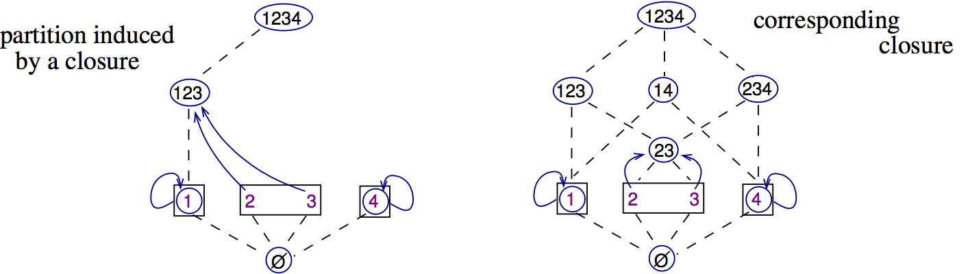
Figure 4: A partitioning closure.

Example 2.3.

Consider the set $S=\{1,2,3,4\}$ and one of its possible partitions $\pi=\{\{1\},\{2,3\},\{4\}\}$. The closure $\eta$ with fix-points $\{\emptyset,\{1\},\{4\},\{1,2,3\},S\}$ induces exactly $\pi$ as a state partition, but the most concrete closure that induces $\pi$ is $\mbox{\sl\small Clo}^{\pi}=\Pi(\eta)={\bigcurlyvee\left(\{\emptyset,\{1\},\{2,3\},\{4\}\},S\right)}$, which is the closure on the right of Figure 4.

Given a partitioning upper closure operator $\rho$, an atom is an element $a$ of $\rho$ such that there does not exists another element $b$ with $\left[\mathbf{bot}\right]\sqsubset b\sqsubset a$. For example, the atoms of $\rho_{\textsc{parSign}}$ are $\left[\mathbf{poseven}\right]$, $\left[\mathbf{posodd}\right]$, $\left[\mathbf{zero}\right]$, $\left[\mathbf{negeven}\right]$, and $\left[\mathbf{negodd}\right]$. In partitioning closures, atoms are all the possible abstractions of singletons: in fact, $\rho_{\textsc{parSign}}(\{n\})$ will never give $\left[\mathbf{pos}\right]$ or $\left[\mathbf{odd}\right]$ since there is always a more precise abstract value describing $n$. In the following, $\textsc{Atom}_{\rho}\left(a\right)$ holds iff $a$ is an atom of $\rho$.

2.4 Abstract semantics

An abstract program semantics is the abstract counterpart of the concrete semantics w.r.t. an abstract program observation: it is meant to compute, for each program point, an abstract state which soundly represents invariant properties of variables at that point. In general, it is computed by an abstract interpreter [Cousot and Cousot (1979)] collecting the set of all the possible values that each variable may have in each program point and abstracting this set in the chosen abstract domain.

Given a concrete program state $\sigma$ and an abstract domain $\rho\in\mbox{\sl uco}(\wp(\mathbb{V}))$, an abstract state ${\sigma^{\rho}}\in{\Sigma^{\rho}}$ is obtained by applying the abstraction $\rho$ to the values of variables stored in it. Namely, ${\sigma^{\rho}}=\langle n^{k_{n}},\mu^{\rho}\rangle$, where $\mu^{\rho}=\langle\varepsilon^{\rho}\rangle$ and $\varepsilon^{\rho}$ is such that $\varepsilon^{\rho}(x)=\rho(\varepsilon(x))$. For simplicity, we can write ${\sigma^{\rho}}(x)=\rho(\sigma(x))$, treating the whole state as a store when applied to variables. In the case of a reference variable $x$, the abstraction ${\sigma^{\rho}}(x)$ gives information about the data structure pointed to by $x$ (e.g., if $\rho=\rho_{\textsc{cyc}}$, the cyclicity of the data structure can be represented). This explains why the heap is not represented explicitly in the abstract state: instead, relevant information about the heap is contained in the abstraction of variables (see the previous discussion before Example 2.2).

In the following, ordering $\leq$ on abstract states is variable-wise comparison between abstract values:

$$\sigma^{\rho}_{1}\leq\sigma^{\rho}_{2}\quad\Leftrightarrow\quad\forall x.\sigma^{\rho}_{1}(x)\subseteq\sigma^{\rho}_{2}(x)$$

The greater an abstract state is, the wider is the set of concrete states it represents. Moreover, a covering of ${\sigma^{\rho}}$ is a set of abstract states $\{\sigma^{\rho}_{1}..\sigma^{\rho}_{n}\}$ such that $\vee_{i}\sigma^{\rho}_{i}={\sigma^{\rho}}$. The set of abstract state trajectories is $\mathbb{T^{\rho}}={\Sigma^{\rho}}^{*}$, namely an abstract trajectory is the computation of a program on the set of abstract states. The trace in $\mathbb{T^{\rho}}$ of a program $P$, starting from the abstract memory $\mu^{\rho}$ is denoted by $\tau^{\mu^{\rho}}_{P}$.

Formally, the abstract program semantics $\mbox{\raisebox{0.0pt}[4.30554pt][4.30554pt]{$\left\llbracket\cdot\right\rrbracket^{\rho}$}}:\mathbb{P}\times{\Sigma_{\iota}^{\rho}}\rightarrow\mathbb{T^{\rho}}$ is such that $\mbox{\raisebox{0.0pt}[4.30554pt][4.30554pt]{$\left\llbracket P\right\rrbracket^{\rho}$}}(S)=\{\tau^{\mu^{\rho}}_{P}~{}|~{}\langle 1^{1},\mu^{\rho}\rangle\in S\}$ is the set of the sequences of abstract states computed starting from the abstract initial states in $S\in\wp({\Sigma_{\iota}^{\rho}})$. We also abuse notation by denoting $\left\llbracket\cdot\right\rrbracket^{\rho}$ also the abstract evaluation of expressions. Namely, $\mbox{\raisebox{0.0pt}[4.30554pt][4.30554pt]{$\left\llbracket\cdot\right\rrbracket^{\rho}$}}:{\mbox{\sc Exp}}\times{\Sigma^{\rho}}\rightarrow\rho(\mathbb{V})$ is such that $\forall x.\>\mbox{\raisebox{0.0pt}[4.30554pt][4.30554pt]{$\left\llbracket e\right\rrbracket^{\rho}$}}({\sigma^{\rho}}(x))=\rho(\left\llbracket e\right\rrbracket({\sigma^{\rho}}(x)))=\rho(\left\llbracket e\right\rrbracket(\rho(\sigma(x))))$. This definition is correct, since by construction, we have that any abstract state ${\sigma^{\rho}}$ corresponds to a set of concrete states, i.e., $\mbox{\raisebox{0.0pt}[4.30554pt][4.30554pt]{${\sigma^{\rho}}=\left\{~{}\overline{\sigma}\in\Sigma~{}\left|\begin{array}[]{l}\overline{\sigma}^{\rho}={\sigma^{\rho}}\end{array}\right.\right\}$}}=\mbox{\raisebox{0.0pt}[4.30554pt][4.30554pt]{$\left\{~{}\overline{\sigma}\in\Sigma~{}\left|\begin{array}[]{l}\forall x\in\mathbb{X}.\>\overline{\sigma}^{\rho}(x)={\sigma^{\rho}}(x)\end{array}\right.\right\}$}}$, namely, it is the set of all the concrete states having as abstraction in $\rho$ precisely ${\sigma^{\rho}}$, and we abuse notation by denoting with $\left\llbracket\cdot\right\rrbracket^{\rho}$ also its additive lift. In other words, $\left\llbracket e\right\rrbracket^{\rho}$ is the best correct approximation of $\left\llbracket e\right\rrbracket$ by means of an abstract value in $\rho$. In general, in order to compute the abstract semantics of a program on an abstract domain $\rho$, we have to equip the domain $\rho$ with the abstract versions of all the operators used for defining expressions. In our language, we should define, for example, the meaning of $+$, $-$, $*$ and $/$ on abstract values, i.e., on sets of concrete values. This is standard in abstract interpretation, and these operations are defined for all the known numerical abstract domains. For instance, the sound approximation of the sum operation on $\rho_{\textsc{par}}$ is the following:

$$\begin{array}[]{ccccl@{\qquad\qquad}ccccl}\left[\mathbf{even}\right]&+&\left[\mathbf{even}\right]&=&\left[\mathbf{even}\right]&\left[\mathbf{top}\right]&+&\_&=&\left[\mathbf{top}\right]\\ \left[\mathbf{even}\right]&+&\left[\mathbf{odd}\right]&=&\left[\mathbf{odd}\right]&\_&+&\left[\mathbf{top}\right]&=&\left[\mathbf{top}\right]\\ \left[\mathbf{odd}\right]&+&\left[\mathbf{even}\right]&=&\left[\mathbf{odd}\right]&\left[\mathbf{bot}\right]&+&\_&=&\left[\mathbf{bot}\right]\\ \left[\mathbf{odd}\right]&+&\left[\mathbf{odd}\right]&=&\left[\mathbf{even}\right]&\_&+&\left[\mathbf{bot}\right]&=&\left[\mathbf{bot}\right]\\ \end{array}$$

We can reason similarly for all the other operators. The use of $\left\llbracket\cdot\right\rrbracket^{\rho}$ in Section 6.2.1 and later in the paper is twofold: (1) to infer invariant properties, as in Example 2.4; and (2) to evaluate expressions at the abstract level.

Example 2.4.

Consider the following code fragment:

⬇

1 i := 10;

2 j := 0;

3 while (i$\geq$0) {

4 i := i-1;

5 j := j+1;

6 }

and an abstraction $\rho=\rho_{\textsc{sign}}$, i.e., the property of interest is the sign of both i and j. By computing the abstract semantics of this simple program, we can observe that inside the loop we lose the sign of i since i starts being positive, but then the ${\mbox{\leavevmode\lstinline{{\lst@@@set@language\lst@@@set@numbers\lst@@@set@frame\lst@@@set@rulecolor\lst@@@set@frame\lst@@@set@numbers\lst@@@set@language\small\rm{\@listingGroup{ltx_lst_identifier}{i}}}}}}-1$ operation makes impossible to know statically the sign of i (the result may be positive, zero or negative starting from i positive or zero), while we have that j always remains positive. Moreover, if the loop terminates we can surely say that, at the end, ${\mbox{\leavevmode\lstinline{{\lst@@@set@language\lst@@@set@numbers\lst@@@set@frame\lst@@@set@rulecolor\lst@@@set@frame\lst@@@set@numbers\lst@@@set@language\small\rm{\@listingGroup{ltx_lst_identifier}{i}}}}}}<0$, namely it is negative (due to the negation of the while guard). Hence, we are able to infer that i is negative and j is positive after line 6. This means that the final abstract state ${\sigma^{\rho}}$ is such that ${{\sigma^{\rho}}(\mbox{$\mbox{\leavevmode\lstinline{{\lst@@@set@language\lst@@@set@numbers\lst@@@set@frame\lst@@@set@rulecolor\lst@@@set@frame\lst@@@set@numbers\lst@@@set@language\small\rm{\@listingGroup{ltx_lst_identifier}{i}}}}}}$})=\left[\mathbf{neg}\right]$ and ${{\sigma^{\rho}}(\mbox{$\mbox{\leavevmode\lstinline{{\lst@@@set@language\lst@@@set@numbers\lst@@@set@frame\lst@@@set@rulecolor\lst@@@set@frame\lst@@@set@numbers\lst@@@set@language\small\rm{\@listingGroup{ltx_lst_identifier}{j}}}}}}$})=\left[\mathbf{pos}\right]$ (in the following, the extensional notation for ${\sigma^{\rho}}$ will be ${{\{\mbox{$\mbox{\leavevmode\lstinline{{\lst@@@set@language\lst@@@set@numbers\lst@@@set@frame\lst@@@set@rulecolor\lst@@@set@frame\lst@@@set@numbers\lst@@@set@language\small\rm{\@listingGroup{ltx_lst_identifier}{i}}}}}}$}\!\leftarrow\!\left[\mathbf{neg}\right],\mbox{$\mbox{\leavevmode\lstinline{{\lst@@@set@language\lst@@@set@numbers\lst@@@set@frame\lst@@@set@rulecolor\lst@@@set@frame\lst@@@set@numbers\lst@@@set@language\small\rm{\@listingGroup{ltx_lst_identifier}{j}}}}}}$}\!\leftarrow\!\left[\mathbf{pos}\right]\}$, similar to the notation for concrete states).

3 Program Slicing

Program slicing [Weiser (1984)] is a program-manipulation technique which extracts from programs those statements which are relevant to a particular portion of a computation. In order to answer the question about which are the relevant statements, an observer needs a window through which only a part of the computation can be seen [Binkley and Gallagher (1996)]. Usually, what identifies the portion of interest in the computation is the value of some set of variables at a certain program point, so that a program slice comes to be the subset (syntactically, in terms of statements) of the original program which contributes directly or indirectly to the values assumed by some set of variables at the program point of interest. The slicing criterion is what specifies the part of the computation which is relevant to the analysis; in this case, a criterion is a pair consisting of a set ${\mathcal{X}}$ of variables and a program point (or line number) $n$. The following definition [Binkley and Gallagher (1996)] is a possible formalization the original idea of program slicing [Weiser (1984)], in the case of a single variable:

Definition 3.1

[Binkley and Gallagher (1996)] For a statement $s$ (at program point $n$) and a variable $x$, the slice $P^{\prime}$ of the program $P$ with respect to the slicing criterion $\langle s,\{x\}\rangle$ is any executable program with the following properties:

1. $P^{\prime}$ can be obtained by deleting zero or more statements from $P$;

2. If $P$ halts on the input $I$, then, each time $s$ is reached in $P$, it is also reached in $P^{\prime}$, and the value of $x$ at $s$ is the same in $P$ and in $P^{\prime}$. If $P$ fails to terminate, then $s$ may be reached more times in $P^{\prime}$ than in $P$, but $P$ and $P^{\prime}$ have the same value for $x$ each time $s$ is executed by $P$.

It is worth noting that Reps and Yang [Reps and Yang (1989)], in their slicing theorem, provide implicitly a similar definition of program slicing, but it only considers terminating computations. The following example provides the intuition of how slicing works.

⬇

1 int c, nl := 0, nw := 0, nc := 0;

2 int in := false;

3 while ((c=getchar())!=EOF) {

4 nc := nc+1;

5 if (c=’ ’ || c=’\n’ || c=’\t’) {

6 in := false; }

7 elseif (in = false) {

8 in := true;

9 nw := nw+1; }

10 if (c = ’\n’) {

11 nl := nl+1; }

12 }

Figure 5: Word-count program.

⬇ 1 int c, nw := 0; 2 int in := false; 3 while ((c=getchar())!=EOF) { 4 5 if (c=’ ’ || c=’\n’ || c=’\t’) { 6 in := false; } 7 elseif (in = false) { 8 in := true; 9 nw := nw+1; } 10 11 }

Figure 6: Slices of the word-count program.

Example 3.2.

Consider the word-count program [Majumdar et al. (2007)] given in Figure 5. It takes in a block of text and outputs the number of lines (nl), words (nw) and characters (nc). Suppose the slicing criterion only cares for the value of nl at the end of the program; then a possible slice is on the left in Figure 6. On the other hand, if the criterion is only interested in nw, then a correct slice is on the right.

Starting from the original definition [Weiser (1984)], the notion of slicing has gone through several generalizations and versions, but one feature is constantly present: the fact that slicing is based on a notion of semantic equivalence that has to hold between a program and its slices or on a corresponding notion of dependency, determining what we keep in the slice while preserving the equivalence relation. What we can observe about definitions of slicing such as the one given in Definition 3.1 is that they are enough precise for finding algorithms for soundly computing slicing, such as [Reps and Yang (1989)], but not enough formal to become suitable to generalizations allowing us to compare different forms of slicing and/or to define new weaker forms of slicing.

In the following, we use the formal framework proposed in [Binkley et al. (2006a)] where several notions and forms of slicing are modeled and compared. This is not the only attempt to provide a formal framework for slicing (see Section 8), but we believe that, due to its semantic-based approach, it is suitable to include an abstraction level to slicing, which can be easily compared with all the other forms of slicing included in the original framework. Hence, in the following section we don’t rewrite a formal framework, but we re-formalize the slicing criterion in order to allow us to easily include abstraction simply as a new parameter. A brief introduction of the formal framework together with some examples showing the differences between the different forms of slicing introduced in the following is given in the Appendix.

3.1 Defining Program Slicing: the formal framework

In this section, our aim is to define the form of slicing that we can lift to an abstract level. Namely, we consider the framework in [Binkley et al. (2006a), Binkley et al. (2006b)], which allows us to define abstract slicing simply by defining an abstract criterion which, independently from the kind of slicing (static, dynamic, conditional, standard, etc.) allows us to observe properties instead of concrete values. Since our aim is to define abstract program slicing as a form of slicing, perfectly integrated in the proposed hierarchy and where the criterion simply has one more parameter describing the abstraction, we need to slightly revise the construction in order to provide a completely unified notation for the slicing criterion. Note that, the present paper will only deal with backward slicing, where the interest is on the part of the program which affects the observation associated with the slicing criterion and not on the part of the program which is affected by such an observation (called instead forward slicing [Tip (1995)]).

Defining slicing criteria

The slicing criterion characterizes what we have to observe of the program in order to decide whether a program is a slice or not of another program. In particular, we have to fix which computations have to be compared, i.e., the inputs and the observations on which the slice and the program have to agree.

In the seminal Weiser approach, given a set of variables of interest ${\mathcal{X}}$ and program statement $s$, here referred by the program point $n$ where $s$ is placed, a slicing criterion was modeled as . In the following, we will gradually enrich and generalize this model in order to include several different notions and forms of slicing. Weiser’s approach is known as static slicing since the equivalence between the original program and the slice has, implicitly, to hold for every possible input. On the other hand, Korel and Laski proposed a new technique called dynamic slicing [Korel and Laski (1988)] which only considers one particular computation, and therefore one particular input, so that the dynamic slice only preserves the (subset of the) meaning of the original program for that input. Hence, in order to characterize a slicing criterion including also dynamic slicing we have to add a parameter describing the set of initial memories ${\mathcal{I}}\subseteq\mathbb{M}$: The criterion is now , where ${\mathcal{I}}=\mathbb{M}$ for static slicing, while ${\mathcal{I}}=\{\mu\}$, with $\mu\in\mathbb{M}$, for dynamic slicing. Finally, Canfora et al. proposed conditioned slicing [Canfora et al. (1998)], which requires that a conditioned slice preserves the meaning of the original program for a set of inputs satisfying one particular condition $\varphi$. Let ${\mathcal{I}}=\left\{~{}\mu\in\mathbb{M}~{}\left|\begin{array}[]{l}\mu\ \mbox{satisfies}\ \varphi\end{array}\right.\right\}$ be the set of input memories satisfying $\varphi$ [Binkley et al. (2006a)]. Hence, the slicing criterion still can be modeled as .

Each type of slicing comes in four forms which differ on what the program and the slices must agree on, namely on the observable semantics that has to agree. In the following, we provide an informal definition of these forms in order to provide the intuition of what will be formally defined afterwards:

Standard

It considers one point in a program with respect to a set of variables. In other words, the standard form of slicing only tracks one program point. Semantically, this form of slicing consists in comparing the program and the slices in terms of the (denotational) I/O semantics from the program inputs selected by the criterion. Namely, for each selected input, the results of the criterion variables in the point of observation must be the same, independently from the executed statements.

Korel and Laski ($\mathtt{KL}$)

It is a stronger form where the program and the slice must follow identical paths [Korel and Laski (1988)]. Semantically, we could say that the program and the slice must have the same (operational) trace semantics w.r.t. the statements kept in the slice, starting from the program inputs selected by the criterion. In other words, as before, the final value must be the same, but in this case these values must be obtained by executing precisely the same statements, i.e., following the same execution path.

Iteration count ($\mathtt{IC}$)

When considering the trace semantics, the same program point inside a loop may be visited more than once, in the following we call $k$-th iteration of a program point $n$ the $k$-th time the program point $n$ is visited. The iteration count form of slicing requires that a program and its slice agree only at a particular $k$-th iteration of a program point of interest. In this way, when a point of interest is inside a loop, we have the possibility to require that the variables must agree only at some iterations of the loop and not always.

Korel and Laski iteration count ($\mathtt{KL}i$)

It is the combination of the last two forms.

In order to deal with these different forms of slicing, the slicing criterion must be enriched with additional information. In particular, the $\mathtt{KL}$ form of slicing does not change where to observe variables, but it does change the observed semantics up to that point. Hence, we simply have to add a boolean parameter $\psi$: true means that we are considering a $\mathtt{KL}$ form and we require that the slice must agree with the program on the execution of statements that are in the slice (and obviously also in the original program); on the other hand, false indicates a standard, non-$\mathtt{KL}$ form of slicing. Hence, a criterion comes to be $({\mathcal{I}},{\mathcal{X}},n,\psi)$.

The $\mathtt{IC}$ form, instead, affects the observation: in order to embed this features in the criterion, the third parameter has to be changed. Let $\{k_{1},..,k_{j}\}\subseteq\mathbb{N}$ be the iterations of the program point $n\in\mathbb{L}$ we are interested in; then, instead of $n$, in the third parameter of the criterion we should have $\langle n,\{k_{1},..,k_{j}\}\rangle$. Therefore, takes the form $({\mathcal{I}},{\mathcal{X}},{\mathcal{O}},\psi)$, where ${\mathcal{O}}\in\mathbb{L}\times\wp(\mathbb{N})$. Note that $\langle n,\mathbb{N}\rangle$ represents the fact that we are interested in all occurrences of $n$, as it happens in the standard form.

There are also some simultaneous ($\mathtt{SIM}$) forms of slicing that consider more than one program point of interest. In order to deal with $\mathtt{SIM}$ forms of slicing, we simply extend the definition of a slicing criterion by considering ${\mathcal{O}}$ as a set instead of a singleton, namely, ${\mathcal{O}}\in\wp(\mathbb{L}\times\wp(\mathbb{N}))$.

In the Appendix there are some simple examples showing the main differences between the several forms of slicing introduced so far.

4 Abstract Program Slicing

In this section we define a weaker notion of slicing based on Abstract Interpretation. In particular, we generalize the formal framework in [Binkley et al. (2006a)] in order to include also the abstract versions of slicing.

Program slicing is used for reducing the size of programs to analyze. Nevertheless, sometimes this reduction is not sufficient for really improving an analysis. Suppose that some variables at some point of execution do not have a desired property (for example, that they are different from $0$, or from null); in order to understand where the error occurred, it would be useful to find those statements which affect such a property of these variables. Standard slicing may return too many statements, making it hard for the programmer to realize which one caused the error.

Example 4.1.

Consider the following program $P$, that inserts a new element elem at position pos in a single-linked list. For simplicity, let pos never exceed the length of list.

⬇

34 y := null;

35 x := list;

36 while (pos>0) {

37 y := x;

38 x := x.next; // by hypothesis, this always succeeds

39 pos := pos-1;

40 }

41 z := new Node(elem);

42 z.next := x;

43 if (y = null) {

44 list := z;

45 } else {

46 y.next = z;

47 }

Suppose that list is cyclic after line 47, i.e., a traversal of the list visits the same node twice. A close inspection of the code reveals that no cycle is created between lines 34 and 47: list is cyclic after line 47 if and only if it was cyclic before line 34.

In the standard approach, it is possible to set the value of list after line 47 as the slicing criterion. In this case, since list can be modified at lines 41–47, at least this piece of code must be included in the slice.

On the other hand, let the cyclicity of list after line 47 be the property of interest, represented by $\rho_{\textsc{cyc}}$ (Example 2.2). Since this property of list does not change, the entire code can be removed from the slice.

4.1 Defining Abstract Program Slicing

We introduce abstract program slicing, which compares a program and its abstract slices by considering properties instead of exact values of program variables. Such properties are represented as abstract domains, based on the theory of Abstract Interpretation (Section 2.2).

We first introduce the notion of abstract slicing criterion, where the property of interest is also specified. For the sake of simplicity, the definition only refers to non-$\mathtt{SIM}$ forms (i.e., ${\mathcal{O}}$ is a singleton instead of a set of occurrences: ${\mathcal{O}}\in\mathbb{L}\times\wp(\mathbb{N})$). In order to make abstract the criterion we have to formalize in it the properties that we aim at observing on program variables. In particular we could think of observing different properties for different variables. Hence, we define a criterion abstraction ${\mathcal{A}}$ defined as a tuple of abstract domains, each one relative to a specific subset of program variables: Let ${\mathcal{X}}$ be a set of variables of interest in $P$ and $\{X_{i}\}_{i\in[1,k]}\subseteq\wp({\mathcal{X}})$ a partition of ${\mathcal{X}}$, the notation ${\mathcal{A}}=\langle X_{1}:\rho_{1},..,X_{k}:\rho_{k}\rangle$ means that each uco $\rho_{i}$ is applied to the set of variable $X_{i}$ (left implicit when it is clear from the context), meaning that $\rho_{i}$ is precisely the property to observe on $X_{i}$. In the following, we denote by ${\mathcal{A}}_{|X_{i}}$ the property observed on $X_{i}$, formally ${\mathcal{A}}_{|X_{i}}=\rho_{i}$. This is the most general representation, accounting also for relational domains. When ucos will be applied to singletons, the notation will be simplified ($x:\rho$ instead of $\{x\}:\rho$).

Example 4.2.

Let $x$, $y$, $z$ and $w$ be the variables in ${\mathcal{X}}$. Let ${\mathcal{A}}$ be $\langle x:\rho_{\textsc{par}},\{y,z\}:\rho_{\textsc{int}}^{+},w:\rho_{\textsc{sign}}\rangle$, meaning that the interest is on the parity of $x$, the sign of $w$, and the (relational) property of intervals [Cousot and Cousot (1979)] of the value $x+y$. When abstracting a criterion w.r.t. ${\mathcal{A}}$, the required observation at a program state $\sigma$ is

$$\rho_{\textsc{par}}(\sigma(x))\qquad\rho_{\textsc{int}}^{+}(\sigma(y)+\sigma(z))\qquad\rho_{\textsc{sign}}(\sigma(w))$$

In order to be as general as possible, we consider relational properties of variables (see Section 2), so that properties are associated with tuples instead of single variables. In this case, a property is said to involve some set (tuple) of variables. Given a memory $\mu$, $\rho(\mu)$ is the result of applying $\rho$ to the values in $\mu$ of the variables involved by the abstract domain, and ${\mathcal{A}}(\mu)$ is the corresponding notion for tuples of ucos.

Definition 4.3 (Abstract criterion)

Let ${\mathcal{I}}\subseteq\mathbb{M}$ be a set of input memories, ${\mathcal{X}}\subseteq\mathbb{X}$ be a set of variables of interest; ${\mathcal{O}}\in\mathbb{L}\times\wp(\mathbb{N})$ be a set of occurrences of interest; $\psi$ be a truth value indicating if the slicing is in $\mathtt{KL}$ form. Moreover, let ${\mathcal{X}}$ be the set of variables of interest and ${\mathcal{A}}\mbox{\raisebox{0.0pt}[4.30554pt][4.30554pt]{$\stackrel{{\scriptstyle\mbox{\tiny def}}}{{\;=\;}}$}}\langle X_{1}:\rho_{1},\ldots,X_{k}:\rho_{k}\rangle$, with $\{X_{i}\}_{i\in[1,k]}$ a partition of ${\mathcal{X}}$. Then, the abstract slicing criterion is ,

Note that, when dealing with non-abstract notions of slicing, we have that each domains is the identity on each single variable, namely ${\mathcal{A}}=\langle x_{1}:\rho_{\textsc{id}},\ldots,x_{k}:\rho_{\textsc{id}}\rangle$, where $\rho_{\textsc{id}}\mbox{\raisebox{0.0pt}[4.30554pt][4.30554pt]{$\stackrel{{\scriptstyle\mbox{\tiny def}}}{{\;=\;}}$}}\lambda x.x$. It is also worth pointing out that, exactly as it happens for non-abstract forms, ${\mathcal{I}}=\mathbb{M}$ corresponds to static slicing, and $|{\mathcal{I}}|=1$ corresponds to dynamic slicing; in the intermediate cases, we have conditioned slicing.

4.2 The extended formal framework

In this section, we extend a formal framework in which all forms of abstract slicing can be formally represented. It is an extension of the mathematical structure introduced by Binkley. Following their framework, we represent a form of abstract slicing by a pair $(\sqsubseteq,{\mathcal{E}}_{{\mathcal{A}}})$, where $\sqsubseteq$ is the traditional syntactic ordering, and ${\mathcal{E}}_{{\mathcal{A}}}$ is a function mapping abstract slicing criteria to semantic equivalence relations on programs. Given two programs $P$ and $Q$, and an abstract slicing criterion , we say that $Q$ is a $(\sqsubseteq,{\mathcal{E}}_{{\mathcal{A}}})$-(abstract)-slice of $P$ with respect to iff $Q\sqsubseteq P$ and $\langle P,Q\rangle\in{\mathcal{E}}_{{\mathcal{A}}}($ (i.e., $P$ and $Q$ are equivalent w.r.t. ${\mathcal{E}}_{{\mathcal{A}}}$). Some preliminary notions are needed to define ${\mathcal{E}}_{{\mathcal{A}}}$ in the context of abstract slicing.

An abstract memory w.r.t. a set of variables of interests ${\mathcal{X}}$ (partitioned in $\{X_{i}\}_{i\in[1,k]}$) is obtained from a memory by restricting its domain to the variables of interest, and assigning to each set $X_{i}$ of variables an abstract value determined by the corresponding abstract property of interest $\rho_{i}$.

Definition 4.4

Let $\mu\!\in\!\mathbb{M}$ be a memory, ${\mathcal{X}}$ be the set of a tuple of sets of variables of interest, and ${\mathcal{A}}=\langle X_{1}:\rho_{1},\ldots,X_{k}:\rho_{k}\rangle$ be the corresponding tuple of properties of interest such that $\{X_{i}\}_{i\in[1,k]}$ is a partition of ${\mathcal{X}}$. The abstract restriction of a memory $\mu$ w.r.t. the state abstraction ${\mathcal{A}}$ is defined as $\mu\upharpoonright^{\alpha}_{{\mathcal{A}}}{\mathcal{X}}\mbox{\raisebox{0.0pt}[4.30554pt][4.30554pt]{$\stackrel{{\scriptstyle\mbox{\tiny def}}}{{\;=\;}}$}}{\mathcal{A}}\circ\mu({\mathcal{X}})\mbox{\raisebox{0.0pt}[4.30554pt][4.30554pt]{$\stackrel{{\scriptstyle\mbox{\tiny def}}}{{\;=\;}}$}}\langle\rho_{1}(\mu(X_{1})),\ldots,\rho_{k}(\mu(X_{k}))\rangle$.

Example 4.5.

Let $\mathbb{X}=\{x_{1},x_{2},x_{3},x_{4}\}$ be a set of variables, and suppose that the properties of interest are the (relational) sign of the product $x_{1}x_{2}$ and the parity of $x_{3}$ (both defined in Section 2). We slightly abuse notation by denoting as $\rho_{\textsc{sign}}$ also its extension to pairs $(v,t)$ where the sign of their product matters: e.g., $\rho_{\textsc{sign}}(3,-5)=(\left[\mathbf{neg}\right])$. In our formal framework, ${\mathcal{A}}$ is defined as $\langle\{x_{1},x_{2}\}:\rho_{\textsc{sign}},x_{3}:\rho_{\textsc{par}}\rangle$. Let $\mu(x_{1})=1$, $\mu(x_{2})=2$, $\mu(x_{3})=3$, and $\mu(x_{4})=4$; then, $\mu\upharpoonright^{\alpha}_{{\mathcal{A}}}{\mathcal{X}}$ comes to be ${\mathcal{A}}\circ\mu({\mathcal{X}})=\langle\left[\mathbf{pos}\right],\left[\mathbf{odd}\right]\rangle$.

The abstract projection operator modifies a state trajectory by removing all those states which do not contain occurrences or points of interest. If there is a state that contains an occurrence of interest, then its memory state is restricted via $\upharpoonright^{\alpha}$ to the variables of interest, and only a property is considered for each tuple. In the following, the abstract projection $\mathit{Proj}^{\alpha}$ is formally defined.

Definition 4.6 (Abstract Projection)

Let , and ${\mathcal{L}}\subseteq\mathbb{L}$ such that ${\mathcal{L}}\neq\emptyset$ if $\psi=\mbox{\sl true}$, ${\mathcal{L}}=\emptyset$ otherwise. For any $n\in\mathbb{L}$, $k\in\mathbb{N}$, $\mu\in\mathbb{M}$, we define a function $\mathit{Proj}^{0\alpha}$ as:

$$\mathit{Proj}^{0\alpha}_{({\mathcal{X}},{\mathcal{O}},{\mathcal{L}},{\mathcal{A}})}(n^{k},\mu)\mbox{\raisebox{0.0pt}[4.30554pt][4.30554pt]{$\stackrel{{\scriptstyle\mbox{\tiny def}}}{{\;=\;}}$}}\left\{\begin{array}[]{l l}\langle n^{k},\mu\upharpoonright^{\alpha}_{{\mathcal{A}}}{\mathcal{X}}\rangle&\mbox{if }\exists\langle n,K\rangle\in{\mathcal{O}}.\>k\in K\\ \langle n^{k},\bot\rangle&\mbox{if }\nexists(n,K)\in{\mathcal{O}}.\>k\in K\mbox{ and }n\in{\mathcal{L}}\\ \varepsilon&\mbox{otherwise}\end{array}\right.$$

The abstract projection $\mathit{Proj}^{\alpha}$ is the extension of $\mathit{Proj}^{0\alpha}$ to sequences:

$$\begin{array}[]{l}\mathit{Proj}_{({\mathcal{X}},{\mathcal{O}},{\mathcal{L}},{\mathcal{A}})}^{\alpha}(\langle(n_{1}^{k_{1}},\mu_{1})\ldots(n_{l}^{k_{l}},\mu_{l})\rangle)=\\ \qquad\qquad\qquad\mathit{Proj}^{0\alpha}_{({\mathcal{X}},{\mathcal{O}},{\mathcal{L}},{\mathcal{A}})}(n_{1}^{k_{1}},\mu_{1})\circ\ldots\circ{\mathit{Proj}^{0\alpha}}_{({\mathcal{X}},{\mathcal{O}},{\mathcal{L}},{\mathcal{A}})}(n_{l}^{k_{l}},\mu_{l})\end{array}$$

$\mathit{Proj}^{0\alpha}$ takes a state from a state trajectory, and returns either one pair or an empty sequence $\varepsilon$. Abstract projection allows us to define all the semantic equivalence relations we need for representing the abstract forms of slicing.

Example 4.7.

Consider the program $P$ in Figure 7.

⬇ 1 read(n); 2 i := 1; 3 s := 0; 4 5 while (i <= n) { 6 s := s+i; 7 8 i := i+1; } 9 write(i,n,s);
Program $P$	Program $Q$

Figure 7: Program $P$ and its slice.

Consider ${\mathcal{I}}=\mathbb{M}$ (meaning that we are considering static slicing), ${{{\mathcal{X}}=\{\mbox{\leavevmode\lstinline{{\lst@@@set@language\lst@@@set@numbers\lst@@@set@frame\lst@@@set@rulecolor\lst@@@set@frame\lst@@@set@numbers\lst@@@set@language\small\rm{\@listingGroup{ltx_lst_identifier}{i}}}}}},\mbox{\leavevmode\lstinline{{\lst@@@set@language\lst@@@set@numbers\lst@@@set@frame\lst@@@set@rulecolor\lst@@@set@frame\lst@@@set@numbers\lst@@@set@language\small\rm{\@listingGroup{ltx_lst_identifier}{s}}}}}}\}$, ${\mathcal{O}}=\langle 8,\mathbb{N}\rangle$ (meaning that we check the value of variables of interest at each iteration of program point $8$). Moreover, we consider ${{{\mathcal{A}}=\langle\mbox{$\mbox{\leavevmode\lstinline{{\lst@@@set@language\lst@@@set@numbers\lst@@@set@frame\lst@@@set@rulecolor\lst@@@set@frame\lst@@@set@numbers\lst@@@set@language\small\rm{\@listingGroup{ltx_lst_identifier}{i}}}}}}$}:\rho_{\textsc{sign}},\mbox{$\mbox{\leavevmode\lstinline{{\lst@@@set@language\lst@@@set@numbers\lst@@@set@frame\lst@@@set@rulecolor\lst@@@set@frame\lst@@@set@numbers\lst@@@set@language\small\rm{\@listingGroup{ltx_lst_identifier}{s}}}}}}$}:\rho_{\textsc{par}}\rangle$. Then in Figure 8 we have the corresponding abstract projection (the concrete trace is given in the Appendix, Example 24). In this figure, we depict states as set of boxes, the first one contains the number of the executed program point (with the iteration counter as apex), while the other boxes are the different variables associations. The cross on a box means that the projection does not consider that variable or state. So for instance, in this example we care only of states $6^{i}$ and $8^{i}$, and in particular, in states $6^{i}$ we are not interested in the values of variables, while in states $8^{i}$ we are interested in the sign of $i$ and in the parity of $s$ (if we would be interested in the value of these variables we would have the value instead of their property, as it happens in the examples in the Appendix).

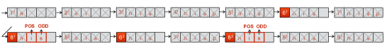
Figure 8: Abstract trajectory projection for program $P$ in Example 4.7

4.3 Abstract Unified Equivalence

The only missing step for completing the formal definition of abstract slicing in the formal framework is to characterize the functions mapping abstract slicing criteria to abstract semantic equivalence relations.

Definition 4.8 (Abstract Unifying Equivalence)

Let $P$ and $Q$ be executable programs, and be an abstract criterion. Then $P$ is abstract-equivalent to $Q$ if and only if, for every $\mu\in{\mathcal{I}}$, it holds that $\mathit{Proj}^{\alpha}_{({\mathcal{X}},{\mathcal{O}},{\mathcal{L}},{\mathcal{A}})}(\tau_{P}^{\mu})=\mathit{Proj}^{\alpha}_{({\mathcal{X}},{\mathcal{O}},{\mathcal{L}},{\mathcal{A}})}(\tau_{Q}^{\mu})$, where ${\mathcal{L}}=\mathbb{L}_{P}\cap\mathbb{L}_{Q}$ if $\psi=\mbox{\sl true}$. The function ${\mathcal{E}}_{\mathcal{A}}$ maps each criterion to a corresponding abstract semantic equivalence relation.

Therefore, a generic form of slicing can be represented as $(\sqsubseteq,{\mathcal{E}}_{{\mathcal{A}}})$. This can be used to formally define both traditional and abstract forms of slicing in the presented abstract formal framework, so that the latter comes to be a generalization of the original formal framework. The following examples show how it is possible to use these definitions in order to check whether a program is an abstract slice of another one.

⬇ 1 read(n); 2 read(s); 3 4 write(n,s);

Figure 9: Programs $P$ and $Q$

Example 4.9.

Consider the programs $P$ and $Q$ in Figure 9. Let , meaning that we are interested in the parity of s (${{\mathcal{A}}=\langle\mbox{$\mbox{\leavevmode\lstinline{{\lst@@@set@language\lst@@@set@numbers\lst@@@set@frame\lst@@@set@rulecolor\lst@@@set@frame\lst@@@set@numbers\lst@@@set@language\small\rm{\@listingGroup{ltx_lst_identifier}{s}}}}}}$}:\rho_{\textsc{par}}\rangle$) at the end of execution (${\mathcal{O}}=\{\langle 7,\mathbb{N}\rangle\}$) for all possible inputs (${\mathcal{I}}=\mathbb{M}$), in non-$\mathtt{KL}$ form. Since $Q\sqsubseteq P$, in order to show that $Q$ is an abstract static slice of $P$ with respect to , we have to show that $\langle P,Q\rangle\in{\mathcal{E}}_{{\mathcal{A}}}($ holds. Let $\mu=\{n\!\leftarrow\!a,s\!\leftarrow\!b\}$ for some $a,b\in\mathbb{N}$ be an initial memory. The trajectory of $P$ from $\mu$ contains the following steps of computation:

Applying $\mathit{Proj}^{\alpha}$ (with ${\mathcal{L}}=\emptyset$ since $\psi=\mbox{\sl false}$) to $\tau_{P}^{\mu}$ returns only the abstract value of the variable s at point $7$ (due to ):

$$\begin{array}[]{rcl}\mathit{Proj}^{\alpha}_{({\mathcal{X}},{\mathcal{O}},\emptyset,{\mathcal{A}})}(\tau_{P}^{\mu})&=&\langle 7^{1},\{n\!\leftarrow\!a,s\!\leftarrow\!b{+}a(a{+}1),i\!\leftarrow\!a{+}1\}\upharpoonright^{\alpha}_{{\mathcal{A}}}\{\langle s\rangle\})\rangle\\ &=&\langle 7^{1},\rho_{\textsc{par}}(b{+}a(a{+}1))\rangle=\langle 7^{1},\rho_{\textsc{par}}(b)\rangle\end{array}$$

Since we have $7^{1}\!=\!\langle 7,1\rangle\!\in\!{\mathcal{O}}$, $\mathit{Proj}^{0\alpha}_{({\mathcal{X}},{\mathcal{O}},\emptyset,{\mathcal{A}})}(7^{1},\{n\!\leftarrow\!a,s\!\leftarrow\!b{+}a(a{+}1),i\!\leftarrow\!a{+}1\})$ returns $\langle 7^{1},\mu\upharpoonright^{\alpha}_{{\mathcal{A}}}{\mathcal{X}}\rangle=\langle 7^{1},\{n\!\leftarrow\!a,s\!\leftarrow\!b{+}a(a{+}1),i\!\leftarrow\!a{+}1\}\upharpoonright^{\alpha}_{{\mathcal{A}}}\{\langle s\rangle\}\rangle$. The abstract memory restricts the domain of $\mu$ to variables of interest, so we consider only the part of $\mu$ regarding $s$, i.e., $b\!+\!a(a\!+\!1)$. Hence, we have $\langle 7^{1},\rho_{\textsc{par}}(\langle b\!+\!a(a\!+\!1)\rangle)\rangle$. Since the parity of $b{+}a(a{+}1)$ only depends on the parity of $b$, being either $a$ or $a+1$ even, the final result is $\langle 7^{1},\rho_{\textsc{par}}(b)\rangle$. Consider now the execution of $Q$ from $\mu$, which corresponds to the following state trajectory:

Applying $\mathit{Proj}^{\alpha}$ to $\tau_{Q}^{\mu}$ gives:

$$\begin{array}[]{rcl}\mathit{Proj}^{\alpha}_{({\mathcal{X}},{\mathcal{O}},\emptyset,{\mathcal{A}})}(\tau_{Q}^{\mu})=\langle 7^{1},\{n\!\leftarrow\!a,s\!\leftarrow\!b\}\upharpoonright^{\alpha}_{{\mathcal{A}}}\{\langle s\rangle\}\rangle=\langle 7^{1},\rho_{\textsc{par}}(b)\rangle\end{array}$$

Therefore, $\mathit{Proj}^{\alpha}_{({\mathcal{X}},{\mathcal{O}},\emptyset,{\mathcal{A}})}(\tau_{P}^{\mu})$ is equal to $\mathit{Proj}^{\alpha}_{({\mathcal{X}},{\mathcal{O}},\emptyset,{\mathcal{A}})}(\tau_{Q}^{\mu})$. As $\mu$ is an arbitrary input, this equation holds for each $\mu\in\mathbb{M}$, so that $\langle P,Q\rangle\in{\mathcal{E}}_{{\mathcal{A}}}($, and this implies that $Q$ is an abstract static slice of $P$ w.r.t. .

⬇ 1 read(n); 2 s := 0; 3 4 write(n,s);

Figure 10: Programs $R$ and $S$

Example 4.10.

Consider the programs $R$ and $S$ in Figure 10, and let be ${{({\mathcal{I}},\{\mbox{$\mbox{\leavevmode\lstinline{{\lst@@@set@language\lst@@@set@numbers\lst@@@set@frame\lst@@@set@rulecolor\lst@@@set@frame\lst@@@set@numbers\lst@@@set@language\small\rm{\@listingGroup{ltx_lst_identifier}{s}}}}}}$}\},\{\langle 7,\mathbb{N}\rangle\},\mbox{\sl false},\langle\mbox{\leavevmode\lstinline{{\lst@@@set@language\lst@@@set@numbers\lst@@@set@frame\lst@@@set@rulecolor\lst@@@set@frame\lst@@@set@numbers\lst@@@set@language\small\rm{\@listingGroup{ltx_lst_identifier}{s}}}}}}:\rho_{\textsc{par}}\rangle)$, where ${{\mathcal{I}}=\{~{}\mu\mid\mu(\mbox{$\mbox{\leavevmode\lstinline{{\lst@@@set@language\lst@@@set@numbers\lst@@@set@frame\lst@@@set@rulecolor\lst@@@set@frame\lst@@@set@numbers\lst@@@set@language\small\rm{\@listingGroup{ltx_lst_identifier}{n}}}}}}$})\!\in\!4\mathbb{Z}~{}\}$; i.e., we are interested in the parity of s at the end of the execution for all inputs where n is a multiple of $4$. Since $S{\sqsubseteq}R$, in order to show that $S$ is an abstract conditioned slice of $R$ w.r.t. , we have to show that $\langle R,S\rangle\in{\mathcal{E}}_{{\mathcal{A}}}($ holds, namely that they have the same abstract projection. Let $\mu\in{\mathcal{I}}$ be an initial memory, and suppose ${\mu(\mbox{$\mbox{\leavevmode\lstinline{{\lst@@@set@language\lst@@@set@numbers\lst@@@set@frame\lst@@@set@rulecolor\lst@@@set@frame\lst@@@set@numbers\lst@@@set@language\small\rm{\@listingGroup{ltx_lst_identifier}{n}}}}}}$})=a=4m$. The trajectory $\tau_{R}^{\mu}$ of $R$ from $\mu$ contains the following computations:

While executing $S$ from $\mu$ gives the state trajectory $\tau_{S}^{\mu}$

Applying $\mathit{Proj}^{\alpha}$ to both state trajectories we have:

$$\begin{array}[]{rcl}\mathit{Proj}^{\alpha}_{({\mathcal{X}},{\mathcal{O}},\emptyset,{\mathcal{A}})}(\tau_{R}^{\mu})&=&\langle 7^{1},\{n\!\leftarrow\!a,s\!\leftarrow\!a(a{+}1)/2,i\!\leftarrow\!a{+}1\}\upharpoonright^{\alpha}_{{\mathcal{A}}}\langle\{s\}\rangle\rangle=\langle 7^{1},\rho_{\textsc{par}}(a(a\!+\!1)/2)\rangle\\ &=&\langle 7^{1},\rho_{\textsc{par}}(2m(4m{+}1))\rangle=\langle 7^{1},2\mathbb{Z}\rangle\\ &=&\langle 7^{1},\rho_{\textsc{par}}(0)\rangle=\langle 7^{1},\{n\!\leftarrow\!a,s\!\leftarrow\!0\}\upharpoonright^{\alpha}_{{\mathcal{A}}}\langle\{s\}\rangle\rangle=\mathit{Proj}^{\alpha}_{({\mathcal{X}},{\mathcal{O}},\emptyset,{\mathcal{A}})}(\tau_{S}^{\mu})\end{array}$$

Therefore, we have $\mathit{Proj}^{\alpha}_{({\mathcal{X}},{\mathcal{O}},\emptyset,{\mathcal{A}})}(\tau_{R}^{\mu})=\mathit{Proj}^{\alpha}_{({\mathcal{X}},{\mathcal{O}},\emptyset,{\mathcal{A}})}(\tau_{S}^{\mu})$ . As $\mu$ is an arbitrary input from ${\mathcal{I}}$, this equation holds for each $\mu\in{\mathcal{I}}$, so that $\langle R,S\rangle\in{\mathcal{E}}_{{\mathcal{A}}}($, and this implies that $S$ is an abstract conditioned slice of $R$ w.r.t. . It is worth noting, that $S$ is not a static abstract slice of $R$ since for all the input values $a\notin 4\mathbb{Z}$ for $n$ the parity of the final value of s is not necessarily even.

4.4 Comparing forms of Abstract Slicing

This section provides a formal theory allowing us to compare abstract forms of slicing between themselves, and with non-abstract ones. First of all, we show under which conditions an abstract semantic equivalence relation subsumes another one; analogously, we show when the form of (abstract) slicing, corresponding to the former equivalence relation, subsumes the form of (abstract) slicing corresponding to the latter one. Such results are necessary in order to obtain a precise characterization of the extension of the weaker than relation (whose original definition is recalled in the Appendix) to the abstract forms of slicing.

The following lemma shows under which conditions on the slicing criteria there is a relation of subsumption between two semantic equivalence relations. In the following, we denote $\overline{\sqsubseteq}$ the relation "more concrete than" in the lattice of abstract interpretations between tuples of abstractions. Formally, let us consider ${\mathcal{A}}^{1}=\langle X_{1}^{1}:\rho_{1}^{1},\ldots,X_{k^{1}}^{1}:\rho_{k^{1}}^{1}\rangle$ defined on the variables ${\mathcal{X}}^{1}$ and ${\mathcal{A}}^{2}=\langle X_{1}^{2}:\rho_{1}^{2},\ldots,X_{k^{2}}^{2}:\rho_{k^{2}}^{2}\rangle$ defined on the variables ${\mathcal{X}}^{2}$, such that ${\mathcal{X}}^{1}\subseteq{\mathcal{X}}^{2}$, $k^{1}\leq k^{2}$ and $\forall i\leq k^{1}$ we have $X^{1}_{i}=X^{2}_{i}$, namely the variables in common are partitioned in the same way. Then ${\mathcal{A}}^{2}\overline{\sqsubseteq}{\mathcal{A}}^{1}$ iff $\forall X_{i}\in{\mathcal{X}}^{1}.\>\rho_{i}^{2}\sqsubseteq\rho^{1}_{i}$. Note that, for all the variables in ${\mathcal{X}}^{2}\smallsetminus{\mathcal{X}}^{1}$, the abstraction ${\mathcal{A}}^{1}$ does not require any particular observation, hence on these variables surely ${\mathcal{A}}^{2}$ is more precise. The following relation is such that, when both ${\mathcal{A}}^{1}$ and ${\mathcal{A}}^{2}$ are the identity on all the variables of interest, then the resulting criterion relation is the same proposed in [Binkley et al. (2006b)] (see the Appendix for details) for characterizing the original formal framework.

Lemma 4.11.

Let two abstract slicing criteria and be given. If (1) ${\mathcal{I}}^{1}\subseteq{\mathcal{I}}^{2}$; (2) ${\mathcal{O}}^{1}\subseteq{\mathcal{O}}^{2}$; (3) ${\mathcal{X}}^{1}\subseteq{\mathcal{X}}^{2}$; (4) $\psi^{1}\Rightarrow\psi^{2}$; and (5) ${\mathcal{A}}^{2}\overline{\sqsubseteq}{\mathcal{A}}^{1}$ (denoted ), then $(\sqsubseteq,{\mathcal{E}}($ subsumes $(\sqsubseteq,{\mathcal{E}}($, i.e., for every $P$ and $Q$ such that $Q\sqsubseteq P$, $\langle P,Q\rangle\in{\mathcal{E}}($ implies $\langle P,Q\rangle\in{\mathcal{E}}($.

Proof 4.12.

First of all, note that, if ${\mathcal{A}}^{1}={\mathcal{A}}^{2}=\rho_{\mbox{\sl\tiny id}}$, namely if we are considering concrete criteria, then $\rightarrow_{\mbox{\tiny${\mathcal{A}}$}}$ collapses to the concrete relation defined in [Binkley et al. (2006a)] (which is the $\rightarrow$ defined in Equation 2 in the Appendix). Hence, in this case, the results holds by [Binkley et al. (2006a)].
Suppose $\langle P,Q\rangle\in{\mathcal{E}}($ with $Q\sqsubseteq P$, namely $Q$ slice of $P$ w.r.t. ${\mathcal{E}}($. This means that, for each $\mu_{0}\in{\mathcal{I}}^{2}$ $\mathit{Proj}^{\alpha}_{({\mathcal{X}}^{2},{\mathcal{O}}^{2},{\mathcal{L}}^{2},{\mathcal{A}}^{2})}(\tau_{P}^{\mu_{0}})=\mathit{Proj}^{\alpha}_{({\mathcal{X}}^{2},{\mathcal{O}}^{2},{\mathcal{L}}^{2},{\mathcal{A}}^{2})}(\tau_{Q}^{\mu_{0}})$, where ${\mathcal{L}}^{2}$ is defined as in Definition 4.8. This means that, for each state $\langle n^{k},\mu\rangle$ in the trajectory $\tau_{P}^{\mu_{0}}$, whose projection $\mathit{Proj}^{0\alpha}_{({\mathcal{X}}^{2},{\mathcal{O}}^{2},{\mathcal{L}}^{2},{\mathcal{A}}^{2})}(n^{k},\mu)_{P}$ is not empty, there exists a state $\langle n^{k},\mu^{\prime}\rangle$ in $\tau_{Q}^{\mu_{0}}$ with the same projection. Let us consider now, $\mu\in{\mathcal{I}}^{1}\subseteq{\mathcal{I}}^{2}$. We prove that on these states $\mathit{Proj}^{0\alpha}_{({\mathcal{X}}^{1},{\mathcal{O}}^{1},{\mathcal{L}}^{1},{\mathcal{A}}^{1})}(n^{k},\mu)=\mathit{Proj}^{0\alpha}_{({\mathcal{X}}^{2},{\mathcal{O}}^{2},{\mathcal{L}}^{2},{\mathcal{A}}^{2})}(n^{k},\mu)$ (and in this case there is a corresponding state in the trajectory of $Q$), or it is empty (and in this case also the state in $Q$ has empty projection). Recall that

$$\mathit{Proj}^{0\alpha}_{({\mathcal{X}}^{1},{\mathcal{O}}^{1},{\mathcal{L}}^{1},{\mathcal{A}}^{1})}(n^{k},\mu)\mbox{\raisebox{0.0pt}[4.30554pt][4.30554pt]{$\stackrel{{\scriptstyle\mbox{\tiny def}}}{{\;=\;}}$}}\left\{\begin{array}[]{l l}\langle n^{k},\mu\upharpoonright^{\alpha}_{{\mathcal{A}}^{1}}{\mathcal{X}}^{1}\rangle&\mbox{if }\exists\langle n,K\rangle\in{\mathcal{O}}^{1}.\>k\in K\\ \langle n^{k},\bot\rangle&\mbox{if }\nexists(n,K)\in{\mathcal{O}}^{1}.\>k\in K\mbox{ and }n\in{\mathcal{L}}^{1}\\ \varepsilon&\mbox{otherwise}\end{array}\right.$$

where also ${\mathcal{L}}^{1}$ is defined as in Definition 4.8. Note that, since we are considering both the criteria on the same pair of programs, we have also that $\psi^{1}\Rightarrow\psi^{2}$ corresponds to saying that ${\mathcal{L}}^{1}\subseteq{\mathcal{L}}^{2}$. At this point

• If $\mathit{Proj}^{0\alpha}_{({\mathcal{X}}^{1},{\mathcal{O}}^{1},{\mathcal{L}}^{1},{\mathcal{A}}^{1})}(n^{k},\mu)_{P}=\langle n^{k},\mu\upharpoonright^{\alpha}_{{\mathcal{A}}^{1}}{\mathcal{X}}^{1}\rangle$ then $\exists\langle n,K\rangle\in{\mathcal{O}}^{1}.\>k\in K$, but ${\mathcal{O}}^{1}\subseteq{\mathcal{O}}^{2}$, hence $\langle n,K\rangle\in{\mathcal{O}}^{2}.\>k\in K$. This mean that $\mathit{Proj}^{0\alpha}_{({\mathcal{X}}^{2},{\mathcal{O}}^{2},{\mathcal{L}}^{2},{\mathcal{A}}^{2})}(n^{k},\mu)_{P}=\langle n^{k},\mu\upharpoonright^{\alpha}_{{\mathcal{A}}^{2}}{\mathcal{X}}^{2}\rangle$, which by hypothesis is equal to $\mathit{Proj}^{0\alpha}_{({\mathcal{X}}^{2},{\mathcal{O}}^{2},{\mathcal{L}}^{2},{\mathcal{A}}^{2})}(n^{k},\mu^{\prime})_{Q}$, for a memory $\mu^{\prime}$. By definition and hypothesis, $\mu\upharpoonright^{\alpha}_{{\mathcal{A}}^{2}}{\mathcal{X}}^{2}={\mathcal{A}}^{2}\circ\mu({\mathcal{X}})={\mathcal{A}}^{2}\circ\mu^{\prime}({\mathcal{X}})$. Namely, $\langle\rho_{1}^{2}(\mu(X_{1})),\ldots,\rho_{k^{2}}^{2}(\mu(X_{k^{2}}))\rangle=\langle\rho_{1}^{2}(\mu^{\prime}(X_{1})),\ldots,\rho_{k^{2}}^{2}(\mu^{\prime}(X_{k^{2}}))\rangle$. Therefore, in particular, $\forall i\in[1,k^{1}]\subseteq[1,k^{2}]$ we have $\rho_{i}^{2}(\mu(X_{i}))=\rho_{i}^{2}(\mu^{\prime}(X_{i}))$, but by hypothesis $\rho^{2}_{i}\sqsubseteq\rho^{1}_{i}$, hence we also have $\rho_{i}^{1}(\mu(X_{i}))=\rho_{i}^{1}(\mu^{\prime}(X_{i}))$ (by properties of ucos). But then $\langle\rho_{1}^{1}(\mu(X_{1})),\ldots,\rho_{k^{1}}^{1}(\mu(X_{k^{1}}))\rangle=\langle\rho_{1}^{1}(\mu^{\prime}(X_{1})),\ldots,\rho_{k^{1}}^{1}(\mu^{\prime}(X_{k^{1}}))\rangle$, namely ${\mathcal{A}}^{1}\circ\mu({\mathcal{X}})={\mathcal{A}}^{1}\circ\mu^{\prime}({\mathcal{X}})$. Hence

  $$\begin{array}[]{lll}\mathit{Proj}^{0\alpha}_{({\mathcal{X}}^{1},{\mathcal{O}}^{1},{\mathcal{L}}^{1},{\mathcal{A}}^{1})}(n^{k},\mu)_{P}&=&\langle n^{k},\mu\upharpoonright^{\alpha}_{{\mathcal{A}}^{1}}{\mathcal{X}}^{1}\rangle\\ &=&\langle n^{k},{\mathcal{A}}^{1}\circ\mu({\mathcal{X}})\rangle=\langle n^{k},{\mathcal{A}}^{1}\circ\mu^{\prime}({\mathcal{X}})\rangle\\ &=&\langle n^{k},\mu^{\prime}\upharpoonright^{\alpha}_{{\mathcal{A}}^{1}}{\mathcal{X}}^{1}\rangle=\mathit{Proj}^{0\alpha}_{({\mathcal{X}}^{1},{\mathcal{O}}^{1},{\mathcal{L}}^{1},{\mathcal{A}}^{1})}(n^{k},\mu^{\prime})_{Q}\end{array}$$

• If $\mathit{Proj}^{0\alpha}_{({\mathcal{X}}^{1},{\mathcal{O}}^{1},{\mathcal{L}}^{1},{\mathcal{A}}^{1})}(n^{k},\mu)_{P}=\langle n^{k},\bot\rangle$ then $\nexists(n,K)\in{\mathcal{O}}^{1}.\>k\in K\mbox{ and }n\in{\mathcal{L}}^{1}$. If $\nexists(n,K)\in{\mathcal{O}}^{2}.\>k\in K$ then $n\in{\mathcal{L}}^{1}\subseteq{\mathcal{L}}^{2}$, then also $\mathit{Proj}^{0\alpha}_{({\mathcal{X}}^{2},{\mathcal{O}}^{2},{\mathcal{L}}^{2},{\mathcal{A}}^{2})}(n^{k},\mu)_{P}=\langle n^{k},\bot\rangle$ but then by hypothesis we have that there exists a memory $\mu^{\prime}$ such that $\mathit{Proj}^{0\alpha}_{({\mathcal{X}}^{2},{\mathcal{O}}^{2},{\mathcal{L}}^{2},{\mathcal{A}}^{2})}(n^{k},\mu^{\prime})_{Q}=\langle n^{k},\bot\rangle$. But then we also have $\mathit{Proj}^{0\alpha}_{({\mathcal{X}}^{1},{\mathcal{O}}^{1},{\mathcal{L}}^{1},{\mathcal{A}}^{1})}(n^{k},\mu)_{Q}=\langle n^{k},\bot\rangle$.
  If $\exists(n,K)\in{\mathcal{O}}^{2}.\>k\in K$, then $\mathit{Proj}^{0\alpha}_{({\mathcal{X}}^{2},{\mathcal{O}}^{2},{\mathcal{L}}^{2},{\mathcal{A}}^{2})}(n^{k},\mu)_{P}=\langle n^{k},\mu\upharpoonright^{\alpha}_{{\mathcal{A}}^{2}}{\mathcal{X}}^{2}\rangle$, but then there exists $\mu^{\prime}$ such that also in $Q$ we have $\mathit{Proj}^{0\alpha}_{({\mathcal{X}}^{2},{\mathcal{O}}^{2},{\mathcal{L}}^{2},{\mathcal{A}}^{2})}(n^{k},\mu^{\prime})_{Q}=\langle n^{k},\mu^{\prime}\upharpoonright^{\alpha}_{{\mathcal{A}}^{2}}{\mathcal{X}}^{2}\rangle$. But then, the same memory, in keep the program point but loses the state observation because $\nexists(n,K)\in{\mathcal{O}}^{1}.\>k\in K\mbox{ and }n\in{\mathcal{L}}^{1}$, hence $\mathit{Proj}^{0\alpha}_{({\mathcal{X}}^{1},{\mathcal{O}}^{1},{\mathcal{L}}^{1},{\mathcal{A}}^{1})}(n^{k},\mu^{\prime})_{Q}=\langle n^{k},\bot\rangle$.

• Finally, if $\mathit{Proj}^{0\alpha}_{({\mathcal{X}}^{1},{\mathcal{O}}^{1},{\mathcal{L}}^{1},{\mathcal{A}}^{1})}(n^{k},\mu)_{P}=\varepsilon$, then $\nexists(n,K)\in{\mathcal{O}}^{1}.\>k\in K\mbox{ and }n\notin{\mathcal{L}}^{1}$. But this means that, even if there exists $\mu^{\prime}$ such that we have the state $\langle n^{k},\mu^{\prime}\rangle$ in the trajectory of $Q$, also in this case we have $\mathit{Proj}^{0\alpha}_{({\mathcal{X}}^{1},{\mathcal{O}}^{1},{\mathcal{L}}^{1},{\mathcal{A}}^{1})}(n^{k},\mu^{\prime})_{Q}=\varepsilon$.

This lemma tells us how it is possible to find the relationship (in the sense of subsumption) between two semantic equivalence relations determined by two abstract slicing criteria. In the following, abstract notions of slicing will be denoted by adding an ${\mathcal{A}}$; e.g., $\mathcal{AS}$ denotes static abstract slicing, whereas $\mathcal{AD}$ denotes dynamic abstract slicing. By using this lemma we can show that, given a slicing criterion , all the abstract equivalence relations introduced in Sec. 4.3 subsume the corresponding non-abstract equivalence relations $\mathcal{S}($, $\mathcal{D}($ and $\mathcal{C}($. Furthermore, by using this lemma we can show that $\mathcal{AD}({\mathcal{C}}_{{\mathcal{A}}})$ subsumes $\mathcal{AC}({\mathcal{C}}_{{\mathcal{A}}})$, which in turns subsumes $\mathcal{AS}({\mathcal{C}}_{{\mathcal{A}}})$.

Theorem 4.13.

[Binkley et al. (2006b)] Let ${\mathcal{R}}_{1}$ and ${\mathcal{R}}_{2}$ be semantic equivalence relations such that ${\mathcal{R}}_{2}$ subsumes ${\mathcal{R}}_{1}$. Then, for every $P$ and $Q$, we have $\langle P,Q\rangle\in(\sqsubseteq,{\mathcal{R}}_{1})~{}\Rightarrow~{}\langle P,Q\rangle\in(\sqsubseteq,{\mathcal{R}}_{2})$.

Figure 11: Extended hierarchy.

Fig. 11 shows the non-$\mathtt{SIM}$ hierarchy obtained by enriching the hierarchy in Fig. 25 with standard forms of abstract static slicing, abstract dynamic slicing, and abstract conditioned slicing. In general, we can enrich this hierarchy with any abstract form of slicing simply by using the comparison notions defined above. Non-abstract forms are particular cases of abstract forms of slicing, as they can be instantiated by choosing the identity property, $\rho_{\textsc{id}}$, for each variable of interest. Hence, non-abstract forms are the "strongest" forms, since, for each property $\rho$, we have $\rho_{\textsc{id}}\sqsubseteq\rho$. Moreover, if parameters $M,{\mathcal{X}},{\mathcal{O}},\psi$ are fixed, and ${\mathcal{A}}$ is made less precise or more abstract (i.e., the information represented by the property is reduced), then the abstract slicing form becomes weaker, as suggested by dotted lines in Figure 11.

5 Program Slicing and Dependencies

In the previous sections we introduced a formal framework of different notions of program slicing. In particular, we observed that a kind of slicing is a pair: a syntactic preorder and a semantic equivalence relation [Binkley et al. (2006a)]. After discussing how the notion of “to be a slice of” can be formally defined, the focus will shift to how to compute a slice given a program and a slicing criterion. Again, among all the possible definitions of slicing, we are interested in slices obtained by erasing statements from the original program, i.e., the slice is related to the original program by the syntactic ordering relation $\sqsubseteq$. Given a slicing criterion, the idea is keeping all the statements affecting the semantic equivalence relation defined by the criterion. In other words, we should have to translate the formal definition into a characterization of which statements has to be kept in a slice, or vice versa which statements can be erased, in order to preserve the semantic equivalence defining the chosen notion of slicing. Intuitively, we have to keep all the statements affecting the semantics defined by the chosen slicing criterion.

The standard approach for characterizing slices and the corresponding relation being slice of is based on the notion of Program Dependency Graph [Horwitz et al. (1989), Reps and Yang (1989)], as described by Binkley and Gallagher [Binkley and Gallagher (1996)]. Program Dependency Graphs (PDGs) can be built out of programs, and describe how data propagate at runtime. In program slicing, we could be interested in computing dependencies on statements: $s^{\prime\prime}$ depends on $s^{\prime}$ if some variables which are used inside $s^{\prime\prime}$ are defined inside $s^{\prime}$, and definitions in $s^{\prime}$ reach $s^{\prime\prime}$ through at least one possible execution path. Also, $s$ depends implicitly on an if-statement or a loop if its execution depends on the boolean guard.

Example 5.1.

Consider the program in Figure 12 and the derived PDG (edges which can be obtained by transitivity are omitted).

Figure 12: PDG example.

$s_{8}$ depends on both $s_{5}$ and $s_{7}$ (and, by transitivity, $s_{1}$) since $v$ is not known statically when entering $s_{8}$. On the other hand, there is no dependency of $s_{8}$ on either (i) $s_{6}$, since $z$ is not used in $s_{8}$; or (ii) $s_{2}$, since $w$ is always redefined before $s_{8}$. The dependency of $s_{7}$ on $s_{1}$ is implicit since $4$ does not depend on $x$ nor $y$, but $s_{7}$ is executed conditionally on $s_{1}$.

Formally, a Program Dependence Graph [Gallagher and Lyle (1991)] ${\mathcal{G}}_{P}$ for a program $P$ is a directed graph with nodes denoting program components and edges denoting dependencies between components. The nodes of ${\mathcal{G}}_{P}$ represent the assignment statements and control predicates in $P$. In addition, nodes include a distinguished node called Entry, denoting where the execution starts. An edge represents either a control dependency or a flow (data) dependency. Control dependency edges $u\longrightarrow_{c}v$ are such that (1) $u$ is the entry node and $v$ represents a component of $P$ that is not nested within any control predicate; or (2) $u$ represents a control predicate and $v$ represents a component of $P$ immediately nested within the control predicate represented by $u$. Flow dependency edges $u\longrightarrow_{f}v$ are such that (1) $u$ is a node that defines the variable $x$ (usually an assignment), (2) $v$ is a node that uses $x$, and (3) control can reach $v$ from $u$ via an execution path along which there is no intervening re-definition of $x$.

Unfortunately, there is a clear gap between the definition of slicing given in Definition 3.1 and the standard implementation based on program dependency graphs (PDG) [Horwitz et al. (1989), Reps (1991)]. This happens because slicing and dependencies are usually defined at different levels of approximation. In particular, we can note that the slicing definition in the formal framework defines slicing by requiring the same behavior, with respect to a criterion, between the program and the slice, i.e., we are specifying what is relevant as a semantic requirement. On the other hand, dependency-based approaches consider a notion of dependency between statements which corresponds to the syntactic presence of a variable in the definition of another variable. In other words, slices are usually defined at the semantic level, while dependencies are defined at the syntactic level. The idea presented in this paper consists, first of all, in identifying a notion of semantic dependency corresponding to the slicing definition given above, in order to characterize the implicit parametricity of the notion of slicing on a corresponding notion of dependency. This way, we can precisely identify the semantic definition of slicing corresponding to a given dependency-based algorithm, characterizing so far the loss of precision of a given algorithm w.r.t. the semantic definition.

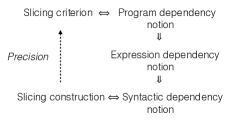
Figure 13: Schema of dependency-based slicing notions.

In Figure 13 we show these relations. In particular, starting from the criterion, we can define an equivalent notion of dependency which allows us to identify which variables should be kept in a slice, affecting the whole program semantics (program dependency notion).

Definition 5.2 ((Semantic) Program dependency)

Let be a slicing criterion, and $P$ be a program. The program depends on $x$, denoted $x{\rightsquigarrow}_{\mbox{\tiny\sc$\crit$}}P$ iff

$$\exists\mu_{1},\mu_{2}\in{\mathcal{I}}.\>\forall y\neq x.\>\mu_{1}(y)=\mu_{2}(y)\ \wedge\ \mathit{Proj}_{({\mathcal{X}},{\mathcal{O}},{\mathcal{L}})}(\tau_{P}^{\mu_{1}})\neq\mathit{Proj}_{({\mathcal{X}},{\mathcal{O}},{\mathcal{L}})}(\tau_{P}^{\mu_{2}})$$

This means that the variable $x$ affects the observable semantics of $P$.

Unfortunately, this characterization is not effective due to undecidability of the program semantics. In particular, the amount of traces to compare could be infinite, and also the traces themselves could be infinite. Hence, we consider a stronger notion of dependency that looks for local semantic dependencies, identifying all the variables affecting at least one expression used in the program (expression dependency notion), and this is precisely the semantic generalization of the syntactic dependency notion used, for instance, in PDG-based algorithm for slicing. In other words we characterize when a variable affects the semantics of an expression in $P$.

Our idea is to make semantic the standard notion of syntactic dependency, by substituting the notion of uses with the notion of depends on [Giacobazzi et al. (2012)]. In order to obtain this characterization, we have to find which variables might affect the evaluation of the expression $e$ in the assignment z:=e or in a control statement guarded by $e$, i.e., which variables belong to the set $\textsc{rel}\left(e\right)$ of the variables relevant to the evaluation of $e$. As already pointed out, standard syntactic dependency calculi compute $\textsc{rel}\left(e\right)$ as $\textsc{vars}\left(e\right)$.

Definition 5.3 ((Semantic) Expression dependency)

Let be a slicing criterion. Let $x\in\mathbb{X}$, ${\mathcal{Y}}\subseteq\mathbb{X}$.

$$\begin{array}[]{rcl}x{\rightsquigarrow}_{\mbox{\tiny\sc$\crit$}}e&\Leftrightarrow&\exists\sigma_{1},\sigma_{2}\in\Sigma.\ \forall y\neq x.\>\sigma_{1}(y)=\sigma_{2}(y)\wedge\ \mbox{\raisebox{0.0pt}[4.30554pt][4.30554pt]{$\left\llbracket e\right\rrbracket\left(\sigma_{1}\right)$}}\neq\mbox{\raisebox{0.0pt}[4.30554pt][4.30554pt]{$\left\llbracket e\right\rrbracket\left(\sigma_{2}\right)$}}\\ {\mathcal{Y}}{\rightsquigarrow}_{\mbox{\tiny\sc$\crit$}}e&\Leftrightarrow&\exists y\in{\mathcal{Y}}.\ y{\rightsquigarrow}_{\mbox{\tiny\sc$\crit$}}e\\ &\Leftrightarrow&\exists\sigma_{1},\sigma_{2}\in\Sigma.\ \forall w\notin{\mathcal{Y}}.\>\sigma_{1}(w)=\sigma_{2}(w)\wedge\ \mbox{\raisebox{0.0pt}[4.30554pt][4.30554pt]{$\left\llbracket e\right\rrbracket\left(\sigma_{1}\right)$}}\neq\mbox{\raisebox{0.0pt}[4.30554pt][4.30554pt]{$\left\llbracket e\right\rrbracket\left(\sigma_{2}\right)$}}\\ \end{array}$$

The formulation of $x{\rightsquigarrow}_{\mbox{\tiny\sc$\crit$}}e$ can be rewritten as

$$\exists\sigma\in\Sigma,v_{1},v_{2}\in\mathbb{V}.\>\mbox{\raisebox{0.0pt}[4.30554pt][4.30554pt]{$\left\llbracket e\right\rrbracket\left(\sigma\left[x\leftarrow v_{1}\right]\right)$}}\neq\mbox{\raisebox{0.0pt}[4.30554pt][4.30554pt]{$\left\llbracket e\right\rrbracket\left(\sigma\left[x\leftarrow v_{2}\right]\right)$}}$$

Proposition 5.4.

Let be a slicing criterion. If $x{\rightsquigarrow}_{\mbox{\tiny\sc$\crit$}}P$ then there exists $e$ in $P$ such that $x{\rightsquigarrow}_{\mbox{\tiny\sc$\crit$}}e$.

Proof 5.5.

Let us reason by contradiction. If for each $e$ in $P$ we have $x{\not\rightsquigarrow}_{\mbox{\tiny\sc$\crit{}_{\mathcal{A}}$}}e$, then all the expressions in $P$ do not depend on $x$ and therefore, independently from $x$, $P$ provides precisely the same results.

By using this notion of dependency, we can characterize the subset $\textsc{rel}\left(e\right)\subseteq\textsc{vars}\left(e\right)$ containing exactly those variables which are semantically relevant for the evaluation of $e$. This way, we obtain a notion of dependency which allows us to derive more precise slices, i.e., to remove statements that a merely syntactic analysis would leave.

Example 5.6.

Consider the program $P$:

⬇

1 x:=$e_{x}$;

2 y:=$e_{y}$;

3 w:=$e_{w}$;

4 z:=w+y+2(x²)-w;

where $e_{x}$, $e_{y}$ and $e_{w}$ are expressions. We want to compute the static slice $Q$ of $P$ affecting the final value of z (i.e., the slicing criterion is interested in the final value of z). If we consider the traditional notion of slicing, then it is clear that we can erase line 3 without changing the final result for z. However, in the usual syntactic approach, we would have a dependency between z and w, since w is used where z is defined. Consequently, the slice obtained by applying this form of dependency would leave the program unchanged. On the other hand, if the semantic dependency is considered, then the evaluation of ${{{{\mbox{$\mbox{\leavevmode\lstinline{{\lst@@@set@language\lst@@@set@numbers\lst@@@set@frame\lst@@@set@rulecolor\lst@@@set@frame\lst@@@set@numbers\lst@@@set@language\small\rm{\@listingGroup{ltx_lst_identifier}{w}}}}}}$}+\mbox{$\mbox{\leavevmode\lstinline{{\lst@@@set@language\lst@@@set@numbers\lst@@@set@frame\lst@@@set@rulecolor\lst@@@set@frame\lst@@@set@numbers\lst@@@set@language\small\rm{\@listingGroup{ltx_lst_identifier}{y}}}}}}$}+2(\mbox{$\mbox{\leavevmode\lstinline{{\lst@@@set@language\lst@@@set@numbers\lst@@@set@frame\lst@@@set@rulecolor\lst@@@set@frame\lst@@@set@numbers\lst@@@set@language\small\rm{\@listingGroup{ltx_lst_identifier}{x}}}}}}$}^{2})-\mbox{$\mbox{\leavevmode\lstinline{{\lst@@@set@language\lst@@@set@numbers\lst@@@set@frame\lst@@@set@rulecolor\lst@@@set@frame\lst@@@set@numbers\lst@@@set@language\small\rm{\@listingGroup{ltx_lst_identifier}{w}}}}}}$}$ does not depend on the possible variations of w, which implies that we are able to erase line 3 from the slice.

Next we show how the PDG-based approach to slicing can be modified in order to cope with semantic slicing. The PDG approach is based on the computation of the set of variables used in a expression $e$. In the following, we wonder if this set can be rewritten by considering a semantic form of dependency.

Hence, let us define the new notion of semantic PDG, where all the flow dependencies are semantic, i.e., we substitute the flow edges defined above with semantic flow dependency edges $u\longrightarrow_{sf}v$ which are such that (1) $u$ is a node that defines the variable $x$ (usually an assignment), (2) $v$ is a node containing an expression $e$ such that $x{\rightsquigarrow}_{\mbox{\tiny\sc$\crit$}}e$ (where is the criterion with respect with we are computing the slice), and (3) control can reach $v$ from $u$ via an execution path along which there is no intervening re-definition of $x$. A (semantic) flow path is a sequence of (semantic) flow edges.

Proposition 5.7.

Let $P$ be a program and be a slicing criterion. Let ${\mathcal{G}}_{P}$ the PDG with flow dependency edges $\longrightarrow_{f}$, and ${\mathcal{G}}_{P}^{s}$ be the semantic PDG where the flow dependency edge are semantic $\longrightarrow_{sf}$. If $u\longrightarrow_{sf}v$ then $u\longrightarrow_{f}v$.

Proof 5.8.

Trivially, since if $x{\rightsquigarrow}_{\mbox{\tiny\sc$\crit$}}e$, then $e$ must use the variable $x$.

In principle, a (backward) slice is composed by all the statements (i.e., nodes) such that there exists a path from the corresponding node to the relevant (according to the slicing criterion) use of a variable of interest (in the criterion) [Reps and Yang (1989)]. In other words, we follow backward the (semantic) flow edges from the nodes identified by the criterion, and we keep all the nodes/statements we reach. Hence, the criterion, and therefore the dependency notion, defines the edges that we can follow for computing the slice.

By using the semantic flow dependency edges, we can draw a new semantic PDG containing less flow edges, i.e., only those corresponding to semantic dependencies. At this point, the type of slicing (either static, dynamic or conditional) characterized by the criterion decides which nodes can be kept in the PDG.

Theorem 5.9.

Let ${\mathcal{C}}=\langle{\mathcal{I}},{\mathcal{X}},{\mathcal{O}},\psi\rangle$ be a slicing criterion. Let $P$ be a program and ${\mathcal{G}}^{s}_{P}$ its semantic PDG, i.e., a PDG whose flow edges are $\longrightarrow_{sf}$. Let $Q$ the subprogram of $P$ containing all the statements corresponding to nodes such that there exists a semantic flow path in ${\mathcal{G}}^{s}_{P}$ from them to a node in ${\mathcal{N}}_{{\mathcal{O}}}\mbox{\raisebox{0.0pt}[4.30554pt][4.30554pt]{$\stackrel{{\scriptstyle\mbox{\tiny def}}}{{\;=\;}}$}}\left\{~{}n~{}\left|\begin{array}[]{l}\exists\langle n,K\rangle\in{\mathcal{O}}\end{array}\right.\right\}$. Then $Q$ is a slice w.r.t. the criterion ${\mathcal{C}}$.

Proof 5.10.

Note that, the PDG construction is syntactic, and therefore independent from the input set ${\mathcal{I}}$, hence any slice computed by using the PDG holds for any possible input memory in $\mathbb{M}$. Moreover, since we simply collects the statements potentially affecting the program observation, we cannot decide which iteration to observe, for this reason each program point is taken in the slice independently from the iteration to observe, for this reason the obtained slice will provide the same result for any possible iteration, i.e., the set of interesting points to observe are ${\mathcal{N}}_{\mathcal{O}}\times\{\mathbb{N}\}=\left\{~{}\langle n,\mathbb{N}\rangle~{}\left|\begin{array}[]{l}n\in{\mathcal{N}}_{{\mathcal{O}}}\end{array}\right.\right\}$. Finally, by construction we cannot have statements executed in the slice which are not executed in the original programs. Hence, the criterion enforced by the PDG slice construction is (direct consequence of the Slicing theorem in [Reps and Yang (1989)]), which for each ${\mathcal{I}}\subseteq\mathbb{M}$ and $\{K_{n}\}_{n\in{\mathcal{N}}_{\mathcal{O}}}\subseteq\wp(\mathbb{N})$ is a slice also w.r.t. the criterion $({\mathcal{I}},{\mathcal{X}},\{\langle n,K_{n}\rangle~{}|~{}n\in{\mathcal{N}}_{\mathcal{O}}\},\psi)$, by [Binkley et al. (2006a)] (Equation 2 in the Appendix). Hence, we have that the results is a slice w.r.t.  [Binkley et al. (2006a)].

We have pointed out so far the difference between syntactic and semantic dependencies: it can be the case that a variable syntactically appears in an expression without affecting its value. Actually, one could argue that the case is not very likely to happen: the possibility to find an assignment like x:=y-y in code written by a professional software engineer is remote to the very least. However, when it comes to abstract dependencies, the picture is quite different, and we could even say that, in the present work, (concrete) semantic dependencies have been mainly introduced to prepare the discussion about their abstract counterpart. Indeed, it is much more likely that some variables are not semantically relevant to an expression if the value of interest is an abstract one, e.g., the parity or the sign of a numeric expression, or the nullity of a pointer. This justifies the definition of a semantic notion of dependency at the abstract level.

6 Abstract Dependencies

This section discusses the problem of defining and computing abstract dependencies allowing us to capture the dependency relation between variables w.r.t. a given abstract criterion. In the previous section, we formalized this relation in the concrete semantic case; the following example takes it to the abstract level.

Example 6.1.

Consider the expression $e=$ 2x²+y: although both variables are semantically relevant to the result, only y can affect its parity, since 2x² will always be even. On the other hand, note that both variables are relevant to the sign of $e$, in spite of the positivity of x². In fact, given a negative value for y, a change in the value of x can alter the sign of the entire expression.

First of all, it is worth noting that the notion of semantic program dependency can be easily extended to abstract criteria, simply by changing the projection considered. In this case we will write that $x{\rightsquigarrow}_{\mbox{\tiny\sc$\crit{}_{\mathcal{A}}$}}P$, meaning that $x$ has effect on the abstract projection of $P$ determined by . Also in the abstract case we inherit the undecidability of the concrete semantics of $P$; hence, again, we have to approximate the semantic program dependency with a local notion of abstract semantic expression dependency. Unfortunately, when dealing with abstract criteria , some aspects become more complicated.

6.1 Abstract slicing and dependencies

In the previous section, we defined the concrete semantic dependency by identifying those variables that do not interfere with the final observation of each expression. Analogously, in order to define a general notion of abstract semantic dependency, we need to consider the abstract interference between a property of a variable and a property of an expression.

The definition below follows the same philosophy as narrow abstract non-interference [Giacobazzi and Mastroeni (2004a), Mastroeni (2013)], where abstractions for observing input and output are considered, but these abstractions are observations of the concrete executions.

Definition 6.2 ((Abstract) Semantic expression dependency, Ndep)

Consider the abstractions $\rho\in\mbox{\sl uco}(\wp(\mathbb{V}))$ and $\overline{\eta}\in\mbox{\sl uco}(\wp(\mathbb{V}))^{n}$, where $n$ is the number of variables, i.e., $\overline{\eta}$ is a tuple of properties such that $\eta_{y}$ is the property on the variable $y$.

$$\begin{array}[]{rcl}\mbox{\raisebox{0.0pt}[4.30554pt][4.30554pt]{$x\mathrel{\vbox{\offinterlineskip\halign{\hfil#\hfil\cr{\tiny$\overline{\eta},\rho$}\cr\kern-0.43057pt\cr$\rightsquigarrow\!\rightsquigarrow\!\rightsquigarrow$\cr}}}e$}}&\Leftrightarrow&\exists\sigma_{1},\sigma_{2}\in\Sigma\>.\ \left(\forall y\neq x.\>\eta_{y}(\sigma_{1}(y))=\eta_{y}(\sigma_{2}(y))\ \wedge\ \rho(\mbox{\raisebox{0.0pt}[4.30554pt][4.30554pt]{$\left\llbracket e\right\rrbracket\left(\sigma_{1}\right)$}})\neq\rho(\mbox{\raisebox{0.0pt}[4.30554pt][4.30554pt]{$\left\llbracket e\right\rrbracket\left(\sigma_{2}\right)$}})\right)\\ \end{array}$$

This notion is a generalization of Definition 5.3 where we abstract the observation of the result ($\rho$) and the information that we fix about all the variables different from x ($\overline{\eta}$). Still, this notion characterizes whether the variation of the value of x affects the abstract evaluation in $\rho$ of $e$.

As an important result, we have $\mbox{\raisebox{0.0pt}[4.30554pt][4.30554pt]{$x\mathrel{\vbox{\offinterlineskip\halign{\hfil#\hfil\cr{\tiny$\overline{\eta},\rho^{1}$}\cr\kern-0.43057pt\cr$\rightsquigarrow\!\rightsquigarrow\!\rightsquigarrow$\cr}}}e$}}\Leftrightarrow\mbox{\raisebox{0.0pt}[4.30554pt][4.30554pt]{$x\mathrel{\vbox{\offinterlineskip\halign{\hfil#\hfil\cr{\tiny$\overline{\eta},\rho^{2}$}\cr\kern-0.43057pt\cr$\rightsquigarrow\!\rightsquigarrow\!\rightsquigarrow$\cr}}}e$}}$ whenever $\rho^{1}$ and $\rho^{2}$ induce the same partitions (either on values, or tuples of values). This happens because, in Definition 6.2, both abstractions are only applied to singletons. In the following, only partitioning domains will be considered since it is straightforward to note that $x\mathrel{\vbox{\offinterlineskip\halign{\hfil#\hfil\cr{\tiny$\overline{\eta},\rho$}\cr\kern-0.43057pt\cr$\rightsquigarrow\!\rightsquigarrow\!\rightsquigarrow$\cr}}}e$ is affected only by $\Pi(\rho)$, rather than by $\rho$ itself.

When dealing with abstractions, and therefore with abstract computations, some more considerations have to be taken into account. Consider the program in Example 5.6, and consider the $\rho_{\textsc{par}}$ property (Section 2.2) for all variables on both input and output . If we compute the set of variables on which the parity of $e=$ w+y+2(x²)-w depends on, then we can observe that $e$ is still independent from w, but is also independent from any possible variation of x. At a first sight, the parity of w+y+2(x²)-w is independent from x just because 2(x²) is constantly even. However, it is not only a matter of constancy: a deeper analysis would note that we can look simply at the abstract value of x only because the operation involved (the sum) in the evaluation is complete (Section 2.2), i.e., precise, w.r.t. the abstract domain considered ($\rho_{\textsc{par}}$). In particular, when we deal with abstract domains which are complete for the considered operations, then it is enough to look at the abstract value of variables in order to compute dependencies. Indeed, consider the $\rho_{\textsc{sign}}$ domain (Section 2.2). In this case, even if the sign of 2(x²) is constantly positive, the final sign of z might be affected by a concrete variation of x (e.g., consider ${\mbox{$\mbox{\leavevmode\lstinline{{\lst@@@set@language\lst@@@set@numbers\lst@@@set@frame\lst@@@set@rulecolor\lst@@@set@frame\lst@@@set@numbers\lst@@@set@language\small\rm{\@listingGroup{ltx_lst_identifier}{y}}}}}}$}=-4$ and two executions in which x is, respectively, 1 and 5). Therefore, x has to be considered relevant, although the sign of 2(x²) (the only sub-expression containing x) is constant. This can be also derived by considering the logic of independencies from [Amtoft and Banerjee (2007)] since, by varying the value of x, we can change the sign of $e$.

Unfortunately, the notion of abstract dependencies given in Definition 6.2 is not suitable for weakening the PDG approach, as we have done in the concrete semantic case. Let us explain the problem in the following example.

Example 6.3.

Consider the program $P=$C; x:=y>0?0:1;, where C is come code fragment and the expression b?e1:e2 evaluates to e1 if b is true, and to e2 otherwise.

Suppose the criterion requires the observation of the parity of $x$ at this program point, i.e., ${\mathcal{A}}=\langle x:\rho_{\textsc{par}}\rangle$. Then it is straightforward to observe that the expression depends on $y$, but we would like to be more specific (being in the context of abstract slicing), and we can observe that it is the sign of $y$ that affects the parity of the expression, and therefore of $x$. At this point, in the code C we should look for the variables affecting not simply $y$ (as expected in standard slicing approaches), but more specifically the sign of $y$, a requirement not considered in the abstract criterion.

This example shows that, if we aim at computing abstract dependencies without losing too much information, we would need an algorithm able to keep trace backwards, not only of the different variables that become of interest (affecting the desired criterion), but also of the different properties to observe on variables affecting the desired property of the criterion. This means that, while for the concrete semantic program dependency we can provide a definition depending only on the criterion, this is not possible in a more abstract context, where each flow edge should be defined depending on abstract properties potentially different from those in the abstract criterion, and which should be characterized dynamically backward starting from the criterion. Unfortunately, this is not possible in Definition 6.2, where we always look for the variation of the value and not of an abstract property of x, hence if we would use this notion for substituting the semantic dependency in PDGs we would not have so much advantage.

These observations make clear that, if we aim at constructively characterize abstract slicing by means of the abstract dependency notion provided in Definition 6.2, we need to build from scratch a systematic approach for characterizing abstract slicing. Towards this direction, the first step we propose is a computable approximation of the abstract dependencies of Definition 6.2.

6.2 A constructive approach to Abstract Dependencies

By means of the (uco-dependent) definition of operations on abstract values, it is possible to automatically obtain (an over-approximation of) the set of relevant variables. The starting point is the brute-force approach which uses the abstract version of concrete operations, and explicitly goes into the quantifiers involved in Definition 6.2.

Example 6.4.

Consider the program in Example 5.6 and let $\eta_{y}=\rho_{\textsc{par}}$. In order to decide whether ${{}\mbox{$\mbox{\leavevmode\lstinline{{\lst@@@set@language\lst@@@set@numbers\lst@@@set@frame\lst@@@set@rulecolor\lst@@@set@frame\lst@@@set@numbers\lst@@@set@language\small\rm{\@listingGroup{ltx_lst_identifier}{x}}}}}}$}\mathrel{\vbox{\offinterlineskip\halign{\hfil#\hfil\cr{\tiny$\overline{\eta},\rho$}\cr\kern-0.43057pt\cr$\rightsquigarrow\!\rightsquigarrow\!\rightsquigarrow$\cr}}}e$ holds, the brute-force approach considers the abstract evaluation of $e$ in all contexts where all variables different from x does not change, up to $\overline{\eta}$, while x may change. In this example, this boils down to consider pairs of memories where y has the same parity (with no information about sign), and we take memories where x changes value, and see whether the final values of $e$ agree on the expression observation $\rho$. Suppose ${\rho_{\textsc{par}}(\mbox{\leavevmode\lstinline{{\lst@@@set@language\lst@@@set@numbers\lst@@@set@frame\lst@@@set@rulecolor\lst@@@set@frame\lst@@@set@numbers\lst@@@set@language\small\rm{\@listingGroup{ltx_lst_identifier}{y}}}}}})=\left[\mathbf{even}\right]$ (meaning that it is even but the sign is unknown) and suppose $\rho=\rho_{\textsc{sign}}$, then we should have to compute the abstract value of $e$ for each possible value for x. It is clear that we can easily find $\sigma_{1}$ and $\sigma_{2}$ such that

$${{{{2*\sigma_{1}(\mbox{\leavevmode\lstinline{{\lst@@@set@language\lst@@@set@numbers\lst@@@set@frame\lst@@@set@rulecolor\lst@@@set@frame\lst@@@set@numbers\lst@@@set@language\small\rm{\@listingGroup{ltx_lst_identifier}{x}}}}}})^{2}+\sigma_{1}(\mbox{\leavevmode\lstinline{{\lst@@@set@language\lst@@@set@numbers\lst@@@set@frame\lst@@@set@rulecolor\lst@@@set@frame\lst@@@set@numbers\lst@@@set@language\small\rm{\@listingGroup{ltx_lst_identifier}{y}}}}}})=\left[\mathbf{neg}\right],\qquad 2*\sigma_{2}(\mbox{\leavevmode\lstinline{{\lst@@@set@language\lst@@@set@numbers\lst@@@set@frame\lst@@@set@rulecolor\lst@@@set@frame\lst@@@set@numbers\lst@@@set@language\small\rm{\@listingGroup{ltx_lst_identifier}{x}}}}}})^{2}+\sigma_{2}(\mbox{\leavevmode\lstinline{{\lst@@@set@language\lst@@@set@numbers\lst@@@set@frame\lst@@@set@rulecolor\lst@@@set@frame\lst@@@set@numbers\lst@@@set@language\small\rm{\@listingGroup{ltx_lst_identifier}{y}}}}}})=\left[\mathbf{pos}\right]$$

even if ${{\rho_{\textsc{par}}(\sigma_{1}(\mbox{\leavevmode\lstinline{{\lst@@@set@language\lst@@@set@numbers\lst@@@set@frame\lst@@@set@rulecolor\lst@@@set@frame\lst@@@set@numbers\lst@@@set@language\small\rm{\@listingGroup{ltx_lst_identifier}{y}}}}}}))=\rho_{\textsc{par}}(\sigma_{2}(\mbox{\leavevmode\lstinline{{\lst@@@set@language\lst@@@set@numbers\lst@@@set@frame\lst@@@set@rulecolor\lst@@@set@frame\lst@@@set@numbers\lst@@@set@language\small\rm{\@listingGroup{ltx_lst_identifier}{y}}}}}}))$ (for instance ${{\sigma_{1}(\mbox{\leavevmode\lstinline{{\lst@@@set@language\lst@@@set@numbers\lst@@@set@frame\lst@@@set@rulecolor\lst@@@set@frame\lst@@@set@numbers\lst@@@set@language\small\rm{\@listingGroup{ltx_lst_identifier}{y}}}}}})=\sigma_{2}(\mbox{\leavevmode\lstinline{{\lst@@@set@language\lst@@@set@numbers\lst@@@set@frame\lst@@@set@rulecolor\lst@@@set@frame\lst@@@set@numbers\lst@@@set@language\small\rm{\@listingGroup{ltx_lst_identifier}{y}}}}}})=-4$ while ${\sigma_{1}(\mbox{\leavevmode\lstinline{{\lst@@@set@language\lst@@@set@numbers\lst@@@set@frame\lst@@@set@rulecolor\lst@@@set@frame\lst@@@set@numbers\lst@@@set@language\small\rm{\@listingGroup{ltx_lst_identifier}{x}}}}}})=1$ and ${\sigma_{2}(\mbox{\leavevmode\lstinline{{\lst@@@set@language\lst@@@set@numbers\lst@@@set@frame\lst@@@set@rulecolor\lst@@@set@frame\lst@@@set@numbers\lst@@@set@language\small\rm{\@listingGroup{ltx_lst_identifier}{x}}}}}})=5$). It is clear that the sign of $e$ may depend on the value of x since to “fix” the abstract property of the other variables is not enough to “fix” the final value of $e$ w.r.t. $\rho$. On the other hand, the parity of $e$ does not depend on x, in particular if we fix the property $\rho_{\textsc{par}}$ of y, for instance to $\left[\mathbf{even}\right]$ (but it holds also for the other abstract values) then

$$2*\left[\mathbf{negodd}\right]^{2}+\left[\mathbf{even}\right]=\left[\mathbf{poseven}\right],\qquad 2*\left[\mathbf{poseven}\right]^{2}+\left[\mathbf{even}\right]=\left[\mathbf{even}\right]\qquad\ldots$$

Namely, if we fix all the (abstract values of the) variables but x, then the parity of the result does not change, hence the variation of x does not affect the parity of the expression $e$.

In the following, we introduce an algorithm able to improve the computational complexity of the brute-force approach, especially on bigger ucos, and when (1) several variables are involved in expressions, and (2) a significant part of them is irrelevant.

6.2.1 Checking Ndep

In the following, we discuss how we can constructively compute narrow dependencies. Unfortunately, in static analysis, the concrete semantics cannot be used directly as it appears in Definition 6.2, hence we need to approximate this abstract notion. The following definition introduces a stronger notion of dependency based on a sound abstract semantics $\left\llbracket\cdot\right\rrbracket^{\rho}$ (Section 2.4), which approximates narrow dependencies.

Definition 6.5 (Atom-dep)

An expression $e$ atom-depends on $x$ (written $x\mathrel{\vbox{\offinterlineskip\halign{\hfil#\hfil\cr{\tiny$\overline{\eta},\rho$}\cr\kern-0.43057pt\cr$\rightsquigarrow\!\rightsquigarrow\!\rightsquigarrow$\cr}}}_{\mbox{\tiny\sc at}}e$) with respect to $\rho\in\mbox{\sl uco}(\wp(\mathbb{V}))$ and $\overline{\eta}\in\mbox{\sl uco}(\wp(\mathbb{V}))^{n}$ ($n$ number of variables) if and only if there exist $\sigma_{1},\sigma_{2}\in\Sigma$ such that

$$\forall y\neq x.\eta_{y}(\sigma_{1}(y))=\eta_{y}(\sigma_{2}(y))\ \quad\wedge\ \quad\neg\textsc{Atom}_{\rho}\left(\mbox{\raisebox{0.0pt}[4.30554pt][4.30554pt]{$\left\llbracket e\right\rrbracket^{\rho}\left(\{\sigma_{1},\sigma_{2}\}\right)$}}\right)$$

Being domains partitioning, the non-atomicity requirement $\neg\textsc{Atom}_{\rho}\left(\cdot\right)$ amounts to say that all $\rho$-abstract evaluations of $e$, starting from different values for $x$, may not be abstracted in the same abstract value (this is the crucial issue in Ndep), i.e., $\sigma_{1}$ and $\sigma_{2}$ may lead to different abstract values for $e$. Next results shows that Atom-dep is an approximation of Ndep, since Ndep implies Atom-dep, meaning that Atom-dep may only add false dependencies, but cannot lose abstract dependencies characterized by Ndep.

Proposition 6.6.

Consider the abstractions $\rho\in\mbox{\sl uco}(\wp(\mathbb{V}))$ and $\overline{\eta}\in\mbox{\sl uco}(\wp(\mathbb{V}))^{n}$, where $n$ is the number of variables, i.e., $\overline{\eta}$ is a tuples of properties. For every $e$ and $x$, $x\mathrel{\vbox{\offinterlineskip\halign{\hfil#\hfil\cr{\tiny$\overline{\eta},\rho$}\cr\kern-0.43057pt\cr$\rightsquigarrow\!\rightsquigarrow\!\rightsquigarrow$\cr}}}e$ implies $x\mathrel{\vbox{\offinterlineskip\halign{\hfil#\hfil\cr{\tiny$\overline{\eta},\rho$}\cr\kern-0.43057pt\cr$\rightsquigarrow\!\rightsquigarrow\!\rightsquigarrow$\cr}}}_{\mbox{\tiny\sc at}}e$.

Proof 6.7.

Suppose $x\mathrel{\vbox{\offinterlineskip\halign{\hfil#\hfil\cr{\tiny$\overline{\eta},\rho$}\cr\kern-0.43057pt\cr$\rightsquigarrow\!\rightsquigarrow\!\rightsquigarrow$\cr}}}e$, i.e., $\exists\sigma_{1},\sigma_{2}\in\Sigma\>.\ (1)\>\forall y\neq x.\>\eta_{y}\left(\sigma_{1}\right)=_{y}\eta_{y}\left(\sigma_{2}\right)\ \wedge\ (2)\>\rho(\mbox{\raisebox{0.0pt}[4.30554pt][4.30554pt]{$\left\llbracket e\right\rrbracket\left(\sigma_{1}\right)$}})\neq\rho(\mbox{\raisebox{0.0pt}[4.30554pt][4.30554pt]{$\left\llbracket e\right\rrbracket\left(\sigma_{2}\right)$}})$, then we have to prove $x\mathrel{\vbox{\offinterlineskip\halign{\hfil#\hfil\cr{\tiny$\overline{\eta},\rho$}\cr\kern-0.43057pt\cr$\rightsquigarrow\!\rightsquigarrow\!\rightsquigarrow$\cr}}}_{\mbox{\tiny\sc at}}e$, i.e., there exist $\sigma_{1},\sigma_{2}\in\Sigma$ such that $(3)\>\forall y\neq x.\eta_{y}\left(\sigma_{1}\right)=_{y}\eta_{y}\left(\sigma_{2}\right)$ and $(4)\>\neg\textsc{Atom}_{\rho}\left(\mbox{\raisebox{0.0pt}[4.30554pt][4.30554pt]{$\left\llbracket e\right\rrbracket^{\rho}\left(\{\sigma_{1},\sigma_{2}\}\right)$}}\right)$. Since conditions $(1)$ and $(3)$ are the same, we have to prove that $\exists\sigma_{1},\sigma_{2}\in\Sigma.\>(2)\Rightarrow(4)$.

Consider $\sigma_{1},\sigma_{2}\in\Sigma$ satisfying $(1)$ and such that $\rho(\mbox{\raisebox{0.0pt}[4.30554pt][4.30554pt]{$\left\llbracket e\right\rrbracket\left(\sigma_{1}\right)$}})\neq\rho(\mbox{\raisebox{0.0pt}[4.30554pt][4.30554pt]{$\left\llbracket e\right\rrbracket\left(\sigma_{2}\right)$}})$, then $\rho(\mbox{\raisebox{0.0pt}[4.30554pt][4.30554pt]{$\left\llbracket e\right\rrbracket\left(\sigma_{1}\right)$}}),\rho(\mbox{\raisebox{0.0pt}[4.30554pt][4.30554pt]{$\left\llbracket e\right\rrbracket\left(\sigma_{2}\right)$}})\in\rho(\mbox{\raisebox{0.0pt}[4.30554pt][4.30554pt]{$\left\llbracket e\right\rrbracket\left(\{\sigma_{1},\sigma_{2}\}\right)$}})\subseteq\rho(\mbox{\raisebox{0.0pt}[4.30554pt][4.30554pt]{$\left\llbracket e\right\rrbracket\left(\rho(\{\sigma_{1},\sigma_{2}\})\right)$}})=\mbox{\raisebox{0.0pt}[4.30554pt][4.30554pt]{$\left\llbracket e\right\rrbracket^{\rho}\left(\{\sigma_{1},\sigma_{2}\}\right)$}}$. At this point, since $\left\llbracket e\right\rrbracket^{\rho}\left(\{\sigma_{1},\sigma_{2}\}\right)$ contains two different values of $\rho$, then, by definition, it cannot be an atom of $\rho$.

Starting from this new approximate notion, our idea is to provide an algorithm over-approximating the set of variables relevant for a given expression $e$ when $\forall y\neq x.\eta_{y}=\rho$, namely the abstraction observed in output is the same that we fix on the input variables. The idea is to start from an empty set of not relevant variables $X$ for an expression $e$, and incrementally increase this set adding all those variables that surely are not relevant for the expression (obtaining an under-approximation of abstract dependencies). Finally, the complement of such set is returned, which is an over-approximation of relevant variables.

In order to check the dependency relation, we aim at checking whether a change of the values of a variables makes a difference in the evaluation of the expression. Dependencies are computed according to Atom-dep, in order to approximate Ndep. In a brute-force approach, Atom-dep would be verified by checking for each ${\sigma^{\rho}}$ associating atomic values to variables we have that $\textsc{Atom}_{\rho}\left(\mbox{\raisebox{0.0pt}[4.30554pt][4.30554pt]{$\left\llbracket e\right\rrbracket^{\rho}\left({\sigma^{\rho}}\right)$}}\right)$ is always the same atom.

Example 6.8.

Let $e$ be an expression involving variables $x$, $y$ and $z$, and $\rho=\rho_{\textsc{parSign}}$. In principle, in order to compute the set of $\rho$-dependencies on $e$, we must compute $\left\llbracket e\right\rrbracket^{\rho}$ on every possible atomic value of x, y and z, i.e., $\left\llbracket e\right\rrbracket^{\rho}$ must be computed $5^{3}=125$ times. y is not relevant to $e$ if, for any abstract values $\mbox{{\sc{v}}}_{x},\mbox{{\sc{v}}}_{z}\in\textsc{Atoms}\left(\rho\right)$, there exists an atomic abstract value $\mbox{{\sc{u}}}\in\textsc{Atoms}\left(\rho\right)$ such that $\forall\mbox{{\sc{v}}}\in\textsc{Atoms}\left(\rho\right).\ \mbox{{\sc{u}}}=\mbox{\raisebox{0.0pt}[4.30554pt][4.30554pt]{$\left\llbracket e\right\rrbracket^{\rho}\left(\{x\!\leftarrow\!\mbox{{\sc{v}}}_{x},y\!\leftarrow\!\mbox{{\sc{v}}},z\!\leftarrow\!\mbox{{\sc{v}}}_{z}\}\right)$}}$. This amounts to say that changing the value of y does not affect $e$, since we require the same output atomic evaluation for each possible abstract value for y. Indeed, if the result is not atomic, it means that we have at least two different abstract results for different values of y. Analogously, for different (abstract) values for y we have different atomic results, then again it means that there exists a variation of y affecting the abstract evaluation of $e$.

However, it is possible to be smarter:

• Excluding states: consider dependencies of $e$ in Example 6.8, computed at program point $n$. Suppose $\left\llbracket\cdot\right\rrbracket^{\rho}$ (used as a tool to infer invariant properties, as discussed in Section 2.4) is able to infer, at point $n$, that the abstract state ${\sigma^{\rho}_{n}}$ is such that ${{\sigma^{\rho}_{n}}(\mbox{\leavevmode\lstinline{{\lst@@@set@language\lst@@@set@numbers\lst@@@set@frame\lst@@@set@rulecolor\lst@@@set@frame\lst@@@set@numbers\lst@@@set@language\small\rm{\@listingGroup{ltx_lst_identifier}{y}}}}}})=\left[\mathbf{posodd}\right]$ correctly approximates the value of variables at $n$. Then, we only need to consider states of the form $\{x\!\leftarrow\!\mbox{{\sc{v}}}_{x},y\!\leftarrow\!\left[\mathbf{posodd}\right],z\!\leftarrow\!\mbox{{\sc{v}}}_{z}\}$ as inputs for $\left\llbracket e\right\rrbracket^{\rho}$ (now considered as the abstract computation of expressions, according to Definition 6.5) at $n$.

• Computing on non-atomic states: let $E=\{\left[\mathbf{poseven}\right],\left[\mathbf{zero}\right],\left[\mathbf{negeven}\right]\}$ and $O=\{\left[\mathbf{posodd}\right],\left[\mathbf{negodd}\right]\}$. In this case,

  $$\forall\mbox{{\sc{v}}}^{\prime}\in E,\mbox{{\sc{v}}}^{\prime\prime}\in O.\ \mbox{\raisebox{0.0pt}[4.30554pt][4.30554pt]{$\left\llbracket e\right\rrbracket^{\rho}\left(\{x\!\leftarrow\!\mbox{{\sc{v}}}_{x},y\!\leftarrow\!\mbox{{\sc{v}}}^{\prime},z\!\leftarrow\!\mbox{{\sc{v}}}\}\right)$}}\leq\mbox{{\sc{u}}}$$

  is implied by the more general result

  $$\mbox{\raisebox{0.0pt}[4.30554pt][4.30554pt]{$\left\llbracket e\right\rrbracket^{\rho}\left(\{x\!\leftarrow\!\mbox{{\sc{v}}}_{x},y\!\leftarrow\!\left[\mathbf{even}\right],z\!\leftarrow\!\left[\mathbf{odd}\right]\}\right)$}}\leq\mbox{{\sc{u}}}$$

  since $E$ and $O$ are partitions, respectively, of $\left[\mathbf{even}\right]$ and $\left[\mathbf{odd}\right]$, and $\left\llbracket e\right\rrbracket^{\rho}$ is monotone: ${\sigma^{\rho}_{1}}\leq{\sigma^{\rho}_{2}}$ implies $\Rightarrow\mbox{\raisebox{0.0pt}[4.30554pt][4.30554pt]{$\left\llbracket e\right\rrbracket^{\rho}\left({\sigma^{\rho}_{1}}\right)$}}\leq\mbox{\raisebox{0.0pt}[4.30554pt][4.30554pt]{$\left\llbracket e\right\rrbracket^{\rho}\left({\sigma^{\rho}_{2}}\right)$}}$. This means that results obtained on ${\sigma^{\rho}}$ can be used on ${\sigma^{\rho}_{1}}\leq{\sigma^{\rho}}$.

In the following, we compute dependencies w.r.t. the abstract state ${\sigma^{\rho}_{n}}$, which is the abstract state computed at $n$ as an invariant at that program point. In the worse case, we don’t have any information about the different variables, and therefore ${\sigma^{\rho}_{n}}$ associates $\left[\mathbf{top}\right]$ (of the considered abstraction $\rho$) to all the unknown variables. At this point, we aim at proving that $e$ is independent from a set of variable $X$, and in order to prove this fact we need to prove that the evaluation of $e$ is always the same atom in $\rho$, independently from the value of the variables in $X$, without proving for all these values. Hence, our idea is to prove this atomicity, if it holds, by iteratively refining the starting abstract state ${\sigma^{\rho}_{n}}$. Let us explain the intuition in the following example.

Example 6.9.

Let $e\equiv$ x * x + 1 and $\rho=\rho_{\textsc{sign}}$. Let also $\left\llbracket e\right\rrbracket^{\rho}$ follow the usual rules on $*$ and $+$: $\left[\mathbf{pos}\right]*\left[\mathbf{pos}\right]=\left[\mathbf{pos}\right]$, $\left[\mathbf{neg}\right]*\left[\mathbf{neg}\right]=\left[\mathbf{pos}\right]$, $\left[\mathbf{top}\right]*\left[\mathbf{top}\right]=\left[\mathbf{top}\right]$, $\left[\mathbf{pos}\right]+\left[\mathbf{pos}\right]=\left[\mathbf{pos}\right]$, $\left[\mathbf{top}\right]+\left[\mathbf{pos}\right]=\left[\mathbf{top}\right]$, etc. Suppose to start from a memory such that ${\{\mbox{\leavevmode\lstinline{{\lst@@@set@language\lst@@@set@numbers\lst@@@set@frame\lst@@@set@rulecolor\lst@@@set@frame\lst@@@set@numbers\lst@@@set@language\small\rm{\@listingGroup{ltx_lst_identifier}{x}}}}}}\!\leftarrow\!\left[\mathbf{top}\right]\}$, then we observe that ${{\mbox{\raisebox{0.0pt}[4.30554pt][4.30554pt]{$\left\llbracket e\right\rrbracket^{\rho}}\!\leftarrow\!\left[\mathbf{top}\right]\}\left(\{\mbox{\leavevmode\lstinline{{\lst@@@set@language\lst@@@set@numbers\lst@@@set@frame\lst@@@set@rulecolor\lst@@@set@frame\lst@@@set@numbers\lst@@@set@language\small\rm{\@listingGroup{ltx_lst_identifier}{x}}}}}}\!\leftarrow\!\left[\mathbf{top}\right]\}\right)$}}\in\textsc{Atoms}\left(\rho_{\textsc{sign}}\right)$ cannot be proved by using these rules, since $\left[\mathbf{top}\right]*\left[\mathbf{top}\right]+\left[\mathbf{pos}\right]=\left[\mathbf{top}\right]$, which is not atomic, and therefore there may be a dependency. Then, consider the possible refinements w.r.t. x in $\rho_{\textsc{sign}}$, namely ${{{\{\{\mbox{\leavevmode\lstinline{{\lst@@@set@language\lst@@@set@numbers\lst@@@set@frame\lst@@@set@rulecolor\lst@@@set@frame\lst@@@set@numbers\lst@@@set@language\small\rm{\@listingGroup{ltx_lst_identifier}{x}}}}}}\!\leftarrow\!\left[\mathbf{pos}\right]\},\{\mbox{\leavevmode\lstinline{{\lst@@@set@language\lst@@@set@numbers\lst@@@set@frame\lst@@@set@rulecolor\lst@@@set@frame\lst@@@set@numbers\lst@@@set@language\small\rm{\@listingGroup{ltx_lst_identifier}{x}}}}}}\!\leftarrow\!\left[\mathbf{zero}\right]\},\{\mbox{\leavevmode\lstinline{{\lst@@@set@language\lst@@@set@numbers\lst@@@set@frame\lst@@@set@rulecolor\lst@@@set@frame\lst@@@set@numbers\lst@@@set@language\small\rm{\@listingGroup{ltx_lst_identifier}{x}}}}}}\!\leftarrow\!\left[\mathbf{neg}\right]\}\}$. This is enough to compute

$${{{{{{\mbox{\raisebox{0.0pt}[4.30554pt][4.30554pt]{$\left\llbracket e\right\rrbracket^{\rho}}\!\leftarrow\!\left[\mathbf{pos}\right]\}\left(\{\mbox{\leavevmode\lstinline{{\lst@@@set@language\lst@@@set@numbers\lst@@@set@frame\lst@@@set@rulecolor\lst@@@set@frame\lst@@@set@numbers\lst@@@set@language\small\rm{\@listingGroup{ltx_lst_identifier}{x}}}}}}\!\leftarrow\!\left[\mathbf{pos}\right]\}\right)$}}=\mbox{\raisebox{0.0pt}[4.30554pt][4.30554pt]{$\left\llbracket e\right\rrbracket^{\rho}}\!\leftarrow\!\left[\mathbf{zero}\right]\}\left(\{\mbox{\leavevmode\lstinline{{\lst@@@set@language\lst@@@set@numbers\lst@@@set@frame\lst@@@set@rulecolor\lst@@@set@frame\lst@@@set@numbers\lst@@@set@language\small\rm{\@listingGroup{ltx_lst_identifier}{x}}}}}}\!\leftarrow\!\left[\mathbf{zero}\right]\}\right)$}}=\mbox{\raisebox{0.0pt}[4.30554pt][4.30554pt]{$\left\llbracket e\right\rrbracket^{\rho}}\!\leftarrow\!\left[\mathbf{neg}\right]\}\left(\{\mbox{\leavevmode\lstinline{{\lst@@@set@language\lst@@@set@numbers\lst@@@set@frame\lst@@@set@rulecolor\lst@@@set@frame\lst@@@set@numbers\lst@@@set@language\small\rm{\@listingGroup{ltx_lst_identifier}{x}}}}}}\!\leftarrow\!\left[\mathbf{neg}\right]\}\right)$}}=\left[\mathbf{pos}\right]$$

meaning that any variation of x provides the same atomic result in $\rho$.

Given an initial abstract state ${\sigma^{\rho}}$, we define the set of all the abstract states that refine its abstract value on the variables in $X$, while leaving unchanged atomic values of other variables.

$$\left[{\sigma^{\rho}}|X\right]=\left\{~{}{\sigma^{\rho}_{i}}~{}\left|\begin{array}[]{l}\forall y\notin X.\>{\sigma^{\rho}}(y)=\rho(\sigma(y))={\sigma^{\rho}_{i}}(y)\in\textsc{Atoms}\left(\rho\right),\>\forall x\in X.\>{\sigma^{\rho}_{i}}(x)\leq{\sigma^{\rho}}(x)\end{array}\right.\right\}$$

This is the set of all the possible abstract states that can be obtained by restricting abstract values of variables in $X$ (the least values are the atoms of $\rho$) starting from an initial memory ${\sigma^{\rho}}$, while all the other variables are atomic and fixed by ${\sigma^{\rho}}$. Hence, the idea is that, once that all the variables different from x are specified by atoms, we first compute the expression with ${\mbox{\leavevmode\lstinline{{\lst@@@set@language\lst@@@set@numbers\lst@@@set@frame\lst@@@set@rulecolor\lst@@@set@frame\lst@@@set@numbers\lst@@@set@language\small\rm{\@listingGroup{ltx_lst_identifier}{x}}}}}}\!\leftarrow\!{\sigma^{\rho}}(x)$, if the result is atomic, it means that all the values for x provide the same results, and we can conclude that surely $e$ does not depend on x. If the result is not atomic, it may be because there is a dependency or because the abstraction is incomplete for the semantics of the expressions, hence, in order not to be too coarse, we consider the covering of the $\left[\mathbf{top}\right]$ in $\rho$, namely we take the elements under the top and we repeat for all these values. If all the computations provide the same atomic results then we surely have $e$ independent form x, otherwise we continue to refine the abstract values. If, we reach atomic values for x then we terminate the recursion and we conclude that there may be dependency. Hence we have to define a recursive predicate computing this iteration: Given an expression $e$ and an atom u, the atomicity condition $\mathbb{A}^{\mbox{{\sc{u}}}}_{e}\left({\sigma^{\rho}}\right)$ holds iff $\left\llbracket e\right\rrbracket^{\rho}\left({\sigma^{\rho}}\right)$ gives u.

$$\mathbb{A}^{\prime}_{e}\left({\sigma^{\rho}},X\right)=\left\{\begin{array}[]{ll}\mbox{{\sc{u}}}&\mbox{if}\ \mathbb{A}^{\mbox{{\sc{u}}}}_{e}\left({\sigma^{\rho}}\right)\ \vee\ \exists\mbox{{\sc{u}}}\in\textsc{Atoms}\left(\rho\right).\\ &\exists\{{\sigma^{\rho}_{i}}\}_{i\in[1,k]}\in X\mbox{\em-covering}({\sigma^{\rho}}).\>\forall i\in[1,k].\>\mathbb{A}^{\prime}_{e}\left({\sigma^{\rho}_{i}},X\right)=\mbox{{\sc{u}}}\\ \bot&\mbox{if}\ \forall x\in X.\>{\sigma^{\rho}}(x)\in\textsc{Atoms}\left(\rho\right)\ \wedge\ \nexists\mbox{{\sc{u}}}\in\textsc{Atoms}\left(\rho\right).\>\mathbb{A}^{\mbox{{\sc{u}}}}_{e}\left({\sigma^{\rho}}\right)\\ \end{array}\right.$$

with

$$X\mbox{\em-covering}({\sigma^{\rho}})=\left\{~{}\{{\sigma^{\rho}_{1}},\ldots,{\sigma^{\rho}_{k}}\}~{}\left|\begin{array}[]{l}\forall i\in[1,k].\>{\sigma^{\rho}_{i}}\in\left[{\sigma^{\rho}}|X\right]\ \wedge\ \forall x\in X.\>{\sigma^{\rho}_{i}}(x)\leq_{\iota}{\sigma^{\rho}}(x),\\ \mbox{and}\ \bigvee_{i}{\sigma^{\rho}_{i}}(x)={\sigma^{\rho}}(x)\end{array}\right.\right\}$$

where ${\sigma^{\rho}_{1}}(x)\leq_{\iota}{\sigma^{\rho}_{2}}(x)$ iff ${\sigma^{\rho}_{1}}(x)={\sigma^{\rho}_{2}}(x)$ or ${\sigma^{\rho}_{1}}(x)$ is a direct sub-value of ${\sigma^{\rho}_{2}}(x)$ in $\rho$. Intuitively, $\mathbb{A}^{\prime}_{e}\left({\sigma^{\rho}},X\right)$ terminates the iterations either when the evaluation of the expression is always the same atom independently from the abstract value of the variables in $X$ (meaning that there is no dependency from $X$) or when, for all the possible atomic values for variables in $X$, the evaluation of the expression is not atomic or may have different atomic values (meaning that there may be dependency from variables in $X$). Hence, a judgment $\mathbb{A}^{\prime}_{e}\left({\sigma^{\rho}_{n}},X\right)$ means that an atomic value for $e$ was obtained without the need of further restricting the variables in $X$, when all the other variables are atomic; therefore, $X$ only contains non-relevant variables.

The findNdeps algorithm (Figure 14) starts by trying to prove that $\mathbb{A}^{\prime}_{e}\left({\sigma^{\rho}_{n}},\mathbb{X}\right)$ is atomic. If it find a restriction of the abstract values of all the variables making the $e$ evaluation atomic, then $e$ depends on no variables. Otherwise, the set $X$ is decreased non-deterministically (one element at a time, randomly) until some judgment $\mathbb{A}^{\prime}_{e}\left({\sigma^{\rho}_{n}},X\right)$ is proved.

Proposition 6.10 (Soundness).

Let $\rho\in\mbox{\sl uco}(\wp(\mathbb{V}))$ be partitioning and ${\sigma^{\rho}}$ an abstract state. Let $\overline{\rho}$ denote the tuple of $\rho$, on each variable. For all ${\sigma^{\rho}_{n}}\in\left[{\sigma^{\rho}}|X\right]$ we have that if $\mathbb{A}^{\prime}_{e}\left({\sigma^{\rho}_{n}},X\right)\in\textsc{Atoms}\left(\rho\right)$ (namely not $\bot$), then there is no $x\in X$ such that $x\mathrel{\vbox{\offinterlineskip\halign{\hfil#\hfil\cr{\tiny$\overline{\rho},\rho$}\cr\kern-0.43057pt\cr$\rightsquigarrow\!\rightsquigarrow\!\rightsquigarrow$\cr}}}_{\mbox{\tiny\sc at}}e$.

Proof 6.11.

Suppose to know that the variables in $X$ may soundly have only the values determined by ${\sigma^{\rho}}$, namely for each $x\in X$ the concrete value of $x$ in the computation is contained in ${\sigma^{\rho}}(x)$. This means that, for each $x\in X$, we can check dependency only for the values ranging over ${\sigma^{\rho}}(x)$. Consider ${\sigma^{\rho}_{1}},{\sigma^{\rho}_{2}}\in\left[{\sigma^{\rho}}|X\right]$, by definition of $\left[{\sigma^{\rho}}|X\right]$ we have that $\forall y\notin X$ we have ${\sigma^{\rho}_{1}}(y)={\sigma^{\rho}_{2}}(y)={\sigma^{\rho}}(x)$, moreover again by definition these values are atomic hence ${\sigma^{\rho}_{1}}(y)=\rho(\sigma_{1}(y))=\rho(\sigma_{2}(y))={\sigma^{\rho}_{2}}(y)$. At this point, in order to prove that there is no dependency, we have to show that $\textsc{Atom}_{\rho}\left(\mbox{\raisebox{0.0pt}[4.30554pt][4.30554pt]{$\left\llbracket e\right\rrbracket^{\rho}\left(\{{\sigma^{\rho}_{1}},{\sigma^{\rho}_{2}}\}\right)$}}\right)$ holds. But, at this point, by hypothesis since $\mathbb{A}^{\prime}_{e}\left({\sigma^{\rho}},X\right)\in\textsc{Atoms}\left(\rho\right)$, meaning that there exists a covering of ${\sigma^{\rho}}$ $\{{\sigma^{\rho}_{i}}\}_{i\in[1,k]}\subseteq\left[{\sigma^{\rho}}|X\right]$ and $\mbox{{\sc{u}}}\in\textsc{Atoms}\left(\rho\right)$ such that $\forall i\in[1,k]$ we have $\mathbb{A}^{\mbox{{\sc{u}}}}_{e}\left({\sigma^{\rho}_{i}}\right)$, but this implies that $\mathbb{A}^{\mbox{{\sc{u}}}}_{e}\left({\sigma^{\rho}_{1}}\right)$ and $\mathbb{A}^{\mbox{{\sc{u}}}}_{e}\left({\sigma^{\rho}_{2}}\right)$, which trivially implies the thesis.

Importantly, the assertions $\mathbb{A}^{\prime}_{e}\left({\sigma^{\rho}_{n}},X\right)$ and $\mathbb{A}^{\prime}_{e}\left({\sigma^{\rho}_{n}},Y\right)$ guarantee $X\cup Y\mathrel{\vbox{\offinterlineskip\halign{\hfil#\hfil\cr{\tiny$\overline{\rho},\rho$}\cr\kern-0.43057pt\cr$\rightsquigarrow\!\rightsquigarrow\!\rightsquigarrow$\cr}}}_{\mbox{\tiny\sc at}}e$ not to hold, even if $\mathbb{A}^{\prime}_{e}\left({\sigma^{\rho}_{n}},X\cup Y\right)$ cannot be directly proved. The final result of findNdeps is $\textsc{vars}\left(e\right)\smallsetminus Z$, where $Z$ is the union of all sets $Z_{i}$ such that $\mathbb{A}^{\prime}_{e}\left({\sigma^{\rho}_{n}},Z_{i}\right)$ can be proved. By Proposition 6.10, this set is an over-approximation of relevant variables.

⬇

1 function findNdeps {

2 nonDep := $\emptyset$; // can be modified by prove()

3 prove(${\sigma^{\rho}_{n}}$,$\textsc{vars}\left(e\right)$);

4 return $\textsc{vars}\left(e\right)\ \smallsetminus\ \mbox{nonDep}$; // relevant variables

5 }

6 procedure prove(${\sigma^{\rho}}$,$X$) {

7 if($\mathbb{A}^{\prime}_{e}\left({\sigma^{\rho}},X\right)\neq\bot$) then nonDep := $\mbox{nonDep}\ \cup\ X$;

8 else foreach ($x\in X$) { prove(${\sigma^{\rho}}$,$X\ \smallsetminus\ \{x\}$); }

9 }

Figure 14: The findNdeps algorithm

The findNdeps algorithm may deal, in principle, with infinite abstract domains, and in particular with abstract domains with infinite descending chains, since non-dependency results can be possibly proved without exploring the entire state-space; in fact, if $\mathbb{A}^{\mbox{{\sc{u}}}}_{e}\left({\sigma^{\rho}}\right)$ can be proved, then it is not needed to descend into the (possibly infinite) set of sub-states of ${\sigma^{\rho}}$. This is not possible in the brute-force approach. It is also straightforward to add computational bounds in order to stop “refining” states if some amount of computational effort has been reached.

6.2.2 Dependency erasure in the abstract framework

The problem of computing abstract dependencies can be observed from another point of view: given $e$ and a set $X$ of variables, we may be interested in soundly approximating the most concrete $\rho$ such that $X\mathrel{\vbox{\offinterlineskip\halign{\hfil#\hfil\cr{\tiny$\overline{\rho},\rho$}\cr\kern-0.43057pt\cr$\rightsquigarrow\!\rightsquigarrow\!\rightsquigarrow$\cr}}}e$ does not hold. Namely, the most concrete observation guaranteeing the non-interference of the variables in $X$ on the evaluation of $e$ [Giacobazzi and Mastroeni (2004a), Mastroeni (2013)]. This can be accomplished by repeatedly simplifying an initial domain $\rho_{0}$ in order to eliminate abstract values which are responsible for dependencies. In order to avoid dependencies on $X$, we should have $\mathbb{A}^{\prime}_{e}\left({\sigma^{\rho}_{n}},X\right)$, i.e., $\mathbb{A}^{\mbox{{\sc{v}}}}_{e}\left({\sigma^{\rho}_{X}}\right)$ should hold for any ${\sigma^{\rho}_{X}}\in\left[{\sigma^{\rho}_{n}}|X\right]$. If this does not hold for some ${\sigma^{\rho}}$, then $\rho$ is modified to obtain the atomicity of $\mbox{{\sc{v}}}=\mbox{\raisebox{0.0pt}[4.30554pt][4.30554pt]{$\left\llbracket e\right\rrbracket^{\rho}\left({\sigma^{\rho}}\right)$}}$.

We design a simple algorithm $\textsc{Edep}\left(e,\rho_{0},X\right)$ (Figure 15) which repeatedly checks if there exists v such that $\mathbb{A}^{\mbox{{\sc{v}}}}_{e}\left({\sigma^{\rho}}\right)$. Initially, the current state ${\sigma^{\rho}}$ is ${\sigma^{\rho}_{n}}$ (remember that ${\sigma^{\rho}_{n}}$ is the abstract state correctly describing invariant properties of variables at the current program point $n$); then, it is progressively specialized to states belonging to one of its $X$-coverings, until one of the following holds:

• $\mathbb{A}^{\mbox{{\sc{v}}}}_{e}\left({\sigma^{\rho}}\right)$; in this case, $\rho$ is precise enough to exclude dependencies on $X$ in ${\sigma^{\rho}}$, and is not further modified;

• ${\sigma^{\rho}}$ cannot be refined anymore (it is atomic on $\textsc{vars}\left(e\right)\smallsetminus X$) but v is non-atomic; in this case, $\rho$ needs to be simplified in order to obtain $\textsc{Atom}_{\rho}\left(\mbox{{\sc{v}}}\right)$.

States are processed by means of a queue; the algorithm stops when all states have been consumed without any modification to $\rho$, i.e., when no non-atomic v has been found. As in findNdeps, states are progressively restricted, and computations on $\left\llbracket e\right\rrbracket^{\rho}\left({\sigma^{\rho}}\right)$ are avoided if the desired property already holds for ${\sigma^{\rho}}^{\prime}>{\sigma^{\rho}}$.

⬇

1 $\rho$ := $\rho_{0}$; // the initial domain

2 repeat {

3 inputQueue := [${\sigma^{\rho}_{p}}$]; // one-element queue

4 while (notEmpty(inputQueue)) {

5 ${\sigma^{\rho}}$ := extract(inputQueue);

6 if ($\nexists V.\ \mathbb{A}^{V}_{e}\left({\sigma^{\rho}}\right)$) then {

7 if ($\textsc{Atom}_{\rho}\left({\sigma^{\rho}}\right)$) then { // $\mbox{{\it on }}\textsc{vars}\left(e\right)\smallsetminus X$

8 // $\mbox{{\it at this point,}}V\mbox{ {\it is not atomic}}$

9 $V$ := $\left\llbracket e\right\rrbracket^{\rho}\left({\sigma^{\rho}}\right)$;

10 $\rho$ := $\textsc{atomize}\left(\rho,V\right)$;

11 // the queue still has 1 element

12 inputQueue := [${\sigma^{\rho}_{p}}$];

13 } else { // $\{{\sigma^{\rho}_{1}}..{\sigma^{\rho}_{k}}\}\ \mbox{{\it is an }}X\mbox{{\it-covering of }}{\sigma^{\rho}}$

14 foreach($i$) {

15 insertInQueue(inputQueue,${\sigma^{\rho}_{i}}$)}}}}

16 } until ($\rho\ \mbox{has not been modified in the while loop}$);

17 return $\rho$; // the domain s.t. $X\mathrel{\vbox{\offinterlineskip\halign{\hfil#\hfil\cr{\tiny$\overline{\rho},\rho$}\cr\kern-0.38751pt\cr$\rightsquigarrow\!\rightsquigarrow\!\rightsquigarrow$\cr}}}e$  does not hold

Figure 15: The Edep algorithm.

The simplifying operator $\textsc{atomize}\left(\rho,\mbox{{\sc{v}}}\right)$ is a domain transformer, and works by removing abstract values in order to obtain $\textsc{Atom}_{\rho}\left(\mbox{{\sc{v}}}\right)$. Formally,

$$\rho^{\prime}\ =\ \textsc{atomize}\left(\rho,\mbox{{\sc{v}}}\right)\ \mbox{\raisebox{0.0pt}[4.30554pt][4.30554pt]{$\stackrel{{\scriptstyle\mbox{\tiny def}}}{{\;=\;}}$}}\ \{\mbox{{\sc{u}}}\in\rho\ |\ \mbox{{\sc{v}}}{\sqcap}\mbox{{\sc{u}}}{=}\bot\ \vee\ \mbox{{\sc{v}}}{\leq}\mbox{{\sc{u}}}\}$$

The final $\rho$ is an approximation of the most precise $\rho^{\prime}$ s.t. $X\mathrel{\vbox{\offinterlineskip\halign{\hfil#\hfil\cr{\tiny$\overline{\rho^{\prime}},\rho^{\prime}$}\cr\kern-0.43057pt\cr$\rightsquigarrow\!\rightsquigarrow\!\rightsquigarrow$\cr}}}e$ is false:

Theorem 6.12.

$\rho\mbox{\raisebox{0.0pt}[4.30554pt][4.30554pt]{$\stackrel{{\scriptstyle\mbox{\tiny def}}}{{\;=\;}}$}}\textsc{Edep}\left(e,\rho_{0},X\right)$ makes $e$ not narrow-dependent on $X$. In other words: the final $\rho$ satisfies non-narrow-dependency of $e$ on $X$, that is, for every ${\sigma^{\rho}}$ which is atomic on $\textsc{vars}\left(e\right)\smallsetminus X$, $\left\llbracket e\right\rrbracket^{\rho}\left({\sigma^{\rho}}\right)$ is atomic.

Proof 6.13.

The algorithm halts if, in processing ${\sigma^{\rho}_{n}}$, $\rho$ is not changed. Processing ${\sigma^{\rho}_{n}}$ involves computing $\left\llbracket e\right\rrbracket^{\rho}$ on sub-states when required, in order to prove the atomicity property on every concrete state represented by ${\sigma^{\rho}_{n}}$ (to this end, we exploit monotonicity of $\left\llbracket e\right\rrbracket^{\rho}$ on states). This is precisely obtained if every state is removed from the queue before any modification to $\rho$ occurs.

On the practical side, the loss of precision in abstract computations may lead to remove more abstract values than strictly necessary from the semantic point of view. It is important to note that Edep works as long as $\mathbb{A}_{e}$ can be computed on the initial domain (in this case, no problems arise in subsequent computations, since the “complexity” of $\rho$ can only decrease). This can possibly happen even if $\rho_{0}$ is infinite (see the end of Section 6.2.1). Moreover, unlike findNdeps, there is no reasonable trivial counterpart, since any brute-force approach would be definitely impractical.

7 The quest for Abstract Slices

This section introduces an algorithm for computing conditioned abstract slices, based on abstract dependencies and the notion of agreement between states.

As explained in Section 7.4, this way to compute slices relies on a priori knowledge of the properties which will be of interest for the analysis. In most cases, the majority of the abstract domains to be taken into account are quite simple (e.g., nullity). On the other hand, Section 6.2 presents a general way to compute abstract dependencies on more complex domains. Indeed, those algorithms can be used here, and their complexity is acceptable if small domains are dealt with.

The slices obtained by following this methodology will have the standard form of backward slicing; predicates or conditions on states can be specified, in the style of conditioned slicing [Canfora et al. (1998)]. In this case, for a predicate $\beta$, the judgment $\sigma\models\beta$ means that the state $\sigma$ satisfies $\beta$. A predicate $\beta$ at a certain program point may include either user-provided or statically inferred information: for example, after a x:=new C() statement, judgments like “x is not null”, “x is not cyclic”, “x is not sharing with y” could be provided depending of the kind of static analyses available (nullity, sharing, cyclicity, etc.). A way to decide which statements have to be included in an abstract slice consists of two main steps:

• for each statement $s$, a specific static-analysis algorithm provides information about the relevant data after that statement (below, the agreement), according to the slicing criterion and the program code;

• if the execution of $s$ does not affect its corresponding agreement (i.e., some condition on states which must hold after $s$), then $s$ can be removed from the slice.

Example 7.1.

Consider the following code fragment, and suppose that the slicing criterion is the nullity of x at the end:

⬇

21 …

22 y.f := $\mathit{exp}$;

23 x := y;

The field update on y (line 22) can be removed from the slice because

• the question about the nullity of x after line $23$ is equivalent to the question about the nullity of y after line $22$; and

• the field update at line $22$ does not affect the nullity of y.

The rest of this section formalizes how these two main steps are carried out.

7.1 The logic for propagating agreements

This section describes how agreements are defined and propagated via a system of logical rules: the g-system . Hoare-style triples [Hoare (1969)] are used for this purpose, in the spirit of the weakest precondition calculus [Dijkstra (1975)].

Definition 7.2

An agreement $\mathcal{G}$ is a set of conditions $[\bar{x}{::}\rho]$ where each uco $\rho$ involves a sequence of variables $\bar{x}$ (most usually, just one variable), and all conditions involve mutually disjoint sets of variables. Two states $\sigma_{1}$ and $\sigma_{2}$ are said to agree on $\mathcal{G}$, written $\mathcal{G}(\sigma_{1},\sigma_{2})$, iff, for every $[\bar{x}{::}\rho]$ in $\mathcal{G}$, $\rho(\sigma_{1}(\bar{x}))=\rho(\sigma_{2}(\bar{x}))$, where notation is abused by taking $\sigma_{i}(\bar{x})$ as the sequence of values of variables $\bar{x}$ in $\sigma_{i}$, and $\rho(\sigma_{i}(\bar{x}))$ as the application of $\rho$ (which could be a relational domain) to the elements of such a sequence.

Agreements are easily found to form a lattice, and a partial order $\sqsubseteq$ can be defined: $\mathcal{G}^{\prime}\leq\mathcal{G}^{\prime\prime}$ iff, for every $\sigma_{1}$, $\sigma_{2}$ such that $\mathcal{G}^{\prime}(\sigma_{1},\sigma_{2})$, then $\mathcal{G}^{\prime\prime}(\sigma_{1},\sigma_{2})$. Moreover, an intersection operator is induced by the partial order: $\mathcal{G}^{\prime}\sqcap\mathcal{G}^{\prime\prime}$ is the greatest agreement which is less than or equal to both.

In the following, $\mathcal{G}(x)$ will be the uco corresponding to the condition $[x{::}\rho]$ in $\mathcal{G}$, or $\rho_{\top}$ if no condition on $x$ belongs to $\mathcal{G}$. For the sake of simplicity, the discussion will be limited to domains each involving one single variable. In this case, ordering amounts to the following: $\mathcal{G}_{1}\sqsubseteq\mathcal{G}_{2}$ if $\forall x.\mathcal{G}_{1}(x)\sqsubseteq\mathcal{G}_{2}(x)$, where $\mathcal{G}_{1}(x)\sqsubseteq\mathcal{G}_{2}(x)$ is the comparison on the precision of abstract domains, meaning that $\mathcal{G}_{1}(x)$ is more precise than $\mathcal{G}_{2}(x)$.

Example 7.3.

Let ${{{{\sigma_{1}=\{\mbox{$\mbox{\leavevmode\lstinline{{\lst@@@set@language\lst@@@set@numbers\lst@@@set@frame\lst@@@set@rulecolor\lst@@@set@frame\lst@@@set@numbers\lst@@@set@language\small\rm{\@listingGroup{ltx_lst_identifier}{n}}}}}}$}\!\leftarrow\!2,\mbox{$\mbox{\leavevmode\lstinline{{\lst@@@set@language\lst@@@set@numbers\lst@@@set@frame\lst@@@set@rulecolor\lst@@@set@frame\lst@@@set@numbers\lst@@@set@language\small\rm{\@listingGroup{ltx_lst_identifier}{i}}}}}}$}\!\leftarrow\!3,\mbox{$\mbox{\leavevmode\lstinline{{\lst@@@set@language\lst@@@set@numbers\lst@@@set@frame\lst@@@set@rulecolor\lst@@@set@frame\lst@@@set@numbers\lst@@@set@language\small\rm{\@listingGroup{ltx_lst_identifier}{x}}}}}}$}\!\leftarrow\!\mbox{$\mbox{\leavevmode\lstinline{{\lst@@@set@language\lst@@@set@numbers\lst@@@set@frame\lst@@@set@rulecolor\lst@@@set@frame\lst@@@set@numbers\lst@@@set@language\small\rm{\@listingGroup{ltx_lst_keyword}{\small null}}}}}}$}\}$ and ${{{{\sigma_{2}=\{\mbox{$\mbox{\leavevmode\lstinline{{\lst@@@set@language\lst@@@set@numbers\lst@@@set@frame\lst@@@set@rulecolor\lst@@@set@frame\lst@@@set@numbers\lst@@@set@language\small\rm{\@listingGroup{ltx_lst_identifier}{n}}}}}}$}\!\leftarrow\!0,\mbox{$\mbox{\leavevmode\lstinline{{\lst@@@set@language\lst@@@set@numbers\lst@@@set@frame\lst@@@set@rulecolor\lst@@@set@frame\lst@@@set@numbers\lst@@@set@language\small\rm{\@listingGroup{ltx_lst_identifier}{i}}}}}}$}\!\leftarrow\!4,\mbox{$\mbox{\leavevmode\lstinline{{\lst@@@set@language\lst@@@set@numbers\lst@@@set@frame\lst@@@set@rulecolor\lst@@@set@frame\lst@@@set@numbers\lst@@@set@language\small\rm{\@listingGroup{ltx_lst_identifier}{x}}}}}}$}\!\leftarrow\!\mbox{$\mbox{\leavevmode\lstinline{{\lst@@@set@language\lst@@@set@numbers\lst@@@set@frame\lst@@@set@rulecolor\lst@@@set@frame\lst@@@set@numbers\lst@@@set@language\small\rm{\@listingGroup{ltx_lst_keyword}{\small null}}}}}}$}\}$ be two states. Then, they agree on ${{\mathcal{G}=\{[\langle\mbox{$\mbox{\leavevmode\lstinline{{\lst@@@set@language\lst@@@set@numbers\lst@@@set@frame\lst@@@set@rulecolor\lst@@@set@frame\lst@@@set@numbers\lst@@@set@language\small\rm{\@listingGroup{ltx_lst_identifier}{n}}}}}}$}\rangle{::}\rho_{\textsc{par}}],[\langle\mbox{$\mbox{\leavevmode\lstinline{{\lst@@@set@language\lst@@@set@numbers\lst@@@set@frame\lst@@@set@rulecolor\lst@@@set@frame\lst@@@set@numbers\lst@@@set@language\small\rm{\@listingGroup{ltx_lst_identifier}{x}}}}}}$}\rangle{::}\rho_{\textsc{null}}]\}$ since

• n has the same parity in both states;

• x is null (therefore, it has “the same nullity”) in both states; and

• there is no condition on i.

On the other hand, these states do not agree on ${{\mathcal{G}^{\prime}=\{[\langle\mbox{$\mbox{\leavevmode\lstinline{{\lst@@@set@language\lst@@@set@numbers\lst@@@set@frame\lst@@@set@rulecolor\lst@@@set@frame\lst@@@set@numbers\lst@@@set@language\small\rm{\@listingGroup{ltx_lst_identifier}{i}}}}}}$}\rangle{::}\rho_{\textsc{par}}],[\langle\mbox{$\mbox{\leavevmode\lstinline{{\lst@@@set@language\lst@@@set@numbers\lst@@@set@frame\lst@@@set@rulecolor\lst@@@set@frame\lst@@@set@numbers\lst@@@set@language\small\rm{\@listingGroup{ltx_lst_identifier}{x}}}}}}$}\rangle{::}\rho_{\textsc{null}}]\}$ because i is odd in $\sigma_{1}$ whereas it is even in $\sigma_{2}$.

In a triple $\left\{\mathcal{G}\right\}\ s\ \left\{\mathcal{G}^{\prime}\right\}$, the pre-condition $\mathcal{G}$ is the weakest agreement on two states before a statement $s$ such that the agreement specified by the post-condition $\mathcal{G}^{\prime}$ holds after the statement. Predicates on states can be used, so that triples are, actually, 4-tuples which only take into account a subset of the states. Formally, the 4-tuple (or augmented triple) $\left\{\mathcal{G}\right\}^{\beta}\ s\ \left\{\mathcal{G}^{\prime}\right\}$ (where the true predicate is often omitted) holds if, for every $\sigma_{1}$ and $\sigma_{2}$,

$$\begin{array}[]{rll}\sigma_{1}\models\beta\ \ \wedge\ \ \sigma_{2}\models\beta\ \ \wedge\ \ \mathcal{G}(\sigma_{1},\sigma_{2})&\Rightarrow&\mathcal{G}^{\prime}(\left\llbracket s\right\rrbracket(\sigma_{1}),\left\llbracket s\right\rrbracket(\sigma_{2}))\end{array}$$

The rules of the g-system are shown in Figure 16. The transformed predicate $s(\beta)$ is one which is guaranteed to hold after a statement $s$, given that $\beta$ holds before, in the style of strongest post-condition calculus [Dijkstra and Scholten (1990), Bijlsma and Nederpelt (1998)]. For example, if $\beta=x\geq 0$, then the condition $s(\beta)=x\geq 1\wedge y\neq\mbox{\bf null}$ certainly holds after ${s\equiv\mbox{$\mbox{\leavevmode\lstinline{{\lst@@@set@language\lst@@@set@numbers\lst@@@set@frame\lst@@@set@rulecolor\lst@@@set@frame\lst@@@set@numbers\lst@@@set@language\small\rm{\@listingGroup{ltx_lst_identifier}{x}}:={\@listingGroup{ltx_lst_identifier}{x}}+1;{\@listingGroup{ltx_lst_space}{ }}{\@listingGroup{ltx_lst_identifier}{y}}:={\@listingGroup{ltx_lst_keyword}{\small new}}{\@listingGroup{ltx_lst_space}{ }}{\@listingGroup{ltx_lst_identifier}{C}}()}}}}$}$. The way predicates are transformed is outside the scope of this paper; however, the cited works introduced calculi for computing such strongest post-conditions. In the absence of such tools, true is always a consistent choice (precision, but not soundness, may be affected since the set of states to be considered grows larger, and to prove useful results could become harder).

The g-system is tightly related to narrow non-interference [Giacobazzi and Mastroeni (2004a), Giacobazzi and Mastroeni (2004b)]. These works define a similar system of rules, the n-rules, for assertions $\left[\eta\right]s\left(\eta^{\prime}\right)$, where $\eta$ and $\eta^{\prime}$ are basically the (tuples of) abstract domains corresponding to, resp., $\mathcal{G}$ and $\mathcal{G}^{\prime}$. The systems differ in that:

• the use of pointers requires the rules for assignment to account for sharing, while n-rules only work on integers;

• in the present approach, domains are supposed to be partitioning, so that there is no need to include explicitly the $\Pi$ operator (Section 2.3);

• the g-system does not distinguish between public and private since this notion is not relevant in slicing;

• the rule for conditional is not included in the n-system; indeed, this is quite a tricky rule, and, in general, expressing a conditional with loops and using the rule n6 for loops results in inferring less precise assertions;

• in the n-system, predicates $\beta$ on program states are not supported.

In the following, each rule of the g-system is discussed. Importantly, this rule system relies on the computation of property preservation. We rely on a rule system which soundly computes whether executing a statement affects properties of some variables: the judgment

$\textsc{pp}^{\beta}\left(\mathcal{G},s\right)$

can only obtained by using those rules if it is possible to prove that executing $s$ in a state $\sigma$ satisfying the condition $\beta$ results in a final state $\sigma^{\prime}$ that is equal to the initial $\sigma$ with respect to the agreement $\mathcal{G}$, i.e., $\mathcal{G}(\sigma,\sigma^{\prime})$. In other word, the statement is equivalent to skip with respect to the properties of interest. Note that, here, the agreement is not used to compare two states at the same program point; rather, it takes as input the states before and after executing a statement. The rule system for proving property preservation is explained after introducing the g-system (Section 7.1.7).

$${\frac{\textsc{pp}^{\beta}\left(\mathcal{G},s\right)}{\left\{\mathcal{G}\right\}^{\beta}\ s\ \left\{\mathcal{G}\right\}}\ \textsc{g-pp}\qquad\qquad\frac{}{\left\{\mathcal{G}\right\}^{\beta}\ \mbox{$\mbox{\leavevmode\lstinline{{\lst@@@set@language\lst@@@set@numbers\lst@@@set@frame\lst@@@set@rulecolor\lst@@@set@frame\lst@@@set@numbers\lst@@@set@language\small\rm{\@listingGroup{ltx_lst_keyword}{\small skip}}}}}}$}\ \left\{\mathcal{G}\right\}}\ \textsc{g-skip}$$

$${{\frac{\left\{\mathcal{G}\right\}^{\beta}\ s\ \left\{\mathcal{G}^{\prime}\right\}\qquad\left\{\mathcal{G}^{\prime}\right\}^{s(\beta)}\ s^{\prime}\ \left\{\mathcal{G}^{\prime\prime}\right\}}{\left\{\mathcal{G}\right\}^{\beta}\ s\mbox{$\mbox{\leavevmode\lstinline{{\lst@@@set@language\lst@@@set@numbers\lst@@@set@frame\lst@@@set@rulecolor\lst@@@set@frame\lst@@@set@numbers\lst@@@set@language\small\rm;}}}}$}s^{\prime}\ \left\{\mathcal{G}^{\prime\prime}\right\}}\ \textsc{g-concat}\qquad\qquad\frac{\forall x.~{}\mathcal{G}_{ID}(x){=}\rho_{\textsc{id}}\quad s\neq\mbox{$\mbox{\leavevmode\lstinline{{\lst@@@set@language\lst@@@set@numbers\lst@@@set@frame\lst@@@set@rulecolor\lst@@@set@frame\lst@@@set@numbers\lst@@@set@language\small\rm{\@listingGroup{ltx_lst_keyword}{\small read}}({\@listingGroup{}{$\cdot$}})}}}}$}}{\left\{\mathcal{G}_{ID}\right\}^{\beta}\ s\ \left\{\mathcal{G}^{\prime}\right\}}\ \textsc{g-id}$$

$$\frac{\left\{\mathcal{G}_{2}\right\}^{\beta_{2}}\ s\ \left\{\mathcal{G}^{\prime}_{2}\right\}\qquad\mathcal{G}_{1}\sqsubseteq\mathcal{G}_{2}\qquad\mathcal{G}^{\prime}_{2}\sqsubseteq\mathcal{G}^{\prime}_{1}\qquad\beta_{1}\Rightarrow\beta_{2}}{\left\{\mathcal{G}_{1}\right\}^{\beta_{1}}\ s\ \left\{\mathcal{G}^{\prime}_{1}\right\}}\ \textsc{g-sub}$$

$${\frac{\forall y.~{}\lnot\left(\mbox{\raisebox{0.0pt}[4.30554pt][4.30554pt]{$y\mathrel{\vbox{\offinterlineskip\halign{\hfil#\hfil\cr{\tiny$\mathcal{G},\mathcal{G}^{\prime}(x)$}\cr\kern-0.43057pt\cr$\rightsquigarrow\!\rightsquigarrow\!\rightsquigarrow$\cr}}}_{\mbox{\tiny\sc at}}e$}}\right)^{\beta}\qquad\forall y\neq x.~{}\mathcal{G}(y)=\mathcal{G}^{\prime}(y)}{\left\{\mathcal{G}\right\}^{\beta}\ x\mbox{$\mbox{\leavevmode\lstinline{{\lst@@@set@language\lst@@@set@numbers\lst@@@set@frame\lst@@@set@rulecolor\lst@@@set@frame\lst@@@set@numbers\lst@@@set@language\small\rm:=}}}}$}e\ \left\{\mathcal{G}^{\prime}\right\}}\ \textsc{g-assign}$$

$${\frac{\begin{array}[]{c@{~}r@{~}l}({*})\hfil~{}&\forall y\in\textsc{dal}\left(x\right).~{}&\forall\sigma_{1}\models\beta,\sigma_{2}\models\beta.\\ \hfil~{}&~{}&~{}~{}\mathcal{G}(\sigma_{1},\sigma_{2})\Rightarrow\\ \hfil~{}&~{}&~{}~{}\mathcal{G}^{\prime}(\sigma_{1}[y.f\leftarrow\left\llbracket e\right\rrbracket(\sigma_{1})],\sigma_{2}[y.f\leftarrow\left\llbracket e\right\rrbracket(\sigma_{2})])\\ ({*}{*})\hfil~{}&\forall y\in\textsc{sh}\left(x\right).~{}&\forall\bar{g},\forall\sigma_{1}\models\beta,\sigma_{2}\models\beta.\\ \hfil~{}&~{}&~{}~{}\mathcal{G}(\sigma_{1},\sigma_{2})\Rightarrow\\ \hfil~{}&~{}&~{}~{}\mathcal{G}^{\prime}(\sigma_{1}[y.\bar{g}\leftarrow\left\llbracket e\right\rrbracket(\sigma_{1})],\sigma_{2}[y.\bar{g}\leftarrow\left\llbracket e\right\rrbracket(\sigma_{2})])\\ ({*}{*}{*})\hfil~{}&\forall y\notin\textsc{dal}\left(x\right).~{}&\mathcal{G}(y)\sqsubseteq\mathcal{G}^{\prime}(y)\end{array}}{\left\{\mathcal{G}\right\}^{\beta}\ x.f\mbox{$\mbox{\leavevmode\lstinline{{\lst@@@set@language\lst@@@set@numbers\lst@@@set@frame\lst@@@set@rulecolor\lst@@@set@frame\lst@@@set@numbers\lst@@@set@language\small\rm:=}}}}$}e\ \left\{\mathcal{G}^{\prime}\right\}}\ \textsc{g-fassign}$$

$${{\frac{\left\{\mathcal{G}\right\}^{\beta}\ s_{t}\diamond s_{f}\ \left\{\mathcal{G}^{\prime}\right\}}{\left\{\mathcal{G}\right\}^{\beta}\ \mbox{$\mbox{\leavevmode\lstinline{{\lst@@@set@language\lst@@@set@numbers\lst@@@set@frame\lst@@@set@rulecolor\lst@@@set@frame\lst@@@set@numbers\lst@@@set@language\small\rm{\@listingGroup{ltx_lst_keyword}{\small if}}{\@listingGroup{ltx_lst_space}{ }}({\@listingGroup{}{$b$}})}}}}$~{}$s_{t}$~{}$\mbox{\leavevmode\lstinline{{\lst@@@set@language\lst@@@set@numbers\lst@@@set@frame\lst@@@set@rulecolor\lst@@@set@frame\lst@@@set@numbers\lst@@@set@language\small\rm{\@listingGroup{ltx_lst_keyword}{\small else}}}}}}$~{}$s_{f}$}\ \left\{\mathcal{G}^{\prime}\right\}}\ \textsc{g-if1}$$

$${{\frac{\left\{\mathcal{G}_{t}\right\}^{\beta\wedge b}\ s_{t}\ \left\{\mathcal{G}^{\prime}\right\}\qquad\left\{\mathcal{G}_{f}\right\}^{\beta\wedge\lnot b}\ s_{f}\ \left\{\mathcal{G}^{\prime}\right\}}{\left\{\mathcal{G}_{b}\sqcap\mathcal{G}_{t}\sqcap\mathcal{G}_{f}\right\}^{\beta}\ \mbox{$\mbox{\leavevmode\lstinline{{\lst@@@set@language\lst@@@set@numbers\lst@@@set@frame\lst@@@set@rulecolor\lst@@@set@frame\lst@@@set@numbers\lst@@@set@language\small\rm{\@listingGroup{ltx_lst_keyword}{\small if}}{\@listingGroup{ltx_lst_space}{ }}({\@listingGroup{}{$b$}})}}}}$~{}$s_{t}$~{}$\mbox{\leavevmode\lstinline{{\lst@@@set@language\lst@@@set@numbers\lst@@@set@frame\lst@@@set@rulecolor\lst@@@set@frame\lst@@@set@numbers\lst@@@set@language\small\rm{\@listingGroup{ltx_lst_keyword}{\small else}}}}}}$~{}$s_{f}$}\ \left\{\mathcal{G}^{\prime}\right\}}\ \textsc{g-if2}$$

$${\frac{\beta\Rightarrow s(\beta)\quad\left\{\mathcal{G}\sqcap\mathcal{G}_{b}\right\}^{\beta\wedge b}\ s\ \left\{\mathcal{G}\sqcap\mathcal{G}_{b}\right\}}{\left\{\mathcal{G}\sqcap\mathcal{G}_{b}\right\}^{\beta}\ \mbox{$\mbox{\leavevmode\lstinline{{\lst@@@set@language\lst@@@set@numbers\lst@@@set@frame\lst@@@set@rulecolor\lst@@@set@frame\lst@@@set@numbers\lst@@@set@language\small\rm{\@listingGroup{ltx_lst_keyword}{\small while}}{\@listingGroup{ltx_lst_space}{ }}({\@listingGroup{}{$b$}})}}}}$~{}$s$}\ \left\{\mathcal{G}\sqcap\mathcal{G}_{b}\right\}}\ \textsc{g-while}$$

Figure 16: The g-system

7.1.1 Rule g-pp

This rule makes the relation between property preservation and the g-system more clear. The triple $\left\{\mathcal{G}\right\}\ s\ \left\{\mathcal{G}\right\}$ amounts to say that two executions agree after $s$, provided they agree before on the same $\mathcal{G}$. On the other hand, the preservation of $\mathcal{G}$ on $s$ means that any state before $s$ agrees on $\mathcal{G}$ with the corresponding state after $s$. Property preservation is a stronger requirement than the mere propagation $\left\{\mathcal{G}\right\}\ s\ \left\{\mathcal{G}\right\}$ of agreements, so that this rule is sound. In fact, if $\mathcal{G}(\sigma_{1},\sigma_{2})$ and both $\mathcal{G}(\sigma_{1},\left\llbracket s\right\rrbracket(\sigma_{1}))$ and $\mathcal{G}(\sigma_{2},\left\llbracket s\right\rrbracket(\sigma_{2}))$ hold, then $\mathcal{G}(\left\llbracket s\right\rrbracket(state_{1}),\left\llbracket s\right\rrbracket(\sigma_{2}))$ follows, which is, equivalent, by definition, to $\left\{\mathcal{G}\right\}\ s\ \left\{\mathcal{G}\right\}$.

Example 7.4.

Let the parity of $x$ be the property of interest. In this case, x := x+1 does not preserve the parity of $x$, but two initial states agreeing on $[x{::}\rho_{\textsc{par}}]$ lead to final states which still agree on it. Therefore, ${\left\{[x{::}\rho_{\textsc{par}}]\right\}\ \mbox{x\ $\mbox{\leavevmode\lstinline{{\lst@@@set@language\lst@@@set@numbers\lst@@@set@frame\lst@@@set@rulecolor\lst@@@set@frame\lst@@@set@numbers\lst@@@set@language\small\rm:=}}}}$\ x+1}\ \left\{[x{::}\rho_{\textsc{par}}]\right\}$ holds. On the other hand, x := x+2 also satisfies a stronger requirement: that $\rho_{\textsc{par}}(x)$ does not change. Therefore, besides having ${\left\{[x{::}\rho_{\textsc{par}}]\right\}\ \mbox{x\ $\mbox{\leavevmode\lstinline{{\lst@@@set@language\lst@@@set@numbers\lst@@@set@frame\lst@@@set@rulecolor\lst@@@set@frame\lst@@@set@numbers\lst@@@set@language\small\rm:=}}}}$\ x+2}\ \left\{[x{::}\rho_{\textsc{par}}]\right\}$, the judgment ${\textsc{pp}\left([x{::}\rho_{\textsc{par}}],\mbox{x\ $\mbox{\leavevmode\lstinline{{\lst@@@set@language\lst@@@set@numbers\lst@@@set@frame\lst@@@set@rulecolor\lst@@@set@frame\lst@@@set@numbers\lst@@@set@language\small\rm:=}}}}$\ x+2}\right)$ is also true.

7.1.2 Rules g-skip, g-concat, g-id, g-sub

The g-skip rule describes no-op. The assertion holds for every $\mathcal{G}$ and $\beta$ since ${\left\llbracket\mbox{$\mbox{\leavevmode\lstinline{{\lst@@@set@language\lst@@@set@numbers\lst@@@set@frame\lst@@@set@rulecolor\lst@@@set@frame\lst@@@set@numbers\lst@@@set@language\small\rm{\@listingGroup{ltx_lst_keyword}{\small skip}}}}}}$}\right\rrbracket(\sigma)=\sigma$.

g-concat is also easy: soundness holds by transitivity (note also the use of $s(\beta)$ to propagate conditions of states).

Rule g-id can be used when nothing else can be proved: it always holds because execution is deterministic, so that two execution starting from two states which are equal on all variables will end in a pair of states agreeing on any abstraction. Note that, as pointed out in Section 2.1, read statements are supposed only to appear at the beginning of a program; therefore,

Finally, in g-sub, remember that $\sqsubseteq$ is the partial order on agreements.

7.1.3 Rule g-assign

This rule means that, given a statement ${x\mbox{$\mbox{\leavevmode\lstinline{{\lst@@@set@language\lst@@@set@numbers\lst@@@set@frame\lst@@@set@rulecolor\lst@@@set@frame\lst@@@set@numbers\lst@@@set@language\small\rm:=}}}}$}e$, any agreement $\mathcal{G}$ which satisfies the two conditions of the above part of the rule is a sound pre-condition for the post-condition $\mathcal{G}^{\prime}$. The conditions are (1) that, given two states which agree on $\mathcal{G}$, the computed results for the expression $e$ in both states are abstracted by $\mathcal{G}^{\prime}(x)$ to the same abstract value; and (2) that $\mathcal{G}$ is as precise as $\mathcal{G}^{\prime}$ on all variables but $x$. The first condition is represented in terms of Definition 6.5, and the superscript $\beta$ indicates that only states satisfying $\beta$ have to be considered. Such a condition can be easily shown to imply the formula

$$F~{}~{}=~{}~{}\forall\sigma_{1}\models\beta,\sigma_{2}\models\beta.~{}\left(\mathcal{G}(\sigma_{1},\sigma_{2})\Rightarrow(\mathcal{G}^{\prime}(x))(\left\llbracket e\right\rrbracket(\sigma_{1}))=(\mathcal{G}^{\prime}(x))(\left\llbracket e\right\rrbracket(\sigma_{2}))\right)$$

Note that, by Proposition 6.6, the absence of abstract dependencies w.r.t. Definition 6.5 (Atom-dep) implies the absence of abstract dependencies w.r.t. Definition 6.2 (Ndep) which, in turn, implies $F$. This clarifies the relation between abstract dependencies and the computation of a slice. Obviously, the second condition guarantees that, for all variables which are not updated by the assignment, the agreement required by $\mathcal{G}$ still holds when $\mathcal{G}^{\prime}$ is considered.

7.1.4 Rule g-fassign

This rule accounts for the modification of the data structure pointed to by a variable by means of a field update. In the following, that a variable is affected means that the data structure pointed to by it is updated. Given a field update on a variable $x$, some other variables (i.e., the data structures pointed to by them) could be affected. There exists a well-known static analysis which tries to detect which variables point to a data structure which is updated by a field update on $x$: this analysis is known as sharing analysis [Secci and Spoto (2005), Zanardini (2015)], and usually comes as possible-sharing analysis, where the set of variables which could be affected by a field update is over-approximated. Moreover, aliasing analysis [Hind (2001)] can be used in order to compute the set of variables pointing exactly (and directly) to the same location as $x$; in this case, definite-aliasing analysis makes sense, which under-approximates the set of variables which certainly alias with $x$. According to the result of these analyses, reference variables can be partitioned in three categories: (1) variables which certainly alias with $x$, so that they can be guaranteed to be updated in their field $f$; (2) variables which could share with $x$, so that they could be affected by the update in many ways; and (3) variables which certainly do not share with $x$, so that they are unaffected by the update. Let $\textsc{sh}\left(x\right)$ be the set of variables possibly sharing with $x$ before the update, and $\textsc{dal}\left(x\right)$ be the set of variables definitely aliasing with $x$. In the absence of a definite-aliasing analysis, then $\textsc{dal}\left(x\right)$ can be safely taken as $\{x\}$.

Example 7.5.

Consider the following code fragment:

⬇

10 if (…) then { y.f := x; } else { y.f := z; }

11 w := x;

12 x.g := $e$;

Suppose that, initially, no variable is sharing with any other variable (i.e., there is no overlapping between data structures referred by different variables), and that the truth value of the boolean guard cannot be determined statically, so that both branches of the conditional statement have to be considered as possible executions. In this case, the sharing and aliasing information before line 12 is as follows:

$${{{{{{{\textsc{sh}\left(\mbox{$\mbox{\leavevmode\lstinline{{\lst@@@set@language\lst@@@set@numbers\lst@@@set@frame\lst@@@set@rulecolor\lst@@@set@frame\lst@@@set@numbers\lst@@@set@language\small\rm{\@listingGroup{ltx_lst_identifier}{x}}}}}}$}\right)=\{\mbox{$\mbox{\leavevmode\lstinline{{\lst@@@set@language\lst@@@set@numbers\lst@@@set@frame\lst@@@set@rulecolor\lst@@@set@frame\lst@@@set@numbers\lst@@@set@language\small\rm{\@listingGroup{ltx_lst_identifier}{x}}}}}}$},\mbox{$\mbox{\leavevmode\lstinline{{\lst@@@set@language\lst@@@set@numbers\lst@@@set@frame\lst@@@set@rulecolor\lst@@@set@frame\lst@@@set@numbers\lst@@@set@language\small\rm{\@listingGroup{ltx_lst_identifier}{y}}}}}}$},\mbox{$\mbox{\leavevmode\lstinline{{\lst@@@set@language\lst@@@set@numbers\lst@@@set@frame\lst@@@set@rulecolor\lst@@@set@frame\lst@@@set@numbers\lst@@@set@language\small\rm{\@listingGroup{ltx_lst_identifier}{w}}}}}}$}\}\qquad\qquad\textsc{dal}\left(\mbox{$\mbox{\leavevmode\lstinline{{\lst@@@set@language\lst@@@set@numbers\lst@@@set@frame\lst@@@set@rulecolor\lst@@@set@frame\lst@@@set@numbers\lst@@@set@language\small\rm{\@listingGroup{ltx_lst_identifier}{x}}}}}}$}\right)=\{\mbox{$\mbox{\leavevmode\lstinline{{\lst@@@set@language\lst@@@set@numbers\lst@@@set@frame\lst@@@set@rulecolor\lst@@@set@frame\lst@@@set@numbers\lst@@@set@language\small\rm{\@listingGroup{ltx_lst_identifier}{x}}}}}}$},\mbox{$\mbox{\leavevmode\lstinline{{\lst@@@set@language\lst@@@set@numbers\lst@@@set@frame\lst@@@set@rulecolor\lst@@@set@frame\lst@@@set@numbers\lst@@@set@language\small\rm{\@listingGroup{ltx_lst_identifier}{w}}}}}}$}\}$$

Note that every variable is aliasing with itself (none of them is null), w is certainly aliasing with x because of line 11, and y is possibly sharing with x (the actual sharing depends on the value of the guard).

The g-fassign rule comes with three pre-conditions. Pre-condition $({*})$ only applies to variables in category (1): those definitely aliasing with $x$. Pre-condition $({*}{*})$ applies to category (2), while pre-condition $({*}{*}{*})$ applies to categories (2) and (3).

• $({*})$ requires that updating the field $f$ of the location pointed to by $x$ (and all variables definitely aliasing with it) leads to an agreement on $\mathcal{G}^{\prime}$, provided that the initial states agree on $\mathcal{G}$.

• $({*}{*})$ is similar, but states that the agreements must hold for every sequence of field selectors $\bar{g}$, possibly the empty sequence. This is needed since, given that some $y$ may share with $x$, it cannot be known which fields of $y$ will be updated, and how. In practice, only the sequences of field selectors which are compatible with the class hierarchy of the program under study have to be considered, as shown in Example 7.6.

• $({*}{*}{*})$ applies to variables that could be unaffected by the update, i.e., variables in categories (2) and (3) (note that the conditions $y\in\textsc{sh}\left(x\right)$ in $({*}{*})$ and $y\notin\textsc{dal}\left(x\right)$ in $({*}{*}{*})$ are not mutually exclusive, so that variables in category (2) satisfy both). The relation between $\mathcal{G}$ and $\mathcal{G}^{\prime}$ is clear in this case, as agreement on $\mathcal{G}$ must entail agreement on $\mathcal{G}^{\prime}$.

Example 7.6 (Infeasible sequences of field selectors).

In a Java-like language, a sequence like ${{\left\langle.\mbox{$\mbox{\leavevmode\lstinline{{\lst@@@set@language\lst@@@set@numbers\lst@@@set@frame\lst@@@set@rulecolor\lst@@@set@frame\lst@@@set@numbers\lst@@@set@language\small\rm{\@listingGroup{ltx_lst_identifier}{g}}}}}}$}.\mbox{$\mbox{\leavevmode\lstinline{{\lst@@@set@language\lst@@@set@numbers\lst@@@set@frame\lst@@@set@rulecolor\lst@@@set@frame\lst@@@set@numbers\lst@@@set@language\small\rm{\@listingGroup{ltx_lst_identifier}{f}}}}}}$}\right\rangle$ is not compatible with the following class hierarchy since the class of g is D whereas f is declared in C:

⬇

class C { D f; D g; } class D { D h; }

Example 7.7.

Consider the statement ${s\equiv\mbox{\leavevmode\lstinline{{\lst@@@set@language\lst@@@set@numbers\lst@@@set@frame\lst@@@set@rulecolor\lst@@@set@frame\lst@@@set@numbers\lst@@@set@language\small\rm{\@listingGroup{ltx_lst_identifier}{x}}.{\@listingGroup{ltx_lst_identifier}{f}}{\@listingGroup{ltx_lst_space}{ }}:={\@listingGroup{ltx_lst_space}{ }}{\@listingGroup{ltx_lst_identifier}{y}}}}}}$. Let $\beta=\mbox{\sl true}$ and the agreement $\mathcal{G}^{\prime}$ after $s$ be ${{\{[\mbox{$\mbox{\leavevmode\lstinline{{\lst@@@set@language\lst@@@set@numbers\lst@@@set@frame\lst@@@set@rulecolor\lst@@@set@frame\lst@@@set@numbers\lst@@@set@language\small\rm{\@listingGroup{ltx_lst_identifier}{x}}}}}}$}{::}\rho_{\textsc{null}}],[\mbox{$\mbox{\leavevmode\lstinline{{\lst@@@set@language\lst@@@set@numbers\lst@@@set@frame\lst@@@set@rulecolor\lst@@@set@frame\lst@@@set@numbers\lst@@@set@language\small\rm{\@listingGroup{ltx_lst_identifier}{z}}}}}}$}{::}\rho_{\textsc{null}}]\}$. Let also ${\textsc{sh}\left(\mbox{$\mbox{\leavevmode\lstinline{{\lst@@@set@language\lst@@@set@numbers\lst@@@set@frame\lst@@@set@rulecolor\lst@@@set@frame\lst@@@set@numbers\lst@@@set@language\small\rm{\@listingGroup{ltx_lst_identifier}{x}}}}}}$}\right)$ before $s$ be ${\{\mbox{$\mbox{\leavevmode\lstinline{{\lst@@@set@language\lst@@@set@numbers\lst@@@set@frame\lst@@@set@rulecolor\lst@@@set@frame\lst@@@set@numbers\lst@@@set@language\small\rm{\@listingGroup{ltx_lst_identifier}{x}}}}}}$}\}$. In this case, an agreement $\mathcal{G}$ which satisfies the judgment

$${\left\{\mathcal{G}\right\}^{\mbox{\sl true}}\ \mbox{$\mbox{\leavevmode\lstinline{{\lst@@@set@language\lst@@@set@numbers\lst@@@set@frame\lst@@@set@rulecolor\lst@@@set@frame\lst@@@set@numbers\lst@@@set@language\small\rm{\@listingGroup{ltx_lst_identifier}{x}}.{\@listingGroup{ltx_lst_identifier}{f}}:={\@listingGroup{ltx_lst_identifier}{y}}}}}}$}\ \left\{\mathcal{G}^{\prime}\right\}$$

can be the same ${{\{[\mbox{$\mbox{\leavevmode\lstinline{{\lst@@@set@language\lst@@@set@numbers\lst@@@set@frame\lst@@@set@rulecolor\lst@@@set@frame\lst@@@set@numbers\lst@@@set@language\small\rm{\@listingGroup{ltx_lst_identifier}{x}}}}}}$}{::}\rho_{\textsc{null}}],[\mbox{$\mbox{\leavevmode\lstinline{{\lst@@@set@language\lst@@@set@numbers\lst@@@set@frame\lst@@@set@rulecolor\lst@@@set@frame\lst@@@set@numbers\lst@@@set@language\small\rm{\@listingGroup{ltx_lst_identifier}{z}}}}}}$}{::}\rho_{\textsc{null}}]\}$ because

• z is unaffected by the update (it belongs to category (3)), so that ${\mathcal{G}(\mbox{$\mbox{\leavevmode\lstinline{{\lst@@@set@language\lst@@@set@numbers\lst@@@set@frame\lst@@@set@rulecolor\lst@@@set@frame\lst@@@set@numbers\lst@@@set@language\small\rm{\@listingGroup{ltx_lst_identifier}{z}}}}}}$})$ must be at least as precise as ${\mathcal{G}^{\prime}(\mbox{$\mbox{\leavevmode\lstinline{{\lst@@@set@language\lst@@@set@numbers\lst@@@set@frame\lst@@@set@rulecolor\lst@@@set@frame\lst@@@set@numbers\lst@@@set@language\small\rm{\@listingGroup{ltx_lst_identifier}{z}}}}}}$})$;

• category (2) contains no variables; and

• category (1) only includes x itself, and the nullity of x is clearly unaffected by the update.

One may think that the universal quantification on field sequences in pre-condition $({*}{*})$ results in an unacceptable loss of precision. Indeed, to require that all possible updates to possibly-sharing variables preserve the desired agreements seems to be too strict. However, there are a number of things to be considered:

• A closer look to the rule shows that there is no easier way to account for sharing if traditional sharing analysis is used.

• Example 7.7 shows that it is still possible to get meaningful results on domains working on pointer variables.

• The state of the art in static analysis of object-oriented languages indicates that abstract domains on pointers are likely to be quite simple ($\rho_{\textsc{null}}$ being one of them).

• There is recent work [Zanardini (2015)] introducing a more precise, field-sensitive sharing analysis which computes how variables share: this analysis is able to detect which fields are or are not involved in paths in the heap converging from two variables to a shared location. In order to keep the discussion as simple as possible, the definition of g-fassign given in Figure 16 uses traditional sharing analysis. However, the impact of field-sensitive sharing analysis is discussed in Section 7.4, where a refined version of g-fassign is given.

The domain of cyclicity introduced in Section 2.2 represents information about data structures in the heap, not only program variables. In this sense, field updates have to be regarded as potentially affecting the propagation of agreements.

Example 7.8.

Let $s$ be, again, the statement x.f:=y, and $\mathcal{G}^{\prime}$ be $\{[x{::}\rho_{\textsc{cyc}}]\}$; i.e., the interest is on the cyclicity of the data structure pointed to by $x$ after executing $s$. Suppose also that $x$ and $y$ are certainly not sharing before $s$, and that an object whose type is compatible with $x$ has two reference fields $f$ and $g$. Then, the agreement $\mathcal{G}=\{[x{::}\rho_{\textsc{cyc}}],[y{::}\rho_{\textsc{cyc}}]\}$ is not a correct precondition for the Hoare tuple to hold, since there can be two states $\sigma_{1}$ and $\sigma_{2}$ (Figure 17) such that

• the data structure corresponding to $y$ is acyclic, and equal in both states (therefore, there is an agreement on the cyclicity of $y$);

• the data structure corresponding to $x$ is cyclic in both $\sigma_{1}$ and $\sigma_{2}$, but (a) in $\sigma_{1}$ there is only a cycle originating from the location bound to $x.f$; and (b) in $\sigma_{2}$ there is a cycle originating from $x.f$ and another one originating from $x.g$.

In this case, $\mathcal{G}(\sigma_{1},\sigma_{2})$ holds but the resulting final states $\sigma^{\prime}_{1}$ and $\sigma^{\prime}_{2}$ do not agree on $\mathcal{G}^{\prime}$ since $x$ is acyclic in $\sigma^{\prime}_{1}$ (the only cycle has been broken) while it is still cyclic in $\sigma^{\prime}_{2}$. This behavior is captured by g-fassign because condition $({*})$ applied to $x$ itself (which, by hypothesis, is the only variable in $\textsc{dal}\left(x\right)$) does not hold, so that the augmented triple cannot be proven. On the other hand, $\{[x{::}\rho_{\textsc{id}}],[y{::}\rho_{\textsc{cyc}}]\}$ would be a correct precondition.

Figure 17: How two executions agreeing on $\{[x{::}\rho_{\textsc{cyc}}],[y{::}\rho_{\textsc{cyc}}]\}$ do not agree on $\{[x{::}\rho_{\textsc{cyc}}]\}$ after x.f:=y

7.1.5 Rules g-if1 and g-if2

In a conditional if ($b$) $s_{t}$ else $s_{f}$ there are two possibilities. Rule g-if1 states that an input agreement which induces the output one whichever path is taken is a sound precondition. Here, the assertion $\left\{\mathcal{G}\right\}^{\beta}\ s_{t}\diamond s_{f}\ \left\{\mathcal{G}^{\prime}\right\}$ means that

$$\begin{array}[]{rl}\forall\sigma_{1},\sigma_{2}.&\mathcal{G}(\sigma_{1},\sigma_{2})\wedge\sigma_{1}\models\beta\wedge\sigma_{2}\models\beta\Rightarrow\\ &\mathcal{G}^{\prime}(\left\llbracket s_{t}\right\rrbracket(\sigma_{1}),\left\llbracket s_{t}\right\rrbracket(\sigma_{2}),\left\llbracket s_{f}\right\rrbracket(\sigma_{1}),\left\llbracket s_{f}\right\rrbracket(\sigma_{2}))\end{array}$$

where the judgment $\mathcal{G}^{\prime}(\cdot,\cdot,\cdot,\cdot)$ means that all four states agree on $\mathcal{G}^{\prime}$. This rule requires $\mathcal{G}^{\prime}$ to hold on the output state independently from the value of $b$. Soundness is easy (note that the above assertion implies $\left\{\mathcal{G}\right\}^{\beta}\ s_{t}\ \left\{\mathcal{G}^{\prime}\right\}$ and $\left\{\mathcal{G}\right\}^{\beta}\ s_{f}\ \left\{\mathcal{G}^{\prime}\right\}$).

Note that such a $\mathcal{G}$ can always be found (in the worst case, it assigns the identity upper closure operator $\rho_{\textsc{id}}$ to each variable, so that two states agree only if they are exactly equal). However, sometimes it can be more convenient to exploit information about $b$. In such cases, g-if2 can be applied, which means that the initial agreement $\mathcal{G}_{t}\sqcap\mathcal{G}_{f}$ is strong enough to verify the final one, provided the same branch is taken in both executions, as $\mathcal{G}_{b}$ requires. In fact, $\mathcal{G}_{b}$ is built from $b$, and separates states according to its value:

$$\mathcal{G}_{b}(\sigma_{1},\sigma_{2})\ \ \Leftrightarrow\ \ \left\llbracket b\right\rrbracket(\sigma_{1})=\left\llbracket b\right\rrbracket(\sigma_{2})$$

The rule means that, whenever two states agree on the branch to be executed, and the triples on both branches hold, the whole triple holds as well.

Lemma 7.9 (soundness of g-if2).

If $\sigma_{1}$ and $\sigma_{2}$ both satisfy $\beta$ and agree on $\mathcal{G}_{b}\sqcap\mathcal{G}_{t}\sqcap\mathcal{G}_{f}$, then the corresponding output states $\sigma^{\prime}_{1}$ and $\sigma^{\prime}_{2}$ agree on $\mathcal{G}^{\prime}$ under the hypotheses of the rule.

Proof 7.10.

By hypothesis, the same branch is taken in both cases. Conditions $\beta\wedge b$ and $\beta\wedge\lnot b$ are consistent since $s_{t}$ (respectively, $s_{f}$) can only be executed when $b$ is true (respectively, false). The agreement on $\mathcal{G}$ holds in both paths, so that the entire assertion is correct.

Note that the rule to be chosen for the conditional depends on the precision of the outcome: g-if2 can be a good choice if (1) it can be applied; and (2) the result is “better” than the one obtained by g-if1. The second condition amounts to say that, given the same final agreement $\mathcal{G}^{\prime}$, the initial agreement obtained by using g-if2 is weaker (i.e., it is more likely that two states agree on it) than the one obtained by using g-if1.

Example 7.11.

Consider the code fragment

⬇

if (x>0) { x:=x+1; } else { x:=x-1; }

and let $\mathcal{G}=\{[x{::}\rho_{\textsc{sign}}]\}$ be the agreement after the statement, i.e., the relevant property is the sign of x. The rule g-if2 is able to compute the same $\mathcal{G}$ as the input agreement because

• the triple $\left\{\mathcal{G}\right\}^{\beta\wedge b}\ s_{t}\ \left\{\mathcal{G}\right\}$ holds since the condition $\beta\wedge b$ guarantees that x is positive, and two states which agree on the sign before the increment will still agree after it (if x is positive in both states, then it will remain positive in both);

• similarly, the triple $\left\{\mathcal{G}\right\}^{\beta\wedge\lnot b}\ s_{f}\ \left\{\mathcal{G}\right\}$ also holds (if x is 0 in both states, then it will be negative in both; and if it is negative in both, it will remain negative in both);

• $\mathcal{G}_{b}$ is less precise than $\mathcal{G}$ (i.e., $\mathcal{G}\sqsubseteq\mathcal{G}_{b}$ since the latter only separates numbers into positive and non-positive), so that the input agreement $\mathcal{G}_{b}\sqcap\mathcal{G}\sqcap\mathcal{G}$ is equal to $\mathcal{G}$.

On the other hand, g-if1 is not able to compute the same input agreement because the precondition $\left\{\mathcal{G}\right\}^{\beta}\ s_{t}\diamond s_{f}\ \left\{\mathcal{G}\right\}$ of the rule does not hold. In fact, consider two states ${\sigma_{1}=\{\mbox{$\mbox{\leavevmode\lstinline{{\lst@@@set@language\lst@@@set@numbers\lst@@@set@frame\lst@@@set@rulecolor\lst@@@set@frame\lst@@@set@numbers\lst@@@set@language\small\rm{\@listingGroup{ltx_lst_identifier}{x}}}}}}$}\leftarrow 1\}$ and ${\sigma_{2}=\{\mbox{$\mbox{\leavevmode\lstinline{{\lst@@@set@language\lst@@@set@numbers\lst@@@set@frame\lst@@@set@rulecolor\lst@@@set@frame\lst@@@set@numbers\lst@@@set@language\small\rm{\@listingGroup{ltx_lst_identifier}{x}}}}}}$}\leftarrow 2\}$: they agree on the sign of x, but ${(\left\llbracket s_{t}\right\rrbracket(\sigma_{2}))(\mbox{$\mbox{\leavevmode\lstinline{{\lst@@@set@language\lst@@@set@numbers\lst@@@set@frame\lst@@@set@rulecolor\lst@@@set@frame\lst@@@set@numbers\lst@@@set@language\small\rm{\@listingGroup{ltx_lst_identifier}{x}}}}}}$})$ and ${(\left\llbracket s_{f}\right\rrbracket(\sigma_{1}))(\mbox{$\mbox{\leavevmode\lstinline{{\lst@@@set@language\lst@@@set@numbers\lst@@@set@frame\lst@@@set@rulecolor\lst@@@set@frame\lst@@@set@numbers\lst@@@set@language\small\rm{\@listingGroup{ltx_lst_identifier}{x}}}}}}$})$ have different sign (the first is zero while the second is positive).

7.1.6 Rule g-while

The meaning of the rule for loops can be understood by discussing its soundness: if $\beta$ is preserved after any iteration of the body, and the agreement which is preserved by the body guarantees the same number of iterations in both executions (i.e., it is more precise than $\mathcal{G}_{b}$), then such an agreement is preserved through the entire loop.

Lemma 7.12 (soundness of g-while).

Let $\sigma_{1}^{0}$ and $\sigma_{2}^{0}$ satisfy $\beta$, and agree on $\mathcal{G}\sqcap\mathcal{G}_{b}$. Then, given ${\sigma^{\prime}_{i}=\left\llbracket\mbox{$\mbox{\leavevmode\lstinline{{\lst@@@set@language\lst@@@set@numbers\lst@@@set@frame\lst@@@set@rulecolor\lst@@@set@frame\lst@@@set@numbers\lst@@@set@language\small\rm{\@listingGroup{ltx_lst_keyword}{\small while}}{\@listingGroup{ltx_lst_space}{ }}({\@listingGroup{}{$b$}})}}}}$~{}$s_{w}$}\right\rrbracket(\sigma^{0}_{i})$, the result $(\mathcal{G}\sqcap\mathcal{G}_{b})(\sigma^{\prime}_{1},\sigma^{\prime}_{2})$ holds.

Proof 7.13.

Let $\sigma_{i}^{n+1}=\left\llbracket s_{w}\right\rrbracket(\sigma_{i}^{n})$. There are two cases:

• $\left\llbracket b\right\rrbracket(\sigma_{1}^{0})=\left\llbracket b\right\rrbracket(\sigma_{2}^{0})={\it false}$: in this case, the body is not executed, and the result holds trivially;

• $\left\llbracket b\right\rrbracket(\sigma_{1}^{0})=\left\llbracket b\right\rrbracket(\sigma_{2}^{0})={\it true}$: in this case, $\sigma_{i}^{0}\models\beta\wedge b$. By the hypothesis of the rule, $\sigma_{1}^{1}$ and $\sigma_{2}^{1}$ agree on $\mathcal{G}\sqcap\mathcal{G}_{b}$, and $\beta$ still holds since $\beta\Rightarrow s_{w}(\beta)$.

At every iteration, the hypotheses hold. Moreover $\mathcal{G}_{b}$ guarantees the same number of iterations in both executions. Consequently, for a terminating loop (non-termination is not considered), $\sigma_{1}^{k}$ and $\sigma_{2}^{k}$ will fall in the first case (false guard) after the same number $k$ of iterations. These states are exactly $\sigma^{\prime}_{1}$ and $\sigma^{\prime}_{2}$, and agree on $\mathcal{G}\sqcap\mathcal{G}_{b}$ after the loop.

Theorem 7.14 (g-soundness).

Let $s$ be a statement, $\mathcal{G}^{\prime}$ be required after $s$, $\beta$ be a predicate and $p$ be the program point before $s$. Let also $\mathcal{G}$ be an agreement computed before $s$ by means of the g-system. Let $\tau_{1}$ and $\tau_{2}$ be two trajectories, and the states $\sigma_{1}\in\tau_{1}[p]$ and $\sigma_{2}\in\tau_{2}[p]$ satisfy $\mathcal{G}(\sigma_{1},\sigma_{2})$ and $\beta$. Then, the condition $\mathcal{G}^{\prime}(\sigma^{\prime}_{1},\sigma^{\prime}_{2})$ holds, where $\sigma^{\prime}_{i}=\left\llbracket s\right\rrbracket(\sigma_{i})$.

Proof 7.15.

Easy from Lemmas 7.9 and 7.12, and the discussion explaining each rule (especially, g-fassign).

7.1.7 The pp-system

$${\frac{\textsc{pp}^{\beta^{\prime}}\left(\mathcal{G}^{\prime},s\right)\quad\beta\Rightarrow\beta^{\prime}\quad\mathcal{G}^{\prime}\sqsubseteq\mathcal{G}}{\textsc{pp}^{\beta}\left(\mathcal{G},s\right)}\ \textsc{pp-weak}\qquad\frac{}{\textsc{pp}^{\beta}\left(\mathcal{G},\mbox{$\mbox{\leavevmode\lstinline{{\lst@@@set@language\lst@@@set@numbers\lst@@@set@frame\lst@@@set@rulecolor\lst@@@set@frame\lst@@@set@numbers\lst@@@set@language\small\rm{\@listingGroup{ltx_lst_keyword}{\small skip}}}}}}$}\right)}\ \textsc{pp-skip}$$

$${\frac{\textsc{pp}^{\beta}\left(\mathcal{G},e\right)\qquad\forall\sigma.~{}\sigma\models\beta\Rightarrow\mathcal{G}(x)(\sigma(x))=\mathcal{G}(x)(\mbox{\raisebox{0.0pt}[4.30554pt][4.30554pt]{$\left\llbracket e\right\rrbracket\left(\sigma\right)$}})}{\textsc{pp}^{\beta}\left(\mathcal{G},\mbox{$x$\ $\mbox{\leavevmode\lstinline{{\lst@@@set@language\lst@@@set@numbers\lst@@@set@frame\lst@@@set@rulecolor\lst@@@set@frame\lst@@@set@numbers\lst@@@set@language\small\rm:=}}}}$\ $e$}\right)}\ \textsc{pp-assign}$$

$${\frac{\begin{array}[]{c@{~}r@{~}l}({*})\hfil~{}&\forall y\in\textsc{dal}\left(x\right).~{}&\forall\sigma\models\beta.~{}\mathcal{G}(\sigma,\sigma[y.f\leftarrow\left\llbracket e\right\rrbracket(\sigma)])\\ ({*}{*})\hfil~{}&\forall y\in\textsc{sh}\left(x\right).~{}&\forall\bar{g},\forall\sigma\models\beta.~{}\mathcal{G}(\sigma,\sigma[y.\bar{g}\leftarrow\left\llbracket e\right\rrbracket(\sigma)])\end{array}}{\textsc{pp}^{\beta}\left(\mathcal{G},x.f\mbox{$\mbox{\leavevmode\lstinline{{\lst@@@set@language\lst@@@set@numbers\lst@@@set@frame\lst@@@set@rulecolor\lst@@@set@frame\lst@@@set@numbers\lst@@@set@language\small\rm:=}}}}$}e\right)}\ \textsc{pp-fassign}$$

$${\frac{\textsc{pp}^{\beta}\left(\mathcal{G},s_{1}\right)\qquad\textsc{pp}^{s_{1}(\beta)}\left(\mathcal{G},s_{2}\right)}{\textsc{pp}^{\beta}\left(\mathcal{G},s_{1}\mbox{$\mbox{\leavevmode\lstinline{{\lst@@@set@language\lst@@@set@numbers\lst@@@set@frame\lst@@@set@rulecolor\lst@@@set@frame\lst@@@set@numbers\lst@@@set@language\small\rm;}}}}$}s_{2}\right)}\ \textsc{pp-concat}$$

$${{{{{\frac{\textsc{pp}^{\beta}\left(\mathcal{G}_{1},s_{1}\right)\qquad\textsc{pp}^{\beta}\left(\mathcal{G}_{2},s_{2}\right)}{\vdash\mbox{$\mbox{\leavevmode\lstinline{{\lst@@@set@language\lst@@@set@numbers\lst@@@set@frame\lst@@@set@rulecolor\lst@@@set@frame\lst@@@set@numbers\lst@@@set@language\small\rm{\@listingGroup{ltx_lst_keyword}{\small if}}{\@listingGroup{ltx_lst_space}{ }}(}}}}$ $b$$\mbox{\leavevmode\lstinline{{\lst@@@set@language\lst@@@set@numbers\lst@@@set@frame\lst@@@set@rulecolor\lst@@@set@frame\lst@@@set@numbers\lst@@@set@language\small\rm)}}}}$~{}$s_{1}$~{}$\mbox{\leavevmode\lstinline{{\lst@@@set@language\lst@@@set@numbers\lst@@@set@frame\lst@@@set@rulecolor\lst@@@set@frame\lst@@@set@numbers\lst@@@set@language\small\rm{\@listingGroup{ltx_lst_keyword}{\small else}}}}}}$~{}$s_{2}$}:\mathcal{G}_{1}\sqcup\mathcal{G}_{2}}\ \textsc{pp-if}\qquad\qquad\frac{\textsc{pp}^{\beta}\left(\mathcal{G},s\right)}{\textsc{pp}^{\beta}\left(\mathcal{G},\mbox{$\mbox{\leavevmode\lstinline{{\lst@@@set@language\lst@@@set@numbers\lst@@@set@frame\lst@@@set@rulecolor\lst@@@set@frame\lst@@@set@numbers\lst@@@set@language\small\rm{\@listingGroup{ltx_lst_keyword}{\small while}}{\@listingGroup{ltx_lst_space}{ }}(}}}}$ $b$$\mbox{\leavevmode\lstinline{{\lst@@@set@language\lst@@@set@numbers\lst@@@set@frame\lst@@@set@rulecolor\lst@@@set@frame\lst@@@set@numbers\lst@@@set@language\small\rm)}}}}$~{}$s$}\right)}\ \textsc{pp-while}$$

Figure 18: The pp-system

Property preservation can be proved by means of a rule system, the pp-system (Figure 18). Most rules are straightforward or very similar to g-system rules, and characterize when executing a certain statement preserves the properties represented by an agreement $\mathcal{G}$ (i.e., for every variable $x$, the property/uco $\mathcal{G}(x)$ is preserved).

For example, rule pp-assign allows proving that a certain agreement is preserved when the initial value of $x$ cannot be distinguished from the value of the expression (i.e., the new value of $x$), when it comes to the property $\mathcal{G}(x)$. In rule pp-fassign, a mechanism similar to g-fassign is used: definite aliasing and possible sharing can be used to identify which variables are affected by the field update. As for g-fassign, an optimization based on field-sensitive sharing analysis (Section 7.4.2) can be introduced, which makes it easier to prove property preservation on field updates.

Indeed, a number of optimizations can be applied to the pp-system (for example, one could think that property preservation on ${s_{1}\mbox{$\mbox{\leavevmode\lstinline{{\lst@@@set@language\lst@@@set@numbers\lst@@@set@frame\lst@@@set@rulecolor\lst@@@set@frame\lst@@@set@numbers\lst@@@set@language\small\rm;}}}}$}s_{2}$ does not require the preservation of the same properties on both statements separately). However, this rule system is not the central part of this paper, and Figure 18 is just a sensible way to infer property preservation.

7.2 Agreements and slicing criteria

This approach to compute abstract slices follows the standard conditioned, non-iteration-count form of backward slicing. Therefore, a slicing criterion takes the form $({\mathcal{I}},{\mathcal{X}},\{n\}{\times}\mathbb{N},\mbox{\sl false},{\mathcal{A}})$ where $n$ is the last program point, and ${\mathcal{A}}$ is a sequence of ucos assigning a property to each variable in ${\mathcal{X}}$. The initial agreement can be easily computed from the criterion and is such that $\mathcal{G}=\{[x{::}{\mathcal{A}}_{x}]~{}|~{}x\in{\mathcal{X}}\}$, where ${\mathcal{A}}_{x}$ is the element of ${\mathcal{A}}$ corresponding to $x$. This shows that there is a close relation between this specific kind of slicing criteria and agreements, and in the following, these concepts will be used somehow interchangeably in informal parts. It will be shown that this makes sense, i.e., criteria and agreements define tightly related notions. Next definition defines the correctness of an abstract slice of this kind, where the slicing criterion is intentionally confused with an agreement.

Definition 7.16 (Abstract slicing condition)

Let $P^{s}$ be the slice of $P$ with respect to an agreement (criterion) $\mathcal{G}$. In order for $P^{s}$ to be correct, $\left\llbracket P\right\rrbracket(\sigma)$ and $\left\llbracket P^{s}\right\rrbracket(\sigma)$ must agree on $\mathcal{G}$ for every initial $\sigma$: $\mathcal{G}(\left\llbracket P\right\rrbracket(\sigma),\left\llbracket P^{s}\right\rrbracket(\sigma))$.

7.3 Erasing statements

The main purpose of the g-system is to propagate a final agreement backwards through the program code, in order to have a specific agreement attached to each statement. This is done as follows: a program can be seen as a sequence $\overline{s}=s_{0};...;s_{k}$ of $k+1$ statements, where each $s_{i}$ can be either a simple statement (skip, assignment, field update) or a compound one (conditional or loop), containing one (the loop body) or two (the branches of the conditional) sequences of statements (either simple or compound, recursively). The way to derive an agreement for every statement in the program is depicted in the pseudocode of Figure 19. The procedure labelSequence takes as input

1. a sequence of statements (in the first call, it is the whole program code;

2. a pair of agreements: (2.a) the first one, $\mathcal{G}_{in}$, refers to the beginning of the sequence, and, in the first call, is such that the abstraction on each variable is $\rho_{\textsc{id}}$; and (2.b) the second one, $\mathcal{G}_{out}$, is the desired final agreement, which corresponds to the slicing criterion as discussed in Section 7.2; and

3. a predicate on states which is supposed to hold at the beginning of the sequence.

labelSequence goes backward through the program code inferring, for each $s_{i}$, an agreement $\mathcal{G}_{i}$ which corresponds to the program point after $s_{i}$. $\mathcal{G}_{k}$ will be the same $\mathcal{G}_{out}$, whereas, for each $i$, $\mathcal{G}_{i-1}$ will be inferred by using the g-system: more specifically, it is a (ideally, the best) precondition such that the tuple $\left\{\mathcal{G}_{i-1}\right\}^{\beta_{i-1}}\ s_{i}\ \left\{\mathcal{G}_{i}\right\}$ holds. Note that, since the initial $\mathcal{G}_{0}$ is the identity on all variables, $\left\{\mathcal{G}_{0}\right\}^{\beta_{0}}\ s_{1};..;s_{i}\ \left\{\mathcal{G}_{i}\right\}$ trivially holds for every $i$ (execution is deterministic); however, the $\mathcal{G}_{in}$ argument plays an important role when dealing with loop statements.

Importantly, statements inside compound statements (e.g., assignments contained in the branch of a conditional) are also labeled with agreements. This is done by calling labelSequence recursively. Note that, in this case, if $\overline{s}_{t}$ and $\overline{s}_{f}$ are. respectively, the sequences corresponding to the “then” and “else” branch of a conditional statement $s_{j}$, then labelSequence is called with second argument $(\mathcal{G}_{in},\mathcal{G}_{j})$; this is so because the state does not change when control goes from the end of a branch to the statement immediately after $s_{j}$.

The treatment of loops follows closely the definition of g-while. In the augmented triple, $\mathcal{G}_{i-1}$ appears before and after the statement; this is consistent with the rule. The condition $\mathcal{G}_{i-1}\sqsubseteq\mathcal{G}_{i}\sqcap\mathcal{G}_{b}$ guarantees that the $\left\{\mathcal{G}_{i-1}\right\}^{\beta_{i-1}}\ s_{i}\ \left\{\mathcal{G}_{i}\right\}$ can be proven by applying sub. Moreover, the recursive call on the body $\overline{s}_{l}$ has $(\mathcal{G}_{i-1},\mathcal{G}_{i-1})$ as its second argument.

⬇

1 procedure labelSequence(‘$s_{1};...;s_{k}$’, $(\mathcal{G}_{in},\mathcal{G}_{out})$, $\beta$) {

2 $\mathcal{G}_{0}$ = $\mathcal{G}_{in}$;

3 $\mathcal{G}_{k}$ = $\mathcal{G}_{out}$;

4 every $\beta_{i}$ is $\overline{s}(\beta)$ where $\overline{s}=`s_{1};...;s_{i}$’;

5 // (remember the transformed predicate $s(\beta)$)

6 for $i$ = $k$ downto $1$ {

7 if ($s_{i}$ is a conditional) {

8 let $b$ be the guard;

9 let $\overline{s}_{t}$ and $\overline{s}_{f}$ be its branches;

10 call labelSequence($\overline{s}_{t}$, $(\mathcal{G}_{0},\mathcal{G}_{i})$, $\beta_{i-1}\wedge b$);

11 call labelSequence($\overline{s}_{f}$, $(\mathcal{G}_{0},\mathcal{G}_{i})$, $\beta_{i-1}\wedge\lnot b$);

12 $\mathcal{G}_{i-1}$ is such that $\left\{\mathcal{G}_{i-1}\right\}^{\beta_{i-1}}\ s_{i}\ \left\{\mathcal{G}_{i}\right\}$;

13 } else if ($s_{i}$ is a loop) {

14 $\mathcal{G}_{i-1}$ is an agreement such that

15 - $\mathcal{G}_{i-1}\sqsubseteq\mathcal{G}_{i}\sqcap\mathcal{G}_{b}$ // (see rule g-while)

16 - $\left\{\mathcal{G}_{i-1}\right\}^{\beta_{i-1}}\ s_{i}\ \left\{\mathcal{G}_{i-1}\right\}$

17 let $b$ be the guard;

18 let $\overline{s}_{l}$ be the loop body;

19 call labelSequence($\overline{s}_{l}$, $(\mathcal{G}_{i-1},\mathcal{G}_{i-1})$, $\beta_{i-1}\wedge b$);

20 } else { // non-compound statement

21 $\mathcal{G}_{i-1}$ is such that $\left\{\mathcal{G}_{i-1}\right\}^{\beta_{i-1}}\ s_{i}\ \left\{\mathcal{G}_{i}\right\}$;

22 }

23 }

24 }

Figure 19: Labeling program code with agreements by using the g-system

Now, suppose that the judgment $\textsc{pp}^{\beta}\left(\mathcal{G}_{s},s\right)$ can be proved, where $\mathcal{G}_{s}$ and $\beta_{s}$ are computed by labelSequence, and $\beta$ refers to the program point before $s$. In this case, let $P^{\prime}$ be the program $P$ where $s$ has been replaced by skip, and $\sigma$ be an initial state. Then, the following holds: $\left\llbracket P\right\rrbracket(\sigma)$ agrees with $\left\llbracket P^{\prime}\right\rrbracket(\sigma)$ with respect to $\mathcal{G}_{out}$, provided that executions terminate (non-termination is not considered).

Proposition 7.17.

Given a statement $s$ in $P$ such that $\textsc{pp}^{\beta}\left(\mathcal{G}_{s},s\right)$, the output states obtained by executing both $P$ and $P^{\prime}$ on some $\sigma$ agree on the agreement $\mathcal{G}_{out}$ corresponding to the desired slicing criterion if the execution terminates.

Proof 7.18.

Let $\tau$ and $\tau^{\prime}$ be two trajectories coming from executing, respectively, $P$ and $P^{\prime}$ from the initial state $\sigma$. Let $\sigma_{in}[j]$ and $\sigma^{\prime}_{in}[j]$ be the states of $\tau$ and $\tau^{\prime}$, respectively, when control reaches the program point before $s$ (or skip, in the case of $P^{\prime}$) for the $j$-th time, and $\sigma_{out}[j]$ and $\sigma^{\prime}_{out}[j]$ be their corresponding states after $s$ (or skip). If $s$ is not contained in any loop, then $j$ can only be $1$, and the proof is trivial. Otherwise, it can be any number up to some $k_{s}$ (a non-negative number).

If $k_{s}=0$, then the loop is never executed on the input $\sigma$, and the proof follows trivially.

Otherwise, $\sigma_{in}[1]$ and $\sigma^{\prime}_{in}[1]$ are identical because both executions went exactly through the same statements; as a consequence, they certainly agree on $\mathcal{G}_{s}$. On the other hand, $\sigma_{out}[1]$ and $\sigma^{\prime}_{out}[1]$ are in general not identical, but they still agree on $\mathcal{G}_{s}$: in fact, the following holds:

$${\begin{array}[]{cl@{\qquad}l}(1)&\mathcal{G}_{s}(\sigma_{in}[1],\sigma^{\prime}_{in}[1])&\mbox{(they are identical)}\\ (2)&\mathcal{G}_{s}(\sigma^{\prime}_{in}[1],\sigma^{\prime}_{out}[1])&\mbox{(semantics of $\mbox{\leavevmode\lstinline{{\lst@@@set@language\lst@@@set@numbers\lst@@@set@frame\lst@@@set@rulecolor\lst@@@set@frame\lst@@@set@numbers\lst@@@set@language\small\rm{\@listingGroup{ltx_lst_keyword}{\small skip}}}}}}$)}\\ (3)&\mathcal{G}_{s}(\sigma_{in}[1],\sigma_{out}[1])&\mbox{(property preservation)}\\ (4)&\mathcal{G}_{s}(\sigma_{out}[1],\sigma^{\prime}_{out}[1])&\mbox{(transitivity applied to (1), (2) and (3))}\end{array}$$

Due to how the program is labeled with agreements, $\mathcal{G}_{s}(\sigma_{out}[1],\sigma^{\prime}_{out}[1])$ implies an agreement of both executions at the end of the loop body with respect to the agreement $\mathcal{G}_{end}$ labeling that program point. This also means that both executions will still agree on $\mathcal{G}_{end}$ at the beginning of the next iteration, and (again, by construction) they will also agree on $\mathcal{G}_{s}$ when $s$ is reached for the second time. This mechanism can be repeated until $k_{s}$ is reached, and it is easy to realize that the agreement on $\mathcal{G}_{s}$ at the last iteration implies the final agreement on $\mathcal{G}_{out}$ (see Figure 20).

The crux of this reasoning is that, by construction, the agreements labeling each program point imply that, when a statement can be removed from the loop body, this means that the original program and the slice will execute the loop body the same number of times. In general, this does not mean that every loop will be executed the same number of times (some property-preserving loops could be even sliced out completely).

Figure 20: Graphical representation of some aspects of Proposition 7.17

This proposition can be used in order to remove all statements for which such a property-preservation judgment can be proved. In general, the slice is computed by replacing all statements $s$ such that $\textsc{pp}^{\beta^{\prime}}\left(\mathcal{G}_{s},s\right)$ holds by skip, or, equivalently removing all of them from the original code. It is easy to observe that this corresponds exactly to the notion of backward abstract slicing given in Section 4.

Example 7.19.

Consider the following code, and let the final nullity of x be the property of interest (corresponding to the agreement $\{[x{::}\rho_{\textsc{null}}]\}$ after line 15):

⬇

8 …

9 n := n*2; // $\{[n{::}\rho_{\textsc{zero}}]\}$

10 C x := new C(); // $\{[n{::}\rho_{\textsc{zero}}]\}$

11 if (n=0) { // $\{\}$ (final result on this branch always null)

12 x := null; // $\{[x{::}\rho_{\textsc{null}}]\}$

13 } else { // $\{\}$ (final result on this branch never null)

14 x := new C(); // $\{[x{::}\rho_{\textsc{null}}]\}$

15 } // $\{[x{::}\rho_{\textsc{null}}]\}$

Each agreement on the right-hand side is the label after the statement at the same line. Both lines $9$ and $10$ can be removed from the slice because:

• the final nullity of x only depends on the equality of n to $0$ before line 11, which is captured by the $\rho_{\textsc{zero}}$ domain;

• line 10 does not affect n; and

• multiplying a number by 2 preserves the property of being equal to $0$.

Note that, although agreements after lines 11 and 13 are both empty (no matters how the state is $x$ will be null after line 12 and non-null after line 14), the one after line 10 is not because of rule g-if2.

Example 7.20.

Consider again the code of Example 4.1. Starting from the final agreement ${\{[\mbox{$\mbox{\leavevmode\lstinline{{\lst@@@set@language\lst@@@set@numbers\lst@@@set@frame\lst@@@set@rulecolor\lst@@@set@frame\lst@@@set@numbers\lst@@@set@language\small\rm{\@listingGroup{ltx_lst_identifier}{list}}}}}}$}{::}\rho_{\textsc{cyc}}]\}$, the code is annotated as follows:

⬇

33 // $\{[list{::}\rho_{\textsc{cyc}}]\}$

34 y := null; // $\{[list{::}\rho_{\textsc{cyc}}]\}$

35 x := list; // $\{[list{::}\rho_{\textsc{cyc}}],[x{::}\rho_{\textsc{cyc}}]\}$

36 while (pos>0) { // $\{[list{::}\rho_{\textsc{cyc}}],[x{::}\rho_{\textsc{cyc}}]\}$

37 y := x; // $\{[list{::}\rho_{\textsc{cyc}}],[x{::}\rho_{\textsc{cyc}}]\}$

38 x := x.next; // $\{[list{::}\rho_{\textsc{cyc}}],[x{::}\rho_{\textsc{cyc}}]\}$

39 pos := pos-1;

40 } // $\{[list{::}\rho_{\textsc{cyc}}],[x{::}\rho_{\textsc{cyc}}]\}$

41 z := new Node(elem); // $\{[list{::}\rho_{\textsc{cyc}}],[x{::}\rho_{\textsc{cyc}}]\}$

42 z.next := x; // $\{[list{::}\rho_{\textsc{cyc}}],[z{::}\rho_{\textsc{cyc}}],[x{::}\rho_{\textsc{cyc}}]\}$

43 if (y = null) { // $\{[z{::}\rho_{\textsc{cyc}}],[x{::}\rho_{\textsc{cyc}}]\}$

44 list := z; // $\{[list{::}\rho_{\textsc{cyc}}]\}$

45 } else { // $\{[list{::}\rho_{\textsc{cyc}}],[z{::}\rho_{\textsc{cyc}}],[x{::}\rho_{\textsc{cyc}}]\}$

46 y.next = z; // $\{[list{::}\rho_{\textsc{cyc}}]\}$

47 } // $\{[list{::}\rho_{\textsc{cyc}}]\}$

To prove the necessary tuples, it is important to note that next is the only reference field selector in the class Node, so that any cycle has to traverse it. Moreover, to prove that the cyclicity of list after line 46 is equivalent to the cyclicity of list and z needs non trivial reasoning about data structures; concretely, it is necessary to have some reachability analysis [Genaim and Zanardini (2013)] capable to detect that there is no path from y to y (otherwise, a cycle could be created by y.next = z). This information should be available as $\beta$, and allows to say that y and list (note that list is affected because it is sharing with y) are cyclic after line 46 if and only if z or x or list were before that line. The same happens at line 42.

Moreover, the agreement does not change in the loop body at lines 36–40 because (1) data structures are not modified; (2) list is not affected in any way; and (3) the value of x changes, but its cyclicity does not (by executing x:=x.next, there is no way to make unreachable a cycle which was reachable before, or the other way around). Importantly, this also means that the cyclicity of list and x is preserved by the loop, so that it can be safely removed from the slice (the preserved property is the same as the agreement after line 40).

On the other hand, the conditional statement at lines 43–47 cannot be removed directly because it is not possible to prove that the cyclicity of list is preserved through it (actually, it is not). In order to prove that the whole code between lines 34 and 47 preserves the cyclicity of list, a kind of case-based reasoning could be used: (1) the initially acyclicity of list implies its final acyclicity; and (2) the initially cyclicity of list implies its final cyclicity. Both these results can be proved by standard static-analysis techniques [Genaim and Zanardini (2013)].

Needless to say, slices could be sub-optimal (for example, the requirement about executing loops the same number of times needs not be satisfied by any correct slice). It is not difficult to see that, if a “concrete” slicing criterion would be considered instead of an abstract one, then agreements would only be allowed to contain conditions $[x{::}\rho_{\textsc{id}}]$ for a certain set of variables. The labelSequence would work exactly the same way, with an important difference: when trying to compute the precondition of a tuple $\left\{\_\right\}^{\beta}\ s\ \left\{\mathcal{G}\right\}$, the possible outcome could, again, contain only conditions $[x{::}\rho_{\textsc{id}}]$.

Example 7.21.

In Example 7.19, suppose the final agreement be $\{[x{::}\rho_{\textsc{id}}]\}$, corresponding to a concrete slicing criterion interested in (the exact value of) $x$. In this case, the agreement after line 10 could only be $\{[n{::}\rho_{\textsc{id}}]\}$, since (1) $\{\}$ would not be correct, and (2) no other abstract domain can appear in agreements. This way, line 9 could not be sliced out since it does not preserve the $\rho_{\textsc{id}}$ property of $n$.

Semantically, abstract slices are in general smaller than concrete slices. This is also the case of Example . Clearly, this does not imply that every abstract slicing algorithm would remove more statements than every concrete slicing algorithm.

7.4 Practical issues and optimizations

This section discusses how the analysis can realistically deal with the computation of abstract dependencies and the propagation of agreements, and an optimization based on recent work on sharing.

7.4.1 Agreements and ucos

One of the major challenges of the whole approach is how agreements are propagated backwards through the code as precisely as possible, i.e., being able to detect that agreement on some ucos before $s$ implies agreement on (possibly) other ucos after $s$.

Ideally, given $s$, $\beta$ and $\mathcal{G}^{\prime}$, the g-system should find the best $\mathcal{G}$ such that $\left\{\mathcal{G}\right\}^{\beta}\ s\ \left\{\mathcal{G}^{\prime}\right\}$. However, it is clearly unrealistic to imagine that the static analyzer will always be able to find the best ucos without going into severe scalability (even decidability) issues: in general, there exist infinite possible choices for an input agreement satisfying the augmented triple. In practice, an implementation of this slicing algorithm will be equipped with a library of ucos among which the satisfaction of augmented triples can be checked. The wider the library, the more precise the results. Rule of the pp-system and the g-system can be specialized with respect to the ucos at hand.

Example 7.22.

Consider this code already presented in Example 7.19, where the slicing criterion is the final nullity of x:

⬇

8 …

9 n := n*2;

10 C x := new C();

11 if (n=0) {

12 x := null;

13 } else {

14 x := new C();

15 }

In order to be able to remove lines 9 and 10 from the slice, an analyzer has to “know” that, after merging the result of both branches, the uco $\rho_{\textsc{zero}}$ precisely describes the agreement before line 11. In other words, the analyzer must know both $\rho_{\textsc{zero}}$ and $\rho_{\textsc{null}}$ in order to be able to manipulate information about them. Moreover, given a library of ucos, rules can be optimized for some recurrent programming patterns like guards (n=0) or (x=null), or statements m:=0.

It is clear that to design of an analyzer which is able to deal with all possible ucos is infeasible. However, the combination of some simple numeric or reference domains like the one described in this paper would already lead to meaningful results.

7.4.2 Use of Field-Sensitive Sharing

As already mentioned, field-sensitive sharing analysis [Zanardini (2015)] is able to keep track of fields which are involved in converging paths from two variables to a common location in the heap (the shared location). A propositional formula is attached to each pair of variables and each program point, and specifies the fields involved in every pair of converging paths reaching a common location. For example, if the formula ${{\lnot\mbox{ \leavevmode\hbox to71.58pt{\vbox to10.4pt{\text{[drawing]}}}}\wedge\mbox{ \leavevmode\hbox to73.33pt{\vbox to10.4pt{\text{[drawing]}}}}$ is attached to a pair of variables $(x,y)$ at a certain program point $n$ (written ${{S_{n}(x,y)=\lnot\mbox{ \leavevmode\hbox to71.58pt{\vbox to10.4pt{\text{[drawing]}}}}\wedge\mbox{ \leavevmode\hbox to73.33pt{\vbox to10.4pt{\text{[drawing]}}}}$), this means that the analysis was able to detect that, for every two paths $\pi_{1}$ and $\pi_{2}$ in the heap starting from $x$ and $y$, respectively, and both ending in the same (shared) location,

• $\pi_{1}$ certainly does not traverse field f, as dictated by ${\lnot\mbox{ \leavevmode\hbox to71.58pt{\vbox to10.4pt{\text{[drawing]}}}}$ (arrows from top-left to bottom-right refer to paths from $x$, i.e., the first variable in the pair under study); and

• $\pi_{2}$ certainly traverses g, as prescribed by (arrows from top-right to bottom-left refer to paths from $y$).

In presence of such an analysis, two kinds of improvements can be potentially obtained when analyzing a field update:

• the number of variables which can be actually affected by an update is, in general, reduced since it is possible to guarantee that some (traditionally) sharing variables will not be affected;

• even for variables which are (still) possibly sharing with $x$, the set of field sequences $\bar{g}$ to be considered can be substantially smaller.

Example 7.23.

Suppose that field-sensitive sharing analysis is able to guarantee the following at a program point before the field update x.f:=e:

• The formula ${{\lnot\mbox{ \leavevmode\hbox to71.58pt{\vbox to10.4pt{\text{[drawing]}}}}\wedge\mbox{ \leavevmode\hbox to73.33pt{\vbox to10.4pt{\text{[drawing]}}}}$ correctly describes the sharing between x and y; and

• The formula correctly describes the sharing between x and z.

According to the traditional notion of sharing, both y and z may share with x. However,

• the assignment x.f:=e provably does not affect y because no path from x traversing f will reach a location that is also reachable from y; and

• when considering all the possible field sequences starting from z, only those containing h have to be considered.

The rule g-fassign can be refined by using field-sensitive sharing, as follows. Let $n$ be the program point before the field update.

• in pre-condition $({*}{*})$, the only sharing variables that have to be dealt with are those for which it cannot be proved that they are unaffected by the update; this can be done by defining a new set $\textsc{sh}_{f}\left(x\right)$ of variables which are possibly sharing with $x$ in such a way that some path from $x$ to a shared location could traverse $f$:

  $$\textsc{sh}_{f}\left(x\right)=\left\{y~{}|~{}S_{n}(x,y)\not\models\lnot\mbox{ \leavevmode\hbox to10.4pt{\vbox to10.4pt{\text{[drawing]}}}}\right\} f f$$

  This means that $y$ is considered as potentially affected by the update when the propositional formula describing how it shares with $x$ does not entail that paths from $x$ to shared locations do not traverse $f$.

• in the same pre-condition $({*}{*})$, the universal quantification on field sequences can be restricted to those compatible with field-sensitive information. More formally, a field sequence $\left\langle.f_{1}.f_{2}.....f_{n}\right\rangle$ has to be considered only if it is possible that a path from $y$ traversing exactly those fields ends in a shared location, or, equivalently, if the set $\{\mbox{ \leavevmode\hbox to10.4pt{\vbox to10.4pt{\text{[drawing]}}}},\mbox{ \leavevmode\hbox to10.4pt{\vbox to10.4pt{\text{[drawing]}}}},\mbox{ \leavevmode\hbox to10.4pt{\vbox to10.4pt{\text{[drawing]}}}},..,\mbox{ \leavevmode\hbox to10.4pt{\vbox to10.4pt{\text{[drawing]}}}}\}$ is a model of $S_{n}(x,y)$. That such a set is a model of $S_{n}(x,y)$ is equivalent to say that the field-sensitive information is compatible with the existence of a pair of paths $\pi_{1}$ and $\pi_{2}$ such that (1) $\pi_{1}$ starts from $x$; (2) $\pi_{2}$ starts from $y$; (3) $\pi_{1}$ only traverses $f$; (4) $\pi_{2}$ traverses all and only the fields $f_{1},f_{2},...f_{n}$; and (5) both paths end in the same shared location. Let $\mathit{fields}(\bar{g})$ be the set of fields contained in the field sequence $\bar{g}$. Then, the above condition can be written as

  $$\textsc{sh}_{seq}^{x,y}\left(f,\bar{g}\right)\qquad\equiv\qquad\bigwedge_{p\in X}p\wedge\bigwedge_{q\notin X}\lnot q\quad\models\quad S_{n}(x,y)$$

  where $X=\{\mbox{ \leavevmode\hbox to10.4pt{\vbox to10.4pt{\text{[drawing]}}}}\}\cup\{\mbox{ \leavevmode\hbox to10.4pt{\vbox to10.4pt{\text{[drawing]}}}}~{}|~{}g\in\mathit{fields}(\bar{g})\}$, and $q\notin X$ means that $q$ is any proposition or (for some field $h$) not included in $X$.

The refined g-fassign rule, called g-fassign2, comes to be

$${\frac{\begin{array}[]{c@{~}r@{~}l}({*})\hfil~{}&\forall y\in\textsc{dal}\left(x\right).~{}&\forall\sigma_{1}\models\beta,\sigma_{2}\models\beta.\\ \hfil~{}&~{}&~{}~{}\mathcal{G}(\sigma_{1},\sigma_{2})\Rightarrow\\ \hfil~{}&~{}&~{}~{}\mathcal{G}^{\prime}(\sigma_{1}[y.f\leftarrow\left\llbracket e\right\rrbracket(\sigma_{1})],\sigma_{2}[y.f\leftarrow\left\llbracket e\right\rrbracket(\sigma_{2})])\\ ({*}{*})\hfil~{}&\forall y\in\textsc{sh}_{f}\left(x\right).~{}&\forall\bar{g}.~{}\textsc{sh}_{seq}^{x,y}\left(f,\bar{g}\right)\Rightarrow(\forall\sigma_{1}\models\beta,\sigma_{2}\models\beta.\\ \hfil~{}&~{}&~{}~{}\mathcal{G}(\sigma_{1},\sigma_{2})\Rightarrow\\ \hfil~{}&~{}&~{}~{}\mathcal{G}^{\prime}(\sigma_{1}[y.\bar{g}\leftarrow\left\llbracket e\right\rrbracket(\sigma_{1})],\sigma_{2}[y.\bar{g}\leftarrow\left\llbracket e\right\rrbracket(\sigma_{2})]))\\ ({*}{*}{*})\hfil~{}&\forall y\notin\textsc{dal}\left(x\right).~{}&\mathcal{G}(y)\sqsubseteq\mathcal{G}^{\prime}(y)\end{array}}{\left\{\mathcal{G}\right\}^{\beta}\ x.f\mbox{$\mbox{\leavevmode\lstinline{{\lst@@@set@language\lst@@@set@numbers\lst@@@set@frame\lst@@@set@rulecolor\lst@@@set@frame\lst@@@set@numbers\lst@@@set@language\small\rm:=}}}}$}e\ \left\{\mathcal{G}^{\prime}\right\}}\ \textsc{g-fassign2}$$

7.5 Comparison with related algorithms

The Tukra Abstract Program Slicing Tool [Halder and Cortesi (2012)] implements the computation of a Dependence Condition Graph [Halder and Cortesi (2013)] for performing abstract slicing. To use a Program Dependence Graph is somehow alternative to the computation of agreements. As far as the author make it possible to understand, Tukra only deals with numerical values, and it is not clear which properties are supported (i.e., which is the “library” of ucos mentioned in Section 7.4.1).

Moreover, the authors of that tool point out that their approach is able to exclude some dependencies that were not ruled out in previous work introducing abstract dependencies [Mastroeni and Zanardini (2008)]. However, they do not consider that a rule system for computing agreements (essentially, the g-system described in the present paper) was introduced [Zanardini (2008)] before Tukra was developed, and does not suffer from the limitations they describe.

8 Related Work

The formal framework referred to in this paper [Binkley et al. (2006a)] is not the only attempt to provide a unified mathematical framework from program slicing. In [Ward and Zedan (2007)], the authors have precisely this aim. In this work, the authors unify different approaches to program slicing by defining a particular semantic relation, based on the weakest precondition semantics, called semirefinement such that, given a program $P$, the possible slices are all the programs that are semirefinements of $P$. In this framework, different forms of slicing are modeled as program transformations. Hence, a program $Q$ is a slice of $P$ if the transformation of $Q$ (corresponding to the particular form of slicing to compute) is a semirefinement of the same transformation of $P$. This approach is extremely interesting, but does not really allow to compare the different forms of slicing, feature that we consider fundamental for introducing the new abstract forms of slicing as generalizations of the existing ones. It may surely deserve further research to study whether also abstract slicing could be modeled in this framework.

As far as the relation between slicing and dependencies is concerned, there are at least two works that are related with our ideas in different ways. One of the first works aiming at formalizing a semantic approach to dependency, leading to a semantic computation of slicing, is the information-flow logic by Amtoft and Banerjee [Amtoft and Banerjee (2007)]. This logic allows us to formally derive, by structural induction, the set of all the independencies among variables. In Figure 21, the original notation proposed by the authors is used, where $[x\ltimes y]$ is to be read as “the current value of $x$ is independent of the initial value of $y$”, and holds if, for each pair of initial states which agree on all the variables but $y$, the corresponding current states agree on $x$. Hence, $T^{\#}$ stands for sets of independencies, and $G$ is a set of variables representing the context, i.e., (a superset of) the variables on which at least one test surrounding the statements depends on.

$\begin{array}[]{l}G\vdash\{T_{0}^{\#}\}\ x:=e\ \{T^{\#}\}\\ \qquad\mbox{if}\ \forall[y\ltimes w]\in T^{\#}.\ (x\neq y\ \Rightarrow\ [y\ltimes w]\in T_{0}^{\#})\\ \qquad(x=y\ \Rightarrow\ (w\notin G\wedge\ \forall{z\in\textsc{vars}\left(e\right)}.\>[z\ltimes w]\in T_{0}^{\#}))\\ \\ \frac{\textstyle\rule[-5.59721pt]{0.0pt}{12.91663pt}G_{0}\vdash\{T_{0}^{\#}\}s_{1}\{T^{\#}\}\ \ G_{0}\vdash\{T_{0}^{\#}\}s_{2}\{T^{\#}\}}{\textstyle\rule[-2.15277pt]{0.0pt}{12.91663pt}G\vdash\{T_{0}^{\#}\}\mbox{\bf if}\ e\ \mbox{\bf then}\ s_{1}\ \mbox{\bf else}\ s_{2}\{T^{\#}\}}\\ \qquad\mbox{if}\ G\subseteq G_{0}\ \wedge\ (w\notin G_{0}\ \Rightarrow\ \forall{x\in\textsc{vars}\left(e\right)}.\>[x\ltimes w]\in T_{0}^{\#})\\ \\ \frac{\textstyle\rule[-5.59721pt]{0.0pt}{12.91663pt}G_{0}\vdash\{T^{\#}\}s\{T^{\#}\}}{\textstyle\rule[-2.15277pt]{0.0pt}{12.91663pt}G\vdash\{T^{\#}\}\mbox{\bf while}\ e\ \mbox{\bf do}\ s\{T^{\#}\}}\\ \qquad\mbox{if}\ G\subseteq G_{0}\ \wedge\ (w\notin G_{0}\ \Rightarrow\ \forall{x\in\textsc{vars}\left(e\right)}.\>[x\ltimes w]\in T^{\#})\end{array}$

Figure 21: A fragment of the independency logic

In our aim of defining slicing in terms of dependencies, the first thing we have to observe in this logic is that it always computes (in)dependencies from the initial values of variables. This makes its use for slicing not so straightforward, since it loses the local dependency between statements. Consider for example the program fragment ${P~{}=~{}\mbox{$\mbox{\leavevmode\lstinline{{\lst@@@set@language\lst@@@set@numbers\lst@@@set@frame\lst@@@set@rulecolor\lst@@@set@frame\lst@@@set@numbers\lst@@@set@language\small\rm{\@listingGroup{ltx_lst_identifier}{w}}:={\@listingGroup{ltx_lst_identifier}{x}}+1;{\@listingGroup{ltx_lst_space}{ }}{\@listingGroup{ltx_lst_identifier}{y}}:={\@listingGroup{ltx_lst_identifier}{w}}+2;{\@listingGroup{ltx_lst_space}{ }}{\@listingGroup{ltx_lst_identifier}{z}}:={\@listingGroup{ltx_lst_identifier}{y}}+3}}}}$}$. At the end of this program, we know that z only depends on the initial value of x, but, by using the logic in Fig. 21, we lose the trace of (in)dependencies which, in this case, would involve all the three assignments. As a matter of fact, this logic is more suitable for forward slicing, which is the one considered by the authors [Amtoft and Banerjee (2007)], since it fixes the criterion on the input. In the trivial example given above, if we consider as criterion the input of x, then we obtain that all the statements depend on x. Therefore, any slice of the original program contains all statements [Amtoft and Banerjee (2007)]. In the logic, more explicitly, this notion of dependency is used for characterizing the set of independencies holding during the execution of a program.

Another, more recent, approach to slicing by means of dependencies is [Danicic et al. (2011)]. In this work, the authors propose new definitions of control dependencies: non-termination sensitive and insensitive. These new semantic notions of dependencies are then used for computing more precise standard slices. It could be surely interesting to study the semantic relation between their notion of dependencies and the ones we propose in this paper.

Finally, a related algorithm for computing abstract slices has been already discussed in Section 7.5. It is necessary to point out that the agreement-based approach to abstract slicing [Zanardini (2008)] was introduced before the Tukra tool.

9 Conclusion and Future Work

The present paper formally defines the notion of abstract program slicing, a general form of slicing where properties of data are observed instead of their exact value. A formal framework is introduced where the different forms of abstract slicing can be compared; moreover, traditional, non-abstract forms of slicing are also included in the framework, allowing to prove that non-abstract slicing is a special case of abstract slicing where no abstraction on data is performed.

Algorithms for computing abstract dependencies and program slices are given. Future work includes an implementation of this analysis for an Object-Oriented programming language where properties may refer either to numerical or reference values (to the best of our knowledge, existing tools only deal with integer variables). On the other hand, we observed that the provided notion of abstract dependency is not suitable for slicing computation by using PDGs. We believe that it is possible to further generalize the notion of abstract dependencies allowing to characterize a recursive algorithm able to track backwards both the variables that affect the criterion, and the abstract properties of these variables affecting the abstract criterion.

Another interesting line of research is to understand how other approaches to slicing can be extended in order to include abstract slicing. As noted before, it would be interesting to study whether it is possible to model abstract slicing as a program transformation, allowing us to define also abstract slicing in term of semirefinement [Ward and Zedan (2007)]. Another, more algorithmic, interesting approach is the one proposed in [Barros et al. (2010)], where weakest precondition and strongest postcondition semantics are combined in a new more precise algorithm for standard slicing. It could be very interesting to understand whether this approach could be extended in order to cope also with the computation of abstract forms of slicing.

10 APPENDIX: THE FORMAL SLICING FRAMEWORK

In this section, we first provide a better intuition of the differences between the forms of slicing introduced in Section 3.1 by means of examples and then we recall the main notions introduced in [Binkley et al. (2006a), Binkley et al. (2006b)] that has been generalized in this paper in the abstract form.

Different forms of slicing: some examples

Example 10.1.

Consider the program on the left in Figure 22. Suppose that the execution start with an initial value $2$ for n (written ${\mbox{$\mbox{\leavevmode\lstinline{{\lst@@@set@language\lst@@@set@numbers\lst@@@set@frame\lst@@@set@rulecolor\lst@@@set@frame\lst@@@set@numbers\lst@@@set@language\small\rm{\@listingGroup{ltx_lst_identifier}{n}}}}}}$}\leftarrow 2$). States are denoted as $(m^{k},\mu)$, where $m$ is the program point of the executed statement, $k$ is its current iteration (i.e., the statement at $m$ is being executed for the $k$-th time in the loop unrolling), and $\mu$ is the actual memory, represented by a list of pairings $x\leftarrow v$). In the picture, $m^{k}$ is depicted in the first (fully colored) box, while the memory is depicted in the remaining boxes, one for each variable. A program state that is not executed in a trace is depicted by overwriting a grey cross on each box (program point and variables). The execution trajectory of the program is the following:

Consider now the code in the center, whose execution trajectory is the following:

We can observe that the semantics of the second program follows precisely the same path on the statements which are in both programs (the only difference is the execution, in the original program of the statement at point $6$, erased in the "candidate" slice), hence it is a slice according both to the standard and the $\mathtt{KL}$ form, namely w.r.t.  for both the possible values of $\psi$.
Suppose now we are interested in an $\mathtt{IC}$ form of slice, variable x at the second iteration of the program point $3$. In this case, the program on the right is not a dynamic slice, since the value of x in the original program is $18$, while in the candidate slice it is undefined. In other words, this program is not slice of the program on the left w.r.t. the criterion ($\psi$ may be both true or false).
Finally, let us consider the execution of the program on the right in Fugure 22:

This last program is a standard dynamic slice since the final value of the variable of interest x is the same, but it is not a slice in the $\mathtt{KL}$ form, since in this last program the statement at program point $10$ is executed, while in the original program it is not executed. Namely, it is a slice w.r.t. the criterion only for $\psi=\mbox{\sl false}$.

⬇ 1 read(n); 2 i := 1; 3 4 if (i = 1) { 5 x = 17; } 6 write(i,n,x);

Figure 22: Programs of Example 10.1

The following example shows the difference between standard and $\mathtt{KL}$ forms of static slicing.

Example 10.2.

Consider the program $P$ on the left of Figure 23. Suppose static slicing is considered, i.e., all the possible initial memories are taken into account. Given an input $v$, the state trajectory is:

Consider now the code on the right: its state trajectory is

⬇ 1 read(n); 2 i := 1; 3 4 if (i mod 2 = 1) { 5 x := i + n + 1; } 6 write(i,n,x);

Figure 23: Programs of Example 10.2

Consider the standard form of static slicing interested in x at program point $8^{1}$, i.e., . Then the program on the right is a slice of $P$ w.r.t. , since in $8^{1}$ the value of x is $v+2$ in both cases. On the other hand, if we consider the $\mathtt{KL}$ form, , then the program is no more a slice of $P$ since there is a program point, $7^{1}$, which is not reached in $P$.

The unified equivalence

The first step for defining the formal framework is to define an equivalence relation between programs, determining when a program is a slice of another. First, a restricted memory is obtained from a memory by restricting its domain to a set of variables. More formally, the restriction of $\mu$ with respect to a set of variables ${\mathcal{X}}$ is defined as $\mu\upharpoonright{\mathcal{X}}$ such that $(\mu\upharpoonright{\mathcal{X}})(x)$ is equal to $\mu(x)$ if $x\in{\mathcal{X}}$, and undefined otherwise. This restriction is used to project the trace semantics only on those points of interest where we have to check the correspondence between the original program and the candidate slice.

The trajectory projection operator modifies a state trajectory by removing all those states which do not contain occurrences of program points which are relevant for the slicing criterion.

Definition 10.3 (Trajectory Projection [Binkley et al. (2006a)])

Let , and ${\mathcal{L}}\subseteq\mathbb{L}$ such that ${\mathcal{L}}\neq\emptyset$ if $\psi=\mbox{\sl true}$, ${\mathcal{L}}=\emptyset$ otherwise. For any $n\in\mathbb{L}$, $k\in\mathbb{N}$, $\mu\in\mathbb{M}$, we define the function $\mathit{Proj}_{0}$ as:

$$\mathit{Proj}^{0}_{({\mathcal{X}},{\mathcal{O}},{\mathcal{L}})}(n^{k},\mu)\mbox{\raisebox{0.0pt}[4.30554pt][4.30554pt]{$\stackrel{{\scriptstyle\mbox{\tiny def}}}{{\;=\;}}$}}\left\{\begin{array}[]{ll}\langle n^{k},\mu\upharpoonright{\mathcal{X}}\rangle&\mbox{if }(\exists\langle n,K\rangle\in{\mathcal{O}}.\>k\in K\\ \langle n^{k},\bot\rangle&\mbox{if }(\nexists\langle n,K\rangle\in{\mathcal{O}}.\>k\in K)\mbox{ and }n\in{\mathcal{L}}\\ \varepsilon&\mbox{otherwise}.\end{array}\right.$$

where $\varepsilon$ is the empty sequence. The trace projection $\mathit{Proj}$ is the extension of $\mathit{Proj}^{0}$ to sequences ($\circ$ is sequence concatenation):

$$\begin{array}[]{rl}\mathit{Proj}_{({\mathcal{X}},{\mathcal{O}},{\mathcal{L}})}(\langle(n^{k_{1}}_{1},\mu_{1}),\ldots,(n^{k_{l}}_{l},\mu_{l})\rangle)=\mathit{Proj}^{0}_{({\mathcal{X}},{\mathcal{O}},{\mathcal{L}})}(n^{k_{1}}_{1},\mu_{1})\circ\ldots\circ\mathit{Proj}^{0}_{({\mathcal{X}},{\mathcal{O}},{\mathcal{L}})}(n^{k_{l}}_{l},\mu_{l})\end{array}$$

$\mathit{Proj}^{0}$ takes a state from a state trajectory, and returns either one pair or an empty sequence $\varepsilon$. If $n^{k}$ is an occurrence of interest, then it returns $\langle(n^{k},\mu\upharpoonright{\mathcal{X}})\rangle$. This means that, at $n$, we consider exact values of variables in ${\mathcal{X}}$. If $n^{k}$ is not an occurrence of interest, but, due to a $\mathtt{KL}$ form, the projection has to keep trace of a set ${\mathcal{L}}$ of executed statements (even if the variables in that point are not of interest), then $\mathit{Proj}^{0}$ returns $\langle(n^{k},\mu\upharpoonright\emptyset)\rangle$, meaning that we require the execution of $n$, but we are not interested in the values of variables in ${\mathcal{X}}$.

Trajectory projection allows us to define all the semantic equivalence relations characterizing on what a program and its slices have to agree due to the chosen criterion.. Given two programs $P$ and $Q$, we can say that $Q$ is a slice of $P$ if it contains a subset of the original statements and $Q$ is equivalent to $P$ with respect to the semantic equivalence relation induced by chosen the slicing criterion.

Definition 10.4 ([Binkley et al. (2006a)])

Let $P$ and $Q$ be executable programs, and be a slicing criterion. Let $\mathbb{L}_{P}\subseteq\mathbb{L}$ be the set of program points of $P$, and ${\mathcal{L}}=\mathbb{L}_{P}\cap\mathbb{L}_{Q}$ if $\psi=\mbox{\sl true}$ (${\mathcal{L}}=\emptyset$ if $\psi=\mbox{\sl false}$). Then $P$ is equivalent to $Q$ w.r.t.  if and only if

$$\forall\mu\in{\mathcal{I}}.~{}~{}\mathit{Proj}_{({\mathcal{X}},{\mathcal{O}},{\mathcal{L}})}(\tau_{P}^{\mu})=\mathit{Proj}_{({\mathcal{X}},{\mathcal{O}},{\mathcal{L}})}(\tau_{Q}^{\mu})$$

The function ${\mathcal{E}}$ maps any criterion to the r to the corresponding semantic equivalence relation, hence, in this case, we write $\langle P,Q\rangle\in{\mathcal{E}}($.

Example 10.5.

Consider the Program $P$ in the left of Figure 7; let the input for n be $2$. Suppose we want to compute a non iteration-count $\mathtt{KL}$ form of dynamic slicing, i.e., . Namely, the variables of interest are i and s, which are observed at the program point $8$ each time it is reached, and the slice has not to execute statements not executed in the original program. The program on the right of Figure 10.5 is a slice w.r.t. . In Figure 24 we have the execution trajectory of the original program (on the top), the execution trajectory of the candidate slice (in the middle) and the (same) projection of the two trajectories due to the chosen criterion (on the bottom).

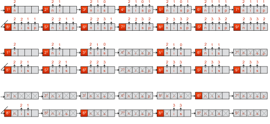
Figure 24: Execution trace of $P$ in Example 10.5 and of the static slice and of their projection.

The formal framework proposed in [Binkley et al. (2006a), Binkley et al. (2006b)] represents different forms of slicing by means of a $(\sqsubseteq,{\mathcal{E}})$ pair: a syntactic preorder, and a function from slicing criteria to semantic equivalences. The preorder fixes a syntactic relation between the program and its slices. In traditional slicing, slices are obtained from the original program by removing zero or more statements. This preorder is called traditional syntactic ordering, simply denoted by $\sqsubseteq$, and it is defined as follows: $Q\sqsubseteq P\Leftrightarrow\mathbb{L}_{Q}\subseteq\mathbb{L}_{P}$ The second component ${\mathcal{E}}$ fixes the semantic constraints that a subprogram has to respect in order to be a slice of the original program. As we have seen before, the equivalence relation is uniquely determined by the chosen slicing criterion determining also a specific form of slicing. This way, Binkley et al. are able to characterize eight forms of non-$\mathtt{SIM}$ slicing, and twelve forms of $\mathtt{SIM}$ slicing.

Finally, this framework is used to formally compare the different notions of slicing. First of all, it is defined a binary relation on slicing criteria $\rightarrow$ [Binkley et al. (2006a)]: Let and

(2)

At this point, we say that a form of slicing $(\sqsubseteq,{\mathcal{E}}^{1})$ is weaker than $(\sqsubseteq,{\mathcal{E}}^{2})$ w.r.t. $\rightarrow$ iff $\forall$, slicing criteria such that , and $\forall P,Q$, if $Q$ is a slice of $P$ w.r.t. $(\sqsubseteq,\mathcal{E}^{2}($, then $Q$ is a slice of $P$ w.r.t. $(\sqsubseteq,\mathcal{E}^{1}($ as well. In this case we say that $(\sqsubseteq,\mathcal{E}^{1})$ subsumes $(\sqsubseteq,\mathcal{E}^{2})$.

Figure 25: Given two forms $A$ and $B$, both (non-)$\mathtt{SIM}$., $A$ is weaker than $B$ if $A$ is connected to $B$ by a solid line and it is below $B$. If $A$ is non-$\mathtt{SIM}$. and $B$ is $\mathtt{SIM}$., then $A$ is weaker than $B$ if $A$ is connected to $B$ by a dotted line and it is to the left of $B$.

Following this definition, Binkley et al. show that all forms of slicing introduced in [Binkley et al. (2006a)] are comparable in the way shown in Figure 25, where the symbols ${\mathcal{S}}$, ${\mathcal{C}}$, ${\mathcal{D}}$, ${\mathcal{S}}{\mathcal{S}}$, ${\mathcal{S}}{\mathcal{C}}$ and ${\mathcal{S}}{\mathcal{D}}$ represent static, conditioned, dynamic, static $\mathtt{SIM}$, conditioned $\mathtt{SIM}$ and dynamic $\mathtt{SIM}$ types of slicing, respectively. Subscripts $i$, $\mathtt{KL}$ and $\mathtt{KL}i$ represent $\mathtt{IC}$, $\mathtt{KL}$ and $\mathtt{KL}i$ forms of slicing, respectively; the absence of subscripts denotes the standard forms of slicing. In Figure 25 we explicitly provide both the hierarchy concerning $\mathtt{SIM}$ and non-$\mathtt{SIM}$ forms of conditioned slicing constructed in [Binkley et al. (2006a)].

References

- Amtoft and Banerjee (2007) Amtoft, T. and Banerjee, A. 2007. A logic for information flow analysis with an application to forward slicing of simple imperative programs. Science of Computer Programming 64, 1, 3–28.
- Barros et al. (2010) Barros, J. B., da Cruz, D., Henriques, P. R., and Pinto, J. S. 2010. Assertion-based slicing and slice graphs. In Proceedings of the 2010 8th IEEE International Conference on Software Engineering and Formal Methods. SEFM ’10. IEEE Computer Society, Washington, DC, USA, 93–102.
- Bijlsma and Nederpelt (1998) Bijlsma, A. and Nederpelt, R. 1998. Dijkstra-Scholten predicate calculus : concepts and misconceptions. Acta Informatica 35, 12, 1007–1036.
- Binkley et al. (2006a) Binkley, D., Danicic, S., Gyimóthy, T., Harman, M., Kiss, A., and Korel, B. 2006a. A formalisation of the relationship between forms of program slicing. Science of Computer Programming 62, 3, 228–252.
- Binkley et al. (2006b) Binkley, D., Danicic, S., Gyimóthy, T., Harman, M., Kiss, A., and Korel, B. 2006b. Theoretical foundations of dynamic program slicing. Theoretical Computer Science 360, 1, 23–41.