An empirical model to form and evolve galaxies in dark matter halos

Abstract

Based on the star formation histories (SFH) of galaxies in halos of different masses, we develop an empirical model to grow galaxies in dark mattet halos. This model has very few ingredients, any of which can be associated to observational data and thus be efficiently assessed. By applying this model to a very high resolution cosmological $N$-body simulation, we predict a number of galaxy properties that are a very good match to relevant observational data. Namely, for both centrals and satellites, the galaxy stellar mass function (SMF) up to redshift $z\simeq 4$ and the conditional stellar mass functions (CSMF) in the local universe are in good agreement with observations. In addition, the 2-point correlation is well predicted in the different stellar mass ranges explored by our model. Furthermore, after applying stellar population synthesis models to our stellar composition as a function of redshift, we find that the luminosity functions in ${}^{0.1}u$, ${}^{0.1}g$, ${}^{0.1}r$, ${}^{0.1}i$ and ${}^{0.1}z$ bands agree quite well with the SDSS observational results down to an absolute magnitude at about -17.0. The SDSS conditional luminosity functions (CLF) itself is predicted well. Finally, the cold gas is derived from the star formation rate (SFR) to predict the HI gas mass within each mock galaxy. We find a remarkably good match to observed HI-to-stellar mass ratios. These features ensure that such galaxy/gas catalogs can be used to generate reliable mock redshift surveys.

1 Introduction

Galaxies are thought to form and evolve in cold dark matter (CDM) halos, however, our understanding of the galaxy formation mechanisms and the interaction between baryons and dark matter are still quite poor, especially quantitatively (see Mo et al. 2010, for a detailed review). Within hydrodynamic cosmological simulations, the evolution of the gas component is described on top of the dark matter, with extensive implementation of cooling, star formation and feedback processes. Such detailed implementation of galaxy formation within a cosmological framework requires vast computational time and resources (Springel et al. 2005).

However the formation of dark matter halos can be easily derived and interpreted, such merger trees can be derived directly from $N$-body simulations, or through Monte Carlo methods. Within those trees, sub-grid models can be applied on the scale of DM halos themselves. Such models are referred as semi-analytic models (hereafter SAM), and provide the means to test galaxy formation models at a much lower computational cost (Cattaneo et al. 2007).

In SAMs, some simple equations describing the underlying physical ingredients regarding the accretion and cooling of gas, star formation etc…, are connected to the dark matter halo properties, so that the baryons can evolve within the dark matter halos merger trees. The related free parameters in these equations are tuned to statistically match some physical properties of observed galaxies.

The basic principles of modern SAMs were first introduced by White & Frenk (1991). Consequently numerous authors participated in the studies of such models and made great progresses (e.g. Kauffmann et al. 1993; Mo et al. 1998; Somerville & Primack 1999; Cole et al. 2000; De Lucia et al. 2004; Kang et al. 2005; Croton et al. 2006; Bower et al. 2006; Monaco et al. 2007; Guo et al. 2011). Through the steerable parameters, SAM has reproduced many statistical properties of large galaxy samples in the local universe such as luminosity functions, galactic stellar mass functions, correlation functions, Tull-Fisher relations, metallicity-stellar mass relations, black hole-bulge mass relations and color-magnitude relations. However, the main shortcoming of SAMs is that there are too many free parameters and degeneracies. Despite the successes of these galaxy formation models, the sub-grid physics is still poorly understood (Benson 2012). By tuning the free parameters, the SAM prediction could match some of the observed galaxy properties in consideration, especially in the local universe. But none of the current SAMs can match the low and high redshift data simultaneously (Somerville et al. 2012). Traditionally, parameters are preferably set without providing a clear statistical measure of success for a combination of observed galaxy properties.

As a SAM cost much less computation time than a full hydrodynamical galaxy formation simulation, one is allowed to explore a wide range of parameter space in acceptable time interval. To better constrain the SAM parameters, Monte Carlo Markov Chains (MCMC) method has been applied to SAMs in recent years. The first paper that incorporated MCMC into SAM is Kampakoglou et al. (2008), which used the star formation rate and metallicity as model constraint. Some other SAM groups also have developed their own models associated with the MCMC method (e.g. Henriques et al. 2009, 2013;Benson & Bower 2010; Bower et al. 2010; Lu et al. 2011, 2012; Mutch et al. 2013). The details of MCMC are beyond the aims of this paper, we refer the readers to these relevant literatures (Press et al. 2007; Trotta 2008).

As pointed out in Benson & Bower (2010), our understanding of galaxy formation is far from complete. SAMs should not be thought of as attempts to provide a final theory of galaxy formation, but instead to provide a mean by which new ideas and insights may be tested and by which quantitative and observationally comparable predictions may be extracted in order to test current theories. Because of the large number of free parameters, new ideas and sights relevant with the sub-grid physics may often bring new degeneracies with increased complexity and uncertainties to the model either traditional SAM or MCMC. In general, if we take a step back from SAMs, we find that the largest part of the parameters and uncertainties are related to the sub-grid physics implemented for the gas. Focussing the model on the formation and evolution of the stars within dark matter halos, the vast majority of the uncertainties in SAM related with the gas component will be reduced.

Understanding the relation between dark matter halos and galaxies is a vital step to model galaxy formation and evolution in dark matter halos. In recent years, we have seen drastic progress in establishing the connection between galaxies and dark matter halos, such as the halo occupation distribution (HOD) models (e.g. Jing et al. 1998, Berlind & Weinberg 2002, Zehavi et al. 2005, Foucaud et al. 2010, Watson et al. 2011, Wake et al. 2012, Leauthaud et al. 2012), and the closely related conditional stellar mass (or luminosity) function models(Yang et al. 2003, van den Bosch et al. 2003, Conroy et al. 2006, van den Bosch et al. 2007, Yang et al. 2009, Yang et al. 2012, Rodríguez-Puebla et al. 2015). The former make use of the clustering of galaxies to constrain the probability of finding $N$ galaxies in a halo of mass $M$. While the latter make use of both clustering and luminosity(stellar mass) functions to constrain the probability of finding galaxies with given luminosity (or stellar mass) in a halo of mass $M$. In a recent study, Yang et al. (2012)(hereafter Y12) proposed a self-consistent model properly taking into account (1) the evolution of stellar-to-halo mass relation of central galaxies; (2) the accretion and subsequent evolution of satellite galaxies. Based on the host halo and subhalo accretion models provided in Zhao et al. (2009) and Yang et al. (2011), Y12 obtained the conditional stellar mass functions (CSMFs) for both central and satellite galaxies as functions of redshift. Based on the mass assembly histories of central galaxies, the amount of accreted satellite galaxies and the fraction of surviving satellite galaxies constrained in Y12, we obtained the star formation histories (SFH) of central galaxies in halos of different masses (Yang et al. 2013). Similar SFH models were also proposed based on $N$-body or Monte Carlo merger trees (e.g., Moster et al. 2013; Behroozi et al. 2013; Lu et al. 2014). These SFH maps give us the opportunity to grow galaxies in $N$-body simulations without the need to model the complicated gas physics. In those models referred as empirical model (EM) of galaxy formation, the growth of galaxies is statistically constrained using observational data.

This paper is organized as follows. In section 2, we describe in detail our simulation data and EM model. In section 3, we show our model predictions associated with the stellar masses of galaxies. The model predictions related with the luminosity and HI gas components are presented in sections 4. Finally, in section 5, we make our conclusions and discuss the applications of our model and the galaxy catalog thus constructed.

2 Simulation and our empirical model

2.1 The simulation

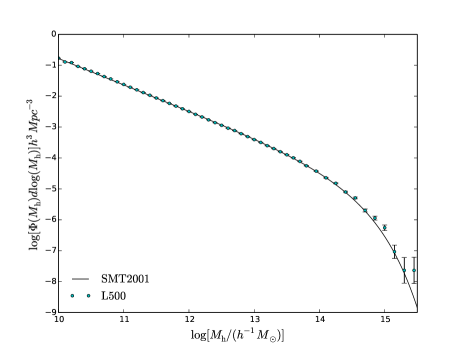
Figure 1: Halo mass functions of the simulation. The black curve and cyan circles represent respectively the Sheth et al. (2001) (SMT2001) analytic prediction and data extracted from the L500 simulation.

Similar to the SAMs, our EM also starts from dark matter halo merger trees. In this study we use dark matter halo merger trees extracted from a high resolution $N$-body simulation. The simulation describes the evolution of the phase-space distribution of $3072^{3}$ dark matter particles in a periodic box of $500\>h^{-1}{\rm{Mpc}}$ on a side. It was carried out in the Center for High Performance Computing, Shanghai Jiao Tong University. This simulation, hereby referred as L500, was run with L-GADGET, a memory-optimized version of GADGET2 (Springel et al. 2005). The cosmological parameters adopted by this simulation are consistent with WMAP9 results as follows: $\Omega_{\rm m}=0.282$, $\Omega_{\Lambda}=0.718$, $\Omega_{\rm b}=0.046$, $n_{\rm s}=0.965$, $h=H_{0}/(100\>{\rm km}\,{\rm s}^{-1}\,{\rm Mpc}^{-1})=0.697$ and $\sigma_{8}=0.817$ (Hinshaw et al. 2013). The particle masses and softening lengths are, respectively, $3.3747\times 10^{8}\>h^{-1}\rm M_{\odot}$ and $3.5h^{-1}\rm kpc$. The simulation is started at redshift 100 and has 100 outputs from z=19, equally spaced in $\log$ (1 + z).

Dark matter halos were first identified by the friends-of-friends(FOF) algorithm with linking length of $0.2$ times the mean particle separation and containing at least $20$ particles. The corresponding dark matter halo mass function (MF) of this simulation at redshift $z=0$ is represented by cyan circles in Fig. 1, while the black curve corresponds to the analytic model prediction by Sheth et al. (2001)(SMT2001). The halo mass function of this simulation is in good agreement with the analytic model prediction in the related mass ranges.

Based on halos at different outputs, halo merger trees were constructed Lacey & Cole (1993). We first use the SUNFIND algorithm (Springel et al. 2001) to identify the bound substructures within the FOF halos or FOF groups. In a FOF group, the most massive substructure is defined as main halo and the other substructures are defined as subhalos. Each particle contained in a given subhalo or main halo is assigned a weight which decreases with the binding energy. We then find all main halos and subhalos in the subsequent snapshot that contain some of its particles. The descendant of any (sub)halo is chosen as the one with the highest weighted count of common particles. This criteria can be understood as a weighed maximum shared merit function (see Springel et al. 2005 for more details). Note that, for some small halos, the tracks of which are temporarily lost in subsequent snapshot, we skip one snapshot in finding their descendants. These descendants are called “non-direct descendant”.

2.2 The empirical model of galaxy formation

Unlike any SAM where each halo initially gets a lump of hot gas to be eventually turned into a galaxy (Baugh 2006), our EM starts with stars. Here we make use of the SFH map of dark matter halos obtained by Yang et al. (2013) to grow galaxies. In our EM of galaxy formation, central and satellite galaxies are assumed to be located at the center of the main halos and subhalos respectively. Their velocities are assigned using those of the main halos and subhalos. For those satellite galaxies whose subhalos are disrupted, (e. g. orphan galaxies) the host halo is populated according to its NFW profile. Their velocities are assigned according to the halo velocity combined with the velocity dispersion (see Yang et al. 2004 for the details of such an assignment).

Apart from the obvious issue of positioning mock galaxies, we have to implement the stellar mass evolution. For central and satellite galaxies, stellar mass $M_{\star,c}(t_{2})$ at a time $t_{2}$ is derived by adding to the stellar mass $M_{\star,c}(t_{1})$ at a time $t_{1}$ the contribution from star formation $\Delta M_{\star,c}(t_{1})$ and disrupted satellites $\Delta M_{\star,dis}(t_{1})$ as follows:

$$M_{\star}(t_{2})=M_{\star}(t_{1})+\Delta M_{\star}(t_{1},t_{2})+\Delta M_{\star,dis}(t_{1},t_{2})$$ (1)

Obviously before implementing these models, the galaxies have to be seeded. For each halo and subhalo, we follow the merger tree back in time to determine the earliest time output (at $t_{\rm min}$) when it was identified as a halo (at least 20 particles). Then a seed galaxy with initial stellar mass $M_{\star}(t_{\rm min})$ is assigned to this halo at the beginning redshift. Here the stellar mass is assigned according to the central-host halo mass relation obtained by Yang et al. (2012), taking into account the cosmology of our simulations. We note that only halos with direct descendants are seeded.

2.2.1 Star formation of central galaxies

We first model the growth of central galaxies that are associated with the host (main) halos. Listed below are the details.

• In order to integrate the contribution of star formation between snapshots corresponding to times $t_{1}$ and $t_{2}=t_{1}+\Delta T$, we increase the time resolution by defining smaller timesteps $\Delta t=\Delta T/N$. Here we choose $N=5$, since greater values have very limited impact on the results. We also assume that the SFR is constant during any time step $\Delta t$.

• Then we estimate ${\dot{M}}_{\star}(t)$ the SFR of central galaxy at time $t$ in a halo with mass $M_{\rm h}$. As shown in Yang et al. (2013), the distribution of SFR of central galaxies have quite large scatters around the median values and show quite prominent bimodal features. To partly take into account these scatters, for each timestep $\Delta t$, the star formation rate ${\dot{M}}_{\star}(t)$ is drawn from a lognormal distribution of mean ${\dot{M}}_{\star,0}(t)$ and dispersion $\sigma$. So the SFR of central galaxies is indeed set as:

  $$\log{\dot{M}}_{\star}(t)=\log{\dot{M}}_{\star,0}(t)+\sigma\cdot N_{\rm gasdev}\,,$$ (2)

  where ${\dot{M}}_{\star,0}(t)$ is the median SFR predicted by Yang et al. (2013) and $N_{\rm gasdev}$ is a random number generated using the code of Numerical Recipe(Press et al. 2007). Here we adopt a $\sigma=0.3$ lognormal scatter as suggested in Yang et al. (2013).

• The stellar mass formed between the snapshots, $\Delta M_{\star}(t_{1},t_{2})$ is determined as:

  $$\Delta M_{\star}(t_{1},t_{2})=\sum_{t=t_{1}}^{t=t_{2}}{\dot{M}}_{\star}(t)\Delta t\,.$$ (3)

2.2.2 Star formation of satellite galaxies

After focussing on the growth of central galaxies, we need to focus on the satellite galaxies. We start by modeling their growth while they are still associated to subhalos. Once the host halo enters a bigger one and becomes a subhalo, the SFR of the new satellite is expected to decline as a function of time due to the stripping effect, etc. Here we use the star formation model of satellite galaxy proposed by Lu et al. (2014) to construct their star formation history. A simple $\tau$ model has been adopted to describe the star formation rate decline in Lu et al. (2014) as follows:

$${\dot{M}}_{\star,{\rm sat}}(t)={\dot{M}}_{\star}(t_{a})\exp\left(-\frac{t-t_{a}}{\tau_{\rm sat}}\right)\,,$$ (4)

where $t_{a}$ is the time when the galaxy is accreted into its host to become a satellite and ${\dot{M}}_{\star}(t_{a})$ the corresponding SFR. $\tau_{\rm sat}$ is the exponential decay time scale characterizing the decline of the star formation for a galaxy of stellar mass $M_{\star}$. We adopt the following model of the characteristic time

$$\tau_{\rm sat}=\tau_{\rm sat,0}\exp\left(-\frac{M_{\star}}{M_{\star,c}}\right)\,,$$ (5)

where $\tau_{\rm sat,0}$ is the time for a galaxy with a stellar mass of $M_{\star,c}$. The values $\tau_{\rm sat,0}$ and $M_{\star,c}$ used in our model are the best fit values of MODEL III in Lu et al. (2014) with $\log(H_{0}\tau_{\rm sat,0})=-1.37$ and $\log M_{\star,c}=-1.4$.

The growth of the satellite stellar mass is thus becomes:

$$\Delta M_{\star,sat}(t_{1},t_{2})={\dot{M}}_{\star}(t_{a})\exp\left(-\frac{t_{2}-t_{a}}{\tau_{\rm sat}}\right)\cdot\Delta T$$ (6)

2.2.3 Merging and stripping of satellite galaxies

Apart from the in situ star formation, another important process in our model is the merging and stripping of satellite galaxies. The merging process has been studied by many people through hydrodynamical simulation (e.g. Zentner et al. 2005; Boylan-Kolchin et al. 2008; Jiang et al. 2008). Here we assume that the satellite galaxies orbiting within a dark matter halo may experience dynamical friction and will eventually be disrupted, while only a small fraction of stars are finally merged with center galaxy of the halo.

So when a satellite cannot be associated with a subhalo, we use a delayed merger scheme where the satellite coalless with the central after the dynamical friction timescale described in the fitting formula of Jiang et al. (2008):

$$T_{\mathrm{dyn}}=1.4188\frac{r_{\rm c}M_{\rm h}}{v_{\rm c}M_{\rm sub}}\frac{1}{\ln(1+\frac{M_{\rm h}}{M_{\rm sub}})}\,,$$ (7)

where $M_{\rm sub}$ and $M_{\rm h}$ are the respective halo masses associated to satellite and central galaxies, at the timestep a satellite galaxy was last found in a subhalo. This formula is valid for a small satellite of halo mass $M_{\rm sub}$ orbiting at a radius $r_{\mathrm{c}}$ in a halo of circular velocity $v_{\mathrm{c}}$. As the satellite galaxy was last found in a subhalo is disrupted after $\Delta t=T_{\mathrm{dyn}}$, we transfer a fraction of its stellar mass to the central galaxy. So that tha contribution of disrupted satellite follows

$$\Delta M_{\star,dis}(t_{1},t_{2})=f_{\mathrm{merger}}\sum M_{\star,sat}(t_{\mathrm{sat}})\,,$$ (8)

where $M_{\star,sat}(t_{sat})$ is stellar mass of the in-falling satellite a determined when it was last found in a subhalo at $t_{\mathrm{sat}}$ with $t_{sat}+T_{\mathrm{dyn}}\leq t_{2}$. $f_{merger}$ is fraction of the satellite galaxy stellar mass merged into central galaxy. Here $f_{\mathrm{merger}}=0.13$ is set to the best fit value of MODEL III in Lu et al. (2014).

2.2.4 Passive evolution of galaxies

Finally, we take into account the passive evolution of both central and satellite galaxies. As we have the stellar mass composition of each galaxy as a function of time, the final stellar mass is determined as:

$$M_{\star}(t_{0})=M_{\star}(t_{\rm min})\cdot f_{\rm passive}(t_{0}-t_{\rm min})+\sum_{t=t_{\rm min}}^{t=t_{0}}\Delta{M}_{\star}(t)\cdot f_{\rm passive}(t_{0}-t)\,,$$ (9)

where $f_{\rm passive}(t)$ is the mass fraction of stars remaining at time $t$ after the formation. We obtained $f_{\rm passive}(t)$ from Bruzual & Charlot (2003), courtesy of Stephane Charlot (private communication).

2.3 Other star formation history models

There have been many other star formation history models proposed in recent years (e.g. Conroy & Wechsler 2009, Behroozi et al. 2013). Here we make use of the model constrained by Lu et al. (2014), in order to further test our empirical model. This model is similar in a sense that it consists on predicting SFR within halos and subhalos to build galaxies. In the larger part of the result section, the properties of the central and satellite galaxies are compared to our fiducial EM predictions.

Lu et al. (2014) (hereafter Lu14) developed an empirical approach to describe the star formation history model of central galaxies and satellite galaxies. They assumed an analytic formula for the SFH of central galaxies with a few free parameters. The galaxies grow in dark matter halos based on the halo merger trees generated by Extended Press-Schechter (EPS: Bond et al. 1991; Bower 1991) formalism and Monte Carlo method. With different observation constraint, they got four different empirical models. Here we only pick Model III in Lu14 to compare with our model. In Lu14, the star formation rate of central galaxies can be written as follows:

$${\dot{M}}_{\star}={\cal E}\frac{f_{B}M_{\rm vir}}{\tau_{0}}\left(1+z\right)^{\kappa}(X+1)^{\alpha}\left(\frac{X+\mathcal{R}}{X+1}\right)^{\beta}\left(\frac{X}{X+\mathcal{R}}\right)^{\gamma}\,,$$ (10)

where ${\cal E}$ is an overall efficiency; $f_{B}$ is the cosmic baryonic mass fraction; $\tau_{0}$ is a dynamic timescale of the halos at the present day, set to be $\tau_{0}\equiv 1/(10H_{0})$; and $\kappa$ is fixed to be ${3/2}$ so that $\tau_{0}/(1+z)^{3/2}$ is roughly the dynamical timescale at redshift $z$. The quantity $X$ is defined to be $X\equiv M_{\rm vir}/M_{\rm c}$, where $M_{\rm c}$ is a characteristic mass and $\mathcal{R}$ is a positive number that is smaller than $1$. For the star formation rate of satellite galaxies, the related formula is already provided in Eq. 4.

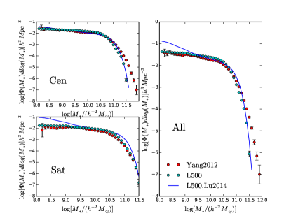
Figure 2: The upper left, lower left and right panels show the galaxy SMFs for central, satellite and all galaxies, respectively. In each panel, the red filled circles with error bars are the galaxy stellar mass function of SDSS DR7 obtained by Yang et al. (2012). The cyan circles with error bars are our fiducial EM results based on L500 simulation. The blue curves are the simular results but based on SFH model of Lu et al. (2014). The error bars of our EM are calculated using 500 bootstrap re-samplings.

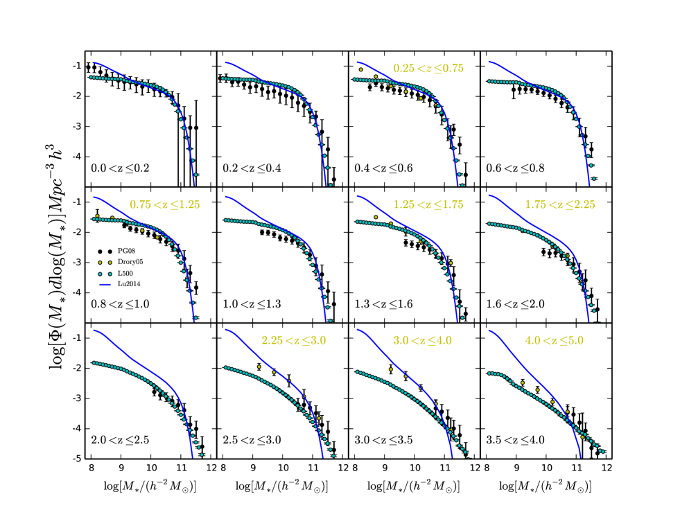
Figure 3: Stellar mass function of galaxies at different redshift bins as indicated in each panel. In all panel we compare our EM prediction(cyan filled circles) and the Lu14 (blue curve) predictions applied to the L500 simulation, to the Spitzer measurements (black circles) published in Pérez-González et al. (2008) (PG08). The redshift selection is indicated in black. We also add results obtained by Drory et al. (2005) (Drory05), in similar redshift ranges (indicated in yellow for the relevant panels). are results from the Spitzer by Pérez-González et al. (2008) (PG08). The error bars of our EM are calculated using 500 bootstrap re-samplings.

3 The stellar mass properties of galaxies

In order to check the performance of our EM for galaxy formation, we check the stellar mass function (SMF) and the two point correlation function (2PCF) of galaxies, and compare them to observational measurements. The related observational measurements are the SMFs at different redshifts (Yang et al. 2012; Pérez-González et al. 2008, hereafter PG08; Drory et al. 2005, hereafter Drory05), the CSMFs at low redshift (Yang et al. 2012) and the 2PCFs for galaxies in different stellar mass bins.

3.1 SMFs of galaxies at different redshifts

The first set of observational measurements are the stellar mass functions of galaxies at redshift $z=0.0$ which are shown in Fig. 2 for all (right panel), central (upper-left panel) and satellite (low-left panel) galaxies, respectively. The red circles with error-bars indicate the observational data obtained from SDSS DR7 by Yang et al. (2012). Cyan circles with error bars are the results of our model applied the halo merger trees of the L500 simulation. Meanwhile, blue curves are obtained using the Lu14 SFH model on the same trees.

From the upper-left panel of Fig. 2, it is clear that for central galaxies the results of our model show an excellent agreement with observational data within a large stellar mass range ($\log M_{\ast}\sim 8.1-11.0$). However, in high mass range ($\log M_{\ast}\ga 11.0$), we somewhat underestimate the stellar mass function. This discrepancy is probably caused by the fact that in our model, we used the median SFH to grow galaxies in dark matter halos. However, in reality scatter of SFHs of high mass central galaxies may be larger and depend on their large scale environment. In addition, in our model we did not take into account the major mergers of galaxies, where only $f_{\rm merger}=0.13$ portion of stripped satellite galaxies can be accreted to the central galaxies. For the SFH models of Lu14, the results are very similar with our fiducial ones.

For the satellite galaxies, as shown in the lower-left panel of Fig. 2, our fiducial EM reproduces the overall SMFs quite well. However, a slight deviation (over prediction) is seen at middle mass range ($\log M_{\ast}\sim 10.4-10.9$). In these satellite galaxies either the SFH modelled by Eq. 4 is somewhat too strong, or the stripping and disruption of satellite modelled by Eq. 7 is not efficient enough. As for Lu14 model, it does not match that well with the SDSS observations, especially in the low mass range ($\log M_{\ast}\sim 8.0-9.5$). And in high mass range($\log M_{\ast}\sim 11.0-11.5$), it over predicts the mass function. Nevertheless, as Lu14 model itself is intended to reproduce the much steeper faint end slope of the luminosity function, especially for satellite galaxies, such differences are expected.

The right panel of Fig. 2 shows the SMF of all galaxies which include central galaxies and satellite galaxies. The results of our fiducial EM in general agree with the observational data, with slight discrepancies at the high mass range ($\log M_{\ast}\ga 11.0$) mainly contributed by centrals, and at middle mass range ($\log M_{\ast}\sim 10.4-10.9$) mainly contributed by satellites. The Lu14 model show a larger discrepancy at low mass range($\log M_{\ast}\sim 8.0-9.5$) which is caused by the satellite components.

Next, we check the stellar mass functions of galaxies at higher redshifts. Shown in Fig. 3 are SMFs of galaxies at different redshift bins as indicated in each panel. In these higher redshift bins, in order to mimics the typical error in the stellar mass estimation in observations, we add logarithmic scatters to the stellar masses of galaxies as $\sigma_{c}(z)={\rm max}[0.173,0.2z]$ (see Yang et al. 2012 for more detail). The yellow filled circles with error-bars are results obtained by Drory et al. (2005), in which they have combined the data from FORS Deep and from the GOODS/CDFS Fields. The cyan circles with error bars are our EM results based on L500 simulation, while blue curves are the results of Lu14 model based on L500 simulation.

As shown in Fig. 3, in both low and high redshift bins $z<1.0$ and $z>2.0$, the SMFs from our model agree quite well with the observational results. However in the redshift range $1.0<z<2.0$, our model over predicts the SMFs. As seen in the lower-left panel of Fig. 2, this discrepancies might be due to some over prediction of satellite galaxy counts. In comparison, we also show results based on Lu14 model, which present even higher SMFs within the redshift range $1.0<z<2.0$.

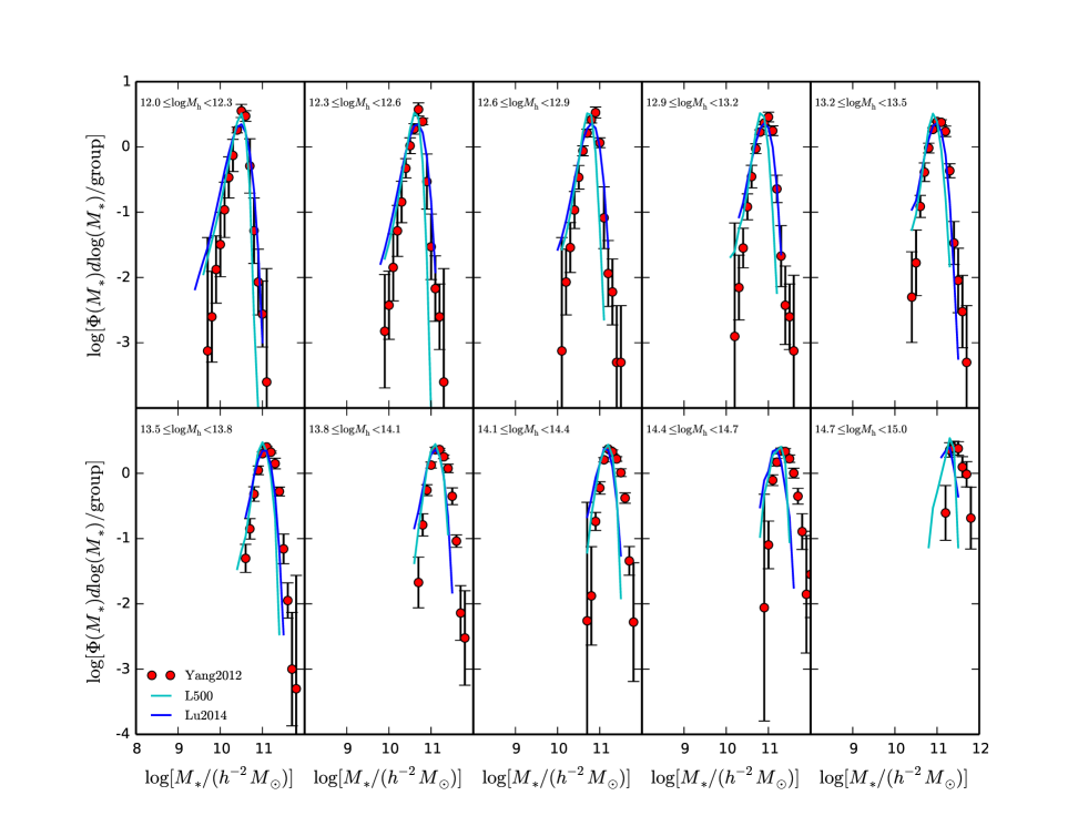
Figure 4: Conditional stellar mass functions (CSMFs) of central galaxies. Different panel corresponds to different halo mass bin as indicated. The cyan solid curves are the CSMFs of our EM, while blue curves are obtained using Lu14 SFH model. Red filled circles with error bars are the CSMFs of SDSS DR7 obtained by Yang et al. (2012).

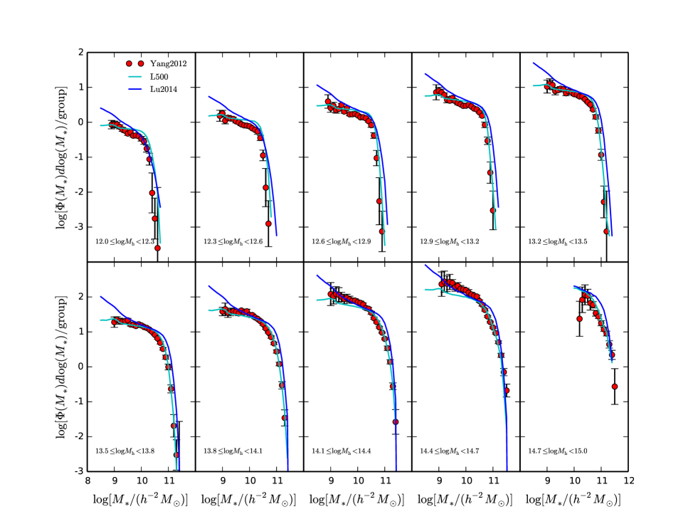
Figure 5: Similar to Fig. 4 but for satellite galaxies.

3.2 CSMFs of galaxies at $z=0$

The conditional stellar mass function (CSMF) $\phi(M_{\ast}|M_{\rm h})$, which describes the average number of galaxies as a function of galaxy stellar mass $M_{\ast}$ that can be formed within halos of mass $M_{\rm h}$, is an important measure that can be used to constrain galaxy formation models. As carried out in Liu et al. (2010) using the CSMFs of satellite galaxies, classical semi-analytical models at that time typically over predicted the satellite components by a factor of two which indicates that either less (or smaller) satellites can be formed, or more satellite galaxies need to be disrupted. Here we compare our model predictions with observational data in Fig. 4 and Fig. 5 for central and satellite galaxies separately.

Based on the SDSS DR7 galaxy group catalog, Yang et al. (2012) obtained the CSMFs of central galaxy and satellite galaxies, which are shown as the red filled circles with error-bars in Fig. 4 and Fig. 5, respectively. The CSMFs from our model are shown as cyan solid curves. Blue curves are the CSMFs obtained from galaxy catalogs constructed using Lu14 model. As shown in Fig. 4, the central galaxy CSMFs of our model and Lu14 model are very similar. Both of them agree well with the observations in halo mass range $12.0\leq\log M_{\rm h}<13.8$ but are slightly under estimated in halo mass range $13.8\leq\log M_{\rm h}<15.0$. As shown in Fig. 5 for satellite galaxies, the CSMFs of our model agree well with the observation in general. There are little deviations in halo mass ranges $12.0\leq\log M_{\rm h}<12.3$, $12.3\leq\log M_{\rm h}<12.6$ and $12.6\leq\log M_{\rm h}<12.9$. In these ranges, our model overestimates the CSMFs at $9.5\leq\log M_{\ast}<10.5$. Thus the over predicted satellite galaxies shown in Fig. 2 are mainly in these Milky Way sized and group sized halos. While in Lu14 model, as seen for the satellite galaxy stellar mass function shown in Fig. 2, the CSMFs in halos of different masses all show an upturn at low mass end.

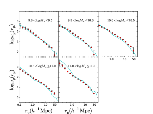
Figure 6: Projected 2PCFs of galaxies in different stellar mass bins as indicated in each panel. Red filled circles with error bars are the 2PCFs of SDSS DR7 obtained by Yang et al. (2012) and cyan curves are our EM results.

3.3 2PCFs of galaxies

The two point correlation function which measures the excess of galaxy pairs as a function of distance is a widely used quantity to describe the clustering properties of galaxies. In terms of galaxy formation, it can be used to constrain the HOD of galaxies (Jing et al. 1998) and to constrain the CLF of galaxies (Yang et al. 2003). Here we compare the model predictions of 2PCFs in our galaxy catalogs to observations.

Fig. 6 shows the projected 2PCFs of galaxies in different stellar mass bins. Our model predictions are shown as the solid curves and the observational data obtained by Yang et al. (2012) from SDSS DR7 are shown as the filled circles with error bars. Our overall model predictions are quite a good match to the observation in the stellar mass range $9.0<\log M_{\ast}<11.0$. However, in the most massive stellar mass bin ($11.0<\log M_{\ast}<11.5$), our model results is higher than the observations for $r_{\rm p}\la 1h^{-1}\rm Mpc$. The too strong clustering at $r_{\rm p}<1\>h^{-1}{\rm{Mpc}}$ for these high mass objects is mainly caused by the fact that due to the insufficient prediction of the central galaxies, the satellite fraction in this mass bin is over predicted (see Fig. 2).

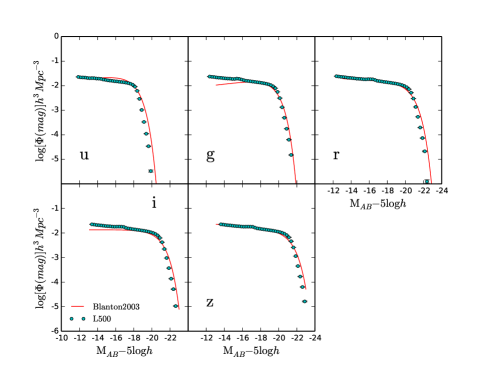
Figure 7: Luminosity functions of galaxies in $u,g,r,i,z$ band at $z=0.1$. The solid curve in each panel is the corresponding best fit Schechter form LF obtained by Blanton et al. (2003) from SDSS DR1.

Figure 8: Luminosity functions of central, satellite and all galaxies in $r$ band in the local universe. Here results are shown for observational measurements (red dots) and our fiducial model predictions (cyan dots), respectively.

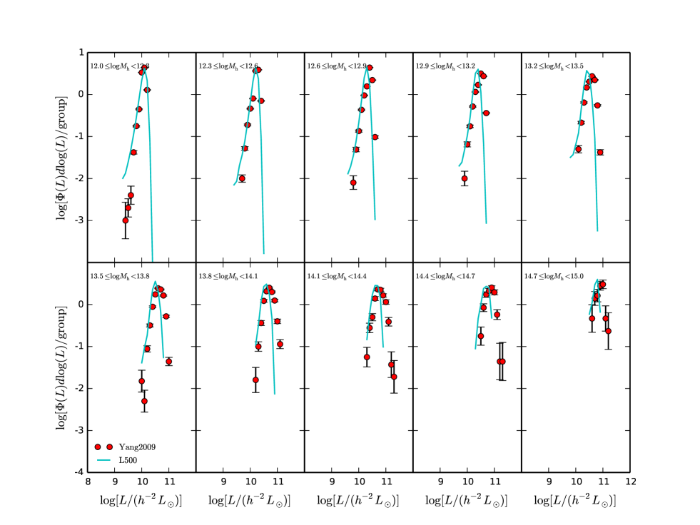
Figure 9: Conditional luminosity functions (CLFs) of central galaxies in halos of different mass bins. Here results are shown for observational measurements (red dots) and our fiducial model predictions (cyan curves), respectively.

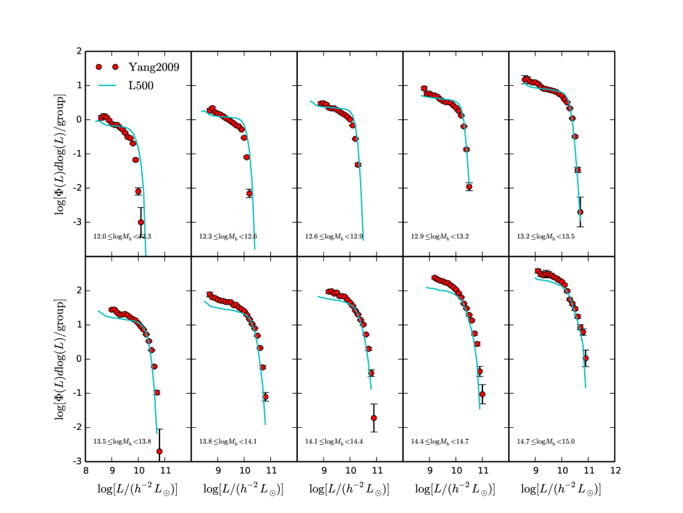
Figure 10: Similar as Fig. 9 but for the satellite galaxies.

4 The luminosity and gas properties of galaxies

Apart from the stellar masses of galaxies, we now turn to the luminosity and gas components of galaxies.

4.1 Luminosities of galaxies in different bands

As detailled in section 2.2, from the halo merger histories derived from the L500 simulation, we model galaxies from a estimation of their sellar mass and SFR as a function of time. We use those information to predict the photometric properties of our model galaxies using the stellar population synthesis model of Bruzual & Charlot (2003) using a Salpeter IMF (Salpeter 1955). Since our model does not include the gas component in galaxies, we cannot directly trace the chemical evolution of the stellar population. To circumvent this problem, we follow the metallicity - stellar mass relation derived in Lu14 from observation of galaxies at all redshifts specified redshift range of ranges. We adopt the mean relation based on the data of Gallazzi et al. (2005), which can roughly be described as

$$\log_{10}Z=\log_{10}Z_{\odot}+\frac{1}{\pi}\tan\left[\frac{\log_{10}(M_{\star}/10^{10}M_{\odot})}{0.4}\right]-0.3\,.$$ (11)

This observational relation extends down to a stellar mass of $10^{9}M_{\odot}$ and has a scatter of $0.2\,{\rm dex}$ at the massive end and of $0.5\,{\rm dex}$ at the low mass end.

Using the stellar population synthesis model, we can obtain galaxy luminosities in different bands. We show in Fig. 7, the luminosity functions of all galaxies in the five different SDSS bands ($u,g,r,i,z$) at $z=0.1$. For comparison, we also show in each panel the corresponding best Schechter functional LFs fit obtained by Blanton et al. (2003) from SDSS DR1. The observational measurements and corresponding model fitting are roughly limited to absolute magnitude limit ($-16,-16.5,-17,-17.5,-18$) in ($u,g,r,i,z$) bands, respectively. Within these magnitude limits, our model predictions agree with the observational data fairly well with very slight under predictions at the bright ends. Only in $u$-band do we see a pro-eminent deficit of galaxies at $\>{}^{0.1}{\rm M}_{u}-5\log h\sim-16.0$. These behaviors indicate that the stellar compositions as a function of time as derived with our model are on average accurate.

In addition to the LFs of the full galaxy population, we can distinguish the contribution from the centrals and the satellites. Fig. 8 shows the $r$ band luminosity functions of all (right panel), central (upper-left panel) and satellite (low-left panel) galaxies. Our fiducial model predictions are shown as the cyan dots with error bars obtained from 500 bootstrap re-samplings. Red points with error bars are obtained by Yang et al. (2009) but were updated to SDSS DR7. Similar with Fig. 2, our model underestimates the central galaxy luminosity function at high luminosity end ($10.5\la\log L\la 11.0$) and overestimates the satellite galaxy luminosity function in the luminosity range ($10.0\la\log L\la 10.5$).

Similarly to the CSMFs, the conditional luminosity functions(CLFs) describe, as a function of luminosity $L$, the average number of galaxies that reside in dark matter halo of a given mass $M_{h}$. In Fig. 9 the CLFs obtained from our mock catalogs are compared to the observational measurements obtained by Yang et al. (2009)(also updated to SDSS DR7). As one could expect, the performances of CLFs of central galaxies is quite similar to the situation found for the CSMFs in Fig. 4. The central galaxy CLFs of our model agree well with the observational results in the $12.0\leq\log M_{\rm h}<13.5$ halo mass range still there is some discrepancy for $13.5\leq\log M_{\rm h}<15.0$.

As for the satellite galaxies shown in Fig. 10, the situation is somewhat different with respect to the CSMFs. Our model matches well with observations in $12.9\leq\log M_{\rm h}<13.8$, while underestimate the number of satellite galaxies at the low luminosity end in high mass halos $13.8\leq\log M_{\rm h}<15.0$. These discrepancies are highly interesting as they differ from the one we found for the CSMFs (Fig 5), as it indicates that the colors of these galaxies are not entirely properly modelled.

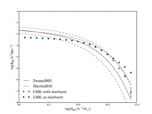
Figure 11: The HI mass functions: green dots are our fiducial model predictions, while cyan dots are the model predictions that taken into account the starburst. The black solid line shows the best fit observational results obtained by Zwaan et al. (2005) with dashed lines indicate its $\pm 1\sigma$ scatter. Magenta curve is the observational fitting formula obtained by Martin et al. (2010).

Figure 12: The HI-to-stellar mass ratios as a function of galaxy stellar mass. Here red points are data from GASS (Catinella et al. 2013) survey. Red curves are the median and 68% confidence range of the ratio in the GASS sample. Green and cyan curves represent the median and 68% confidence range of our fiducial and star-burst model predictions, respectively.

4.2 HI masses of galaxies

Although our EM is limited to model the star components of galaxies, we can estimate the gas components within the galaxies. Here we focus on the cold gas that are associated with the star formation(Schmidt 1959). The star formation law most widely implemented in SAM was proposed by Kennicutt (1998) as follows:

$$\Sigma_{\mathrm{SFR}} = (2.5\pm 0.7)\times 10^{-4}$$ (12)

$$(\frac{\Sigma_{\mathrm{gas}}}{1\>{\rm M_{\odot}}\mathrm{pc}^{-2}})^{1.4\pm 0.15}\>{\rm M_{\odot}}\mathrm{yr}^{-1}\mathrm{kpc}^{-2}\,,$$

where $\Sigma_{\mathrm{SFR}}$ and $\Sigma_{\mathrm{gas}}$ are the surface densities star formation and gas, respectively.

In this paper, we use the model proposed in Fu et al. (2010) to estimate the cold gas within our galaxies. This method consists in following the build-up of stars and gas within a fixed set of 30 radial “rings”. The radius of each ring is given by the geometric series

$$r_{i} = 0.5\times 1.2^{i}[h^{-1}\rm{kpc}](i=1,2...30).$$ (13)

According to Mo et al. (1998), the cold gas is distributed exponentially with surface density profile

$$\Sigma_{\mathrm{gas}}(r) = \Sigma_{\mathrm{gas}}^{\mathrm{0}}\exp(-r/r_{\mathrm{d}})\,,$$ (14)

where $r_{\mathrm{d}}$ is the scale length of the galaxy, and $\Sigma_{\mathrm{gas}}^{\mathrm{0}}$ is given by $\Sigma_{\mathrm{gas}}^{\mathrm{0}}=m_{\mathrm{gas}}/(2\pi r_{\mathrm{d}}^{\mathrm{2}})$.

With the above ingredients, we are able to predict the total amount of cold gas associated to each galaxy. However, observationally, we only have a relatively good estimate of HI mass in the local universe. Here we calculate HI masses associated to galaxies by assuming a constant ${\rm H}_{2}/{\rm HI}$ ratio of 0.4 and a hydrogen mass fraction $X=0.74$ (Lagos et al. 2011; Baugh et al. 2004; Power et al. 2010). Fig. 11 shows the HI mass function of galaxies in the local universe obtained from our mock galaxy catalog (green dots). For comparison, we also show in Fig. 11, using black curve, the fitting formula of HI mass function obtained by Zwaan et al. (2005) from HIPASS:

$$\Theta(M_{\mathrm{HI}})dM_{\mathrm{HI}}=\left(\frac{M_{\mathrm{HI}}}{M^{\ast}_{\mathrm{HI}}}\right)^{\alpha}\exp\left(-\frac{M_{\mathrm{HI}}}{M^{\ast}_{\mathrm{HI}}}\right)d\left(\frac{M_{\mathrm{HI}}}{M^{\ast}_{\mathrm{HI}}}\right)\,,$$ (15)

where $\alpha=-1.37\pm 0.03$ and $\log(M^{\ast}_{\mathrm{HI}})/\>{\rm M_{\odot}}=9.80\pm 0.03h^{-2}_{75}$. Black dashed lines indicate the $\pm 1\sigma$ scatter. An additional observational HI mass function is obtained by Martin et al. (2010) using $1/V_{max}$ method (magenta curve).

Our model only shows a fair agreement to these observational data, even though it under predicts the HI mass function at $\log M_{\rm HI}\la 9.6$ and over predicts the HI mass function at $\log M_{\rm HI}\ga 10.5$. These discrepancies are possibly caused by different factors. The first one am be, of course, the uncertainties in the SFR-cold gas mass ratios. In addition to this, as the SFR in low mass halos have much larger scatters than the ones we adopt here (see Fig. 1 in Yang et al. (2013)), adopting a larger scatter may help to solve the HI mass function deficiency at low mass end. On the massive end of the HI mass function, the difference may be connected to starburst galaxies (with high SFR). However, in reality, starburst is not necessary associated with the largest cold gas component. As Luo et al. (2014) have checked the morphologies of star-burst galaxies (with SFRs 5 time higher than the median for the given stellar mass), and found that more than half of them are associated with gas rich major mergers. To partly take this into account, we adopt the collisional star-burst model proposed by Somerville et al. (2001) used in many SAMs (Somerville et al. 2008; Guo et al. 2011). During the star-burst process, the increased stellar mass of the central galaxy is

$$\delta m_{\mathrm{starburst}} = (m_{\mathrm{gas,\;sat}}+m_{\mathrm{gas,\;cen}})$$ (16)

$$e_{\mathrm{burst}}\left(\frac{m_{\mathrm{sat}}}{m_{\mathrm{cen}}}\right)^{\mathrm{\gamma_{burst}}}\,,$$

where $m_{\mathrm{gas,\;cen}}$ ($m_{\mathrm{gas,\;sat}}$) is the cold gas mass of central (satellite) galaxy, $m_{\mathrm{cen}}$ ($m_{\mathrm{sat}}$) is the sum of stellar mass and cold gas mass of central (satellite) galaxy, $e_{\mathrm{burst}}=0.55$, and $\gamma_{\mathrm{burst}}=0.69$. The values of $e_{\mathrm{burst}}$ and $\gamma_{\mathrm{burst}}$ are determined from isolated galaxy merger simulations performed by Cox et al. (2008). Within our merger trees, we identify these star-burst galaxies and swap their SFRs to the highest ones in similar mass halos. The cold gas for these galaxies are updated using this Eq. 16. We show in Fig. 11 using cyan dots how this starburst implementation successfully corrects the over-estimation of HI mass function at massive end.

Apart from the HI mass functions, we also compare the HI-to-stellar mass ratios of galaxies. Fig. 12 illustrates the HI-to-stellar mass ratio $\log[M_{\rm HI}/M_{\ast}]$ as a function of galaxy stellar mass. Red points are from GASS survey (Catinella et al. 2013) while the red curve represents the median value and red dashed curves indicate the $16^{th}$ and $84^{th}$ percentile ranges of $\log[M_{\rm HI}/M_{\ast}]$. The green solid and dashed curves represent the median and $16^{th}$ and $84^{th}$ percentile ranges of our fiducial model prediction from the L500 simulation. While the cyan curves are obtained from the star-burst variation of the model. We can see that both our models reproduce the average trends of HI-to-stellar mass ratios as a function of stellar mass quite well. But the scatter of the model prediction is smaller than the observation at low masses. We think that this may caused by the relation between star formation rate and cold gas used in our model.

5 Summary

Based on the star formation histories of galaxies in halos of different masses derived by Yang et al. (2013), we an empirical model to study the galaxy formation and evolution. Compared to traditional SAMs, this model has few free parameters, each of which can be associated with the observational data. Applying this model to merger trees derived from $N$-body simulations, we predict several galaxy properties that agree well with the observational data. Our main results can be summarized as follows.

1. At redshift $z=0$, the SMFs of all galaxies agree well with the observation within $8.0<\log M_{\ast}<11.3$ but our estimate is slightly low in high stellar mass end ($11.3<\log M_{\ast}<12.0$).

2. Our SMFs show generally a fair agreement with the observational data at higher redshifts up to 4. While in redshift $1.0<z<2.0$, the SMFs at the low mass end are somewhat over-estimated.

3. At redshift $z=0$, the CSMFs of central galaxies agree well with the observations in the $12.0\leq\log M_{\rm h}<13.8$ halo mass range and somewhat shifted to lower masses in halo mass range $13.8\leq\log M_{\rm h}<15.0$. In the meantime, the CSMFs of satellite galaxies agree quite well with the observations.

4. The projected 2PCFs in different stellar mass bins calculated from our fiducial galaxy catalog can match well the observations. Only in the most massive stellar mass bin the correlation is over predicted at small scales.

5. We can derive from our model LFs in the ${}^{0.1}u$, ${}^{0.1}g$, ${}^{0.1}r$, ${}^{0.1}i$ and ${}^{0.1}z$ bands. They prove to be roughly consistent with the SDSS observational results obtained by Blanton et al. (2003).

6. The central galaxy CLFs of our model agree well with the observational results in halo mass range $12.0\leq\log M_{\rm h}<13.5$, quite similar to the SMFs. However, the satellite galaxy CLFs are somewhat underestimated at faint end in halos with mass $12.9\leq\log M_{\rm h}<13.8$.

7. Our prediction of HI mass function agree with the observational data at roughly $\pm 1\sigma$ level at $\log M_{\rm HI}\ga 9.6$, and somewhat underestimated at lower mass ends.

Our model predicts roughly consistent, although not perfect, stellar mass, luminosity and HI mass components of galaxies. Such a method is a potential tool to study the galaxy formation and evolution as an alternative to SAMs or abundance matching methods. The galaxy and gas catalogs here constructed can be used to construct redshift surveys for future deep surveys.