Simultaneous Identification of Damping Coefficient and Initial Value for PDEs from Boundary Measurement

Abstract

In this paper, the simultaneous identification of damping or anti-damping coefficient and initial value for some PDEs is considered. An identification algorithm is proposed based on the fact that the output of system happens to be decomposed into a product of an exponential function and a periodic function. The former contains information of the damping coefficient, while the latter does not. The convergence and error analysis are also developed. Three examples, namely an anti-stable wave equation with boundary anti-damping, the Schrödinger equation with internal anti-damping, and two connected strings with middle joint anti-damping, are investigated and demonstrated by numerical simulations to show the effectiveness of the proposed algorithm.

Keywords:  Identification; damping coefficient; anti-stable PDEs; anti-damping coefficient.

AMS subject classifications:  35K05, 35R30, 65M32, 65N21, 15A22.

1 Introduction

Let $H$ be a Hilbert space with the inner product $\langle\cdot,\cdot\rangle$ and inner product induced norm $\|\cdot\|$, and let $Y={\mathbb{R}}$ (or ${\mathbb{C}}$). Consider the dynamic system in $H$:

$$\left\{\begin{array}[]{ll}\dot{x}(t)=A(q)x(t),\;x(0)=x_{0},\\ y(t)=Cx(t)+d(t),\end{array}\right.$$ (1.1)

where $A(q):D(A(q))\subset H\rightarrow H$ is the system operator depending on the coefficient $q$, which is assumed to be a generator of $C_{0}$-semigroup $\mathcal{T}_{q}=(T_{q}(t))_{t\in{\mathbb{R}}^{+}}$ on $H$, $C:H\rightarrow Y$ is the admissible observation operator for $\mathcal{T}_{q}$ ([20]), $x_{0}\in H$ is the initial value, and $d(t)$ is the external disturbance.

Various PDE control systems with damping mechanism can be formulated into system (1.1), where $q$ is the damping coefficient. For a physical system, if the damping is produced by material itself that dissipates the energy stored in system, then the system keeps stable. The identification of damping coefficient has been well considered for distributed parameter systems like Kelvin-Voigt viscoelastic damping coefficient in Euler-Bernoulli beam investigated in [4], and a more general theoretical framework for various classes of parameter estimation problems presented in [5]. In these works, the inverse problems are formulated as least square problems and are solved by finite dimensionalization. For more revelent works, we can refer to the monograph [6]. Sometimes, however, the source of instability may arise from the negative damping. One example is the thermoacoustic instability in duct combustion dynamics and the other is the stick-slip instability phenomenon in deep oil drilling, see, for instance, [7] and the references therein. In such cases, the negative damping will result in all the eigenvalues located in the right-half complex plane, and the open-loop plant is hence “anti-stable” (exponentially stable in negative time) and the $q$ in such kind of system is said to be the anti-damping coefficient.

A widely investigated problem in recent years is stabilization for anti-stable systems by imposing feedback controls. A breakthrough on stabilization for an anti-stable wave equation was first reached in [19] where a backstepping transformation is proposed to design the boundary state feedback control. By the backstepping method, [11] generalizes [19] to two connected anti-stable strings with joint anti-damping. Very recently, [12, 13] investigate stabilization for anti-stable wave equation subject to external disturbance coming through the boundary input, where the sliding mode control and active disturbance rejection control technology are employed. It is worth pointing out that in all aforementioned works, the anti-damping coefficients are always supposed to be known.

On the other hand, a few stabilization results for anti-stable systems with unknown anti-damping coefficients are also available. In [16], a full state feedback adaptive control is designed for an anti-stable wave equation. By converting the wave equation into a cascade of two delay elements, an adaptive output feedback control and parameter estimator are designed in [7]. Unfortunately, no convergence of the parameter update law is provided in these works.

It can be seen in [7, 16] that it is the uncertainty of the anti-damping coefficient that leads to complicated design for adaptive control and parameter update law. This comes naturally with the identification of unknown anti-damping coefficient. To the best of our knowledge, there are few studies on this regard. Our focus in the present paper is on simultaneous identification for both anti-damping (or damping) coefficient and initial value for system (1.1), where the coefficient $q$ is assumed to be in a prior parameter set $Q=[\underline{q},\overline{q}]$ ($\underline{q}$ or $\overline{q}$ may be infinity) and the initial value is supposed to be nonzero.

We proceed as follows. In Section 2, we propose an algorithm to identify simultaneously the coefficient and initial value through the measured observation. The system may not suffer from disturbance or it may suffer from general bounded disturbance. In Section 3, a wave equation with anti-damping term in the boundary is discussed. A Schrödinger equation with internal anti-damping term is investigated in Section 4. Section 5 is devoted to coupled strings with middle joint anti-damping. In all these sections, numerical simulations are presented to verify the performance of the proposed algorithms. Some concluding remarks are presented in Section 6.

2 Identification algorithm

Before giving the main results, we introduce the following well known Ingham’s theorem [14, 15, 23] as Lemma 2.1.

Lemma 2.1.

Assume that the strictly increasing sequence $\{\omega_{k}\}_{k\in\mathbb{Z}}$ of real numbers satisfies the gap condtion

$$\omega_{k+1}-\omega_{k}\geq\gamma\quad\mbox{for all}\quad k\in\mathbb{Z},$$ (2.1)

for some $\gamma>0$. Then, for all $T>2\pi/\gamma$, there exist two positive constants $C_{1}$ and $C_{2}$, depending only on $\gamma$ and $T$, such that

$$C_{1}\sum_{k\in\mathbb{Z}}|a_{k}|^{2}\leq\displaystyle\int_{0}^{T}\left|\sum_{k\in\mathbb{Z}}a_{k}e^{i\omega_{k}t}\right|^{2}dt\leq C_{2}\sum_{k\in\mathbb{Z}}|a_{k}|^{2},$$ (2.2)

for every complex sequence $(a_{k})_{k\in\mathbb{Z}}\in\ell^{2}$, where

$$C_{1}=\displaystyle\frac{2T}{\pi}\left(1-\displaystyle\frac{4\pi^{2}}{T^{2}\gamma^{2}}\right),\;C_{2}=\displaystyle\frac{8T}{\pi}\left(1+\displaystyle\frac{4\pi^{2}}{T^{2}\gamma^{2}}\right).$$ (2.3)

To begin with, we suppose that there is no external disturbance in system (1.1), that is,

$$\left\{\begin{array}[]{ll}\dot{x}(t)=A(q)x(t),\;x(0)=x_{0},\\ y(t)=Cx(t).&\end{array}\right.$$ (2.4)

The succeeding Theorem 2.1 indicates that identification of the coefficient $q$ and initial value $x_{0}$ can be achieved exactly simultaneously without error for $A(q)$ with some structure.

Theorem 2.1.

Let $A(q)$ in system (2.4) generate a $C_{0}$-semigroup $\mathcal{T}_{q}=(T_{q}(t))_{t\in{\mathbb{R}}^{+}}$ and suppose that $A(q)$ and $C$ satisfy the following conditions:

(i). $A(q)$ has a compact resolvent and all its eigenvalues $\{\lambda_{n}\}_{n\in{\mathbb{N}}}$ (or $\{\lambda_{n}\}_{n\in\mathbb{Z}}$) admit the following expansion:

$$\lambda_{n}=f(q)+i\mu_{n},\quad\cdots<\mu_{n}<\mu_{n+1}<\cdots,$$ (2.5)

where $f:\;Q\rightarrow{\mathbb{R}}$ is invertible, $\mu_{n}$ is independent of $q$, and there exists an $L>0$ such that

$$\frac{\mu_{n}L}{2\pi}\in\mathbb{Z}\mbox{ for all }n\in{\mathbb{N}}.$$ (2.6)

(ii). The corresponding eigenvectors $\{\phi_{n}\}_{n\in{\mathbb{N}}}$ form a Riesz basis for $H$.

(iii). There exist two positive numbers $\kappa$ and $K$ such that $\kappa\leq|\kappa_{n}|\leq K$ for all $n\in{\mathbb{N}}$, where

$$\kappa_{n}:=C\phi_{n},\quad n\in{\mathbb{N}}.$$ (2.7)

Then both coefficient $q$ and initial value $x_{0}$ can be uniquely determined by the output $y(t),t\in[0,T]$, where $T>2L$. Precisely,

$$q=f^{-1}\left(\displaystyle\frac{1}{L}\ln\displaystyle\frac{\|y\|_{L^{2}(T_{1},T_{2})}}{\|y\|_{L^{2}(T_{1}-L,T_{2}-L)}}\right),$$ (2.8)

for any $L<T_{1}<T_{2}-L$, and

$$x_{0}=\displaystyle\frac{1}{L}\sum_{n\in{\mathbb{N}}}\displaystyle\frac{1}{\kappa_{n}}\left(\int_{0}^{L}y(t)e^{-\lambda_{n}t}dt\right)\phi_{n}.$$ (2.9)

Proof.

Since $\{\phi_{n}\}_{n\in{\mathbb{N}}}$ forms a Riesz basis for $H$, there exists a sequence $\{\psi_{n}\}_{n\in{\mathbb{N}}}$ of eigenvectors of $A(q)^{\ast}$, which is biorthogonal to $\{\phi_{n}\}_{n\in{\mathbb{N}}}$, that is, $\langle\phi_{n},\psi_{m}\rangle=\delta_{nm}$. In this way, we can express the initial value $x_{0}\in H$ as $x_{0}=\sum_{n\in{\mathbb{N}}}\langle x_{0},\psi_{n}\rangle\phi_{n},$ and the solution of system (2.4) as

$$x(t)=T_{q}(t)x_{0}=\sum_{n\in{\mathbb{N}}}e^{\lambda_{n}t}\langle x_{0},\psi_{n}\rangle\phi_{n}.$$ (2.10)

By (2.6), there exists an increasing sequence $\{K_{n}\}\subset\mathbb{Z}$ such that

$$\mu_{n}=\displaystyle\frac{2\pi K_{n}}{L},\;n\in{\mathbb{N}},$$ (2.11)

which implies that $\{\mu_{n}\}$ satisfies the following gap condition

$$\mu_{n+1}-\mu_{n}=\displaystyle\frac{2\pi(K_{n+1}-K_{n})}{L}\geq\displaystyle\frac{2\pi}{L}\triangleq\gamma.$$ (2.12)

In addition, by the assumption that $\{\phi_{n}\}$ forms a Riesz basis for $H$ and $|C\phi_{n}|$ is uniformly bounded with respect to $n$, it follows from Proposition 2 of [8] or Theorem 2 of [9] that $C$ is admissible for $\mathcal{T}_{q}$. So generally, we have

$$y(t)=Cx(t)=\displaystyle\sum_{n\in{\mathbb{N}}}e^{\lambda_{n}t}\langle x_{0},\psi_{n}\rangle C\phi_{n}=e^{f(q)t}\displaystyle\sum_{n\in{\mathbb{N}}}e^{i\mu_{n}t}\langle x_{0},\psi_{n}\rangle C\phi_{n}\triangleq e^{f(q)t}P_{L}(t),$$ (2.13)

where $P_{L}(t)=\sum_{n\in{\mathbb{N}}}e^{i\mu_{n}t}\langle x_{0},\psi_{n}\rangle C\phi_{n}$ is well-defined and it follows from (2.11) that $P_{L}(t)$ is a $Y$-valued function of period $L$. For any $T_{2}-L>T_{1}>L$,

$$\int_{T_{1}}^{T_{2}}\left|y(t)\right|^{2}dt=e^{2f(q)L}\displaystyle\int_{T_{1}-L}^{T_{2}-L}\left|y(t)\right|^{2}dt,$$ (2.14)

that is,

$$\|y\|_{L^{2}(T_{1},T_{2})}=e^{f(q)L}\|y\|_{L^{2}(T_{1}-L,T_{2}-L)}.$$ (2.15)

To obtain (2.8), we need to show that $\|y\|_{L^{2}(T_{1},T_{2})}\neq 0$ for $T_{2}-T_{1}>L$. Actually, it follows from (2.13) that

$$\|y\|_{L^{2}(T_{1},T_{2})}^{2}=\displaystyle\int_{T_{1}}^{T_{2}}\left|e^{f(q)t}P_{L}(t)\right|^{2}dt\geq C_{3}\displaystyle\int_{T_{1}}^{T_{2}}\left|\sum_{n\in{\mathbb{N}}}e^{i\mu_{n}t}\langle x_{0},\psi_{n}\rangle C\phi_{n}\right|^{2}dt,$$ (2.16)

where $C_{3}=\min\left\{e^{2T_{1}f(q)},e^{2T_{2}f(q)}\right\}>0$. By Lemma 2.1 and the gap condition (2.12), it follows that for $T_{2}-T_{1}>\frac{2\pi}{\gamma}=L$,

$$\int_{T_{1}}^{T_{2}}\left|\sum_{n\in{\mathbb{N}}}e^{i\mu_{n}t}\langle x_{0},\psi_{n}\rangle C\phi_{n}\right|^{2}dt\geq C_{1}\kappa^{2}\displaystyle\sum_{n\in{\mathbb{N}}}\left|\langle x_{0},\psi_{n}\rangle\right|^{2},$$ (2.17)

where

$$C_{1}=\displaystyle\frac{2(T_{2}-T_{1})}{\pi}\left(1-\displaystyle\frac{L^{2}}{(T_{2}-T_{1})^{2}}\right)>0\;\mbox{ for }T_{2}-T_{1}>L.$$

The inequality (2.16) together with (2.17) gives

$$\|y\|_{L^{2}(T_{1},T_{2})}^{2}\geq C_{1}C_{3}\kappa^{2}\sum_{n\in{\mathbb{N}}}\left|\langle x_{0},\psi_{n}\rangle\right|^{2}.$$ (2.18)

Notice that $\{\phi_{n}\}_{n\in{\mathbb{N}}}$ forms a Riesz basis for $H$ and so does $\{\psi_{n}\}_{n\in{\mathbb{N}}}$ for $H$, there are two positive numbers $M_{1}$ and $M_{2}$ such that

$$M_{1}\sum_{n\in{\mathbb{N}}}\left|\langle x_{0},\psi_{n}\rangle\right|^{2}\leq\|x_{0}\|^{2}\leq M_{2}\sum_{n\in{\mathbb{N}}}\left|\langle x_{0},\psi_{n}\rangle\right|^{2}.$$ (2.19)

Combining (2.18) with (2.19) yields

$$\|y\|_{L^{2}(T_{1},T_{2})}\geq C\|x_{0}\|>0,$$ (2.20)

where $C=\kappa\sqrt{\frac{C_{1}C_{3}}{M_{2}}}>0$. The identity (2.8) then follows from (2.15).

The inequality (2.20) means that system (2.4) is exactly observable for $T_{2}-T_{1}>L$. So the initial value $x_{0}$ can be uniquely determined by the output $y(t),t\in[T_{1},T_{2}]$. We show next how to reconstruct the initial value from the output.

Actually, it follows from (2.11) that

$$\frac{1}{L}\int_{0}^{L}e^{i(\mu_{m}-\mu_{n})t}dt=\delta_{nm},$$ (2.21)

Hence,

$$\int_{0}^{L}y(t)e^{-\lambda_{n}t}dt=\displaystyle\int_{0}^{L}\left(\sum_{m\in{\mathbb{N}}}e^{i(\mu_{m}-\mu_{n})t}\langle x_{0},\psi_{m}\rangle C\phi_{m}\right)dt=\kappa_{n}L\cdot\langle x_{0},\psi_{n}\rangle,$$ (2.22)

Therefore the initial value $x_{0}$ can be reconstructed by

$$x_{0}=\sum_{n\in{\mathbb{N}}}\langle x_{0},\psi_{n}\rangle\phi_{n}=\displaystyle\frac{1}{L}\sum_{n\in{\mathbb{N}}}\displaystyle\frac{1}{\kappa_{n}}\left(\int_{0}^{L}y(t)e^{-\lambda_{n}t}dt\right)\phi_{n}.$$ (2.23)

This completes the proof of the theorem. ∎

Remark 2.1.

Clearly, (2.8) and (2.9) provide an algorithm to reconstruct $q$ and $x_{0}$ from the output. It seems that the condition (2.6) is restrictive but it is satisfied by some physical systems discussed in Sections 3-5. Condition (2.6) is only for identification of $q$. For identification of initial value only, this condition can be removed. From numerical standpoint, the function $P_{L}(t)$ in (2.13) can be approximated by the finite series in (2.13) with the first $N$ terms for sufficiently large $N$. Hence condition (2.6) can be relaxed in numerical algorithm to be

C1. There exists an $L$ such that: every $\frac{\mu_{n}L}{2\pi}$ is equal to (or close to) some integer for $n\in\{1,2,\cdots,N\},$ for some sufficiently large $N$.

Obviously, the relaxed condition C1 can still ensure that $P_{L}(t)$ is close to a function of period $L$. In this case, some points $\mu_{n}$ may be very close to each other and the corresponding Riesz basis property of the family of divided differences of exponentials $e^{i\mu_{n}t}$ developed in [1, Section II.4] and [2, 3] can be used. For the third condition, $|C\phi_{n}|\leq K$ implies that $C$ is admissible for $\mathcal{T}_{q}$ which ensures that the output belongs to $L^{2}_{loc}(0,\infty;Y)$, and $|C\phi_{n}|\geq\kappa$ implies that system (2.4) is exactly observable which ensures the unique determination of the initial value. It is easily seen from (2.15) that the coefficient $q$ can always be identified as long as $\|y\|_{L^{2}(T_{1},T_{2})}\neq 0$ for some time interval $[T_{1},T_{2}]$, which shows that the identifiability of coefficient $q$ does not rely on the exact observability yet approximate observability.

Remark 2.2.

The condition $T_{2}-T_{1}>L$ in Theorem 2.1 is only used in application of Ingham’s inequality in (2.17) to ensure that $\|y\|_{L^{2}(T_{1},T_{2})}\neq 0$. In practical applications, however, this condition is not always necessary. Actually, any $L<T_{1}<T_{2}$ is applicable in (2.8) as long as $\|y\|_{L^{2}(T_{1},T_{2})}\neq 0$. Similar remark also applies for Theorem 2.2 below.

Remark 2.3.

It should be noted that for identification of damping coefficient in [4, 5, 6], the distributed observations are always required. In Theorem 2.1, however, we use only boundary measurement and our identification algorithm utilizes physics of the system that the anti-damping coefficient can make the measurement have an exponential term in (2.13). We should also point out that identification of the damping or anti-damping coefficient $q$ in Theorem 2.1 does not rely on the knowledge of the initial value. Actually, after $q$ being estimated, there are various methods for initial value reconstruction, see, e.g. [18, 21] and the references therein. The idea of the algorithm for reconstruction of the initial value here is borrowed from the Riesz basis approach proposed in [21].

Now we come to the system with external disturbance which is inevitable in many situations. Suppose that system (1.1) is corrupted by an unknown general bounded disturbance $d(t)$ in observation. It should be noted that system (1.1) is supposed to be anti-stable in Theorem 2.2 below whereas in Theorem 2.1, there is no constraint on the stability of system.

Theorem 2.2.

Suppose that system (1.1) is anti-stable and all the conditions in Theorem 2.1 are satisfied. If the inverse of $f(q)$ is continuous and the disturbance $d(t)$ is bounded, i.e. $|d(t)|\leq M$ for some $M>0$ and all $t\geq 0$, then for any $T_{2}-L>T_{1}>L$,

$$\lim_{T_{1}\rightarrow+\infty}q_{T_{1}}=q,\;\;\lim_{T_{1}\rightarrow+\infty}\|\hat{x}_{0T_{1}}-x_{0}\|=0,$$ (2.24)

where

$$q_{T_{1}}=f^{-1}\left(\displaystyle\frac{1}{L}\ln\displaystyle\frac{\|y\|_{L^{2}(T_{1},T_{2})}}{\|y\|_{L^{2}(T_{1}-L,T_{2}-L)}}\right),$$ (2.25)

and

$$\hat{x}_{0T_{1}}=\displaystyle\frac{1}{L}\sum_{n\in{\mathbb{N}}}\displaystyle\frac{1}{\kappa_{n}}\left(\int_{T_{1}}^{T_{1}+L}y(t)e^{-\lambda_{n}t}dt\right)\phi_{n},\;T_{1}\geq 0.$$ (2.26)

Moreover, for sufficiently large $T_{1}$, the errors $|f(q_{T_{1}})-f(q)|$ and $\|\hat{x}_{0T_{1}}-x_{0}\|$ satisfy

$$|f(q_{T_{1}})-f(q)|<\displaystyle\frac{4}{L}\displaystyle\frac{M\sqrt{T_{2}-T_{1}}}{\|y\|_{L^{2}(T_{1}-L,T_{2}-L)}-M\sqrt{T_{2}-T_{1}}},$$ (2.27)

and

$$\|\hat{x}_{0T_{1}}-x_{0}\|\leq\displaystyle\frac{CM}{\kappa\sqrt{L}}e^{-f(q)T_{1}}\mbox{ for some }C>0.$$ (2.28)

Proof.

Introduce

$$y_{e}(t)=CT_{q}(t)x_{0}=y(t)-d(t)=e^{f(q)t}P_{L}(t),$$ (2.29)

where $P_{L}(t)$ is defined in (2.13). We first show that

$$\lim_{T_{1}\rightarrow+\infty}\|y_{e}\|_{L^{2}(T_{1},T_{2})}=+\infty.$$ (2.30)

Since system (1.1) is anti-stable, the real part of the eigenvalues $f(q)>0$. It then follows from (2.29) that

$$\|y_{e}\|_{L^{2}(T_{1},T_{2})}^{2}=\displaystyle\int_{T_{1}}^{T_{2}}\left|e^{f(q)t}P_{L}(t)\right|^{2}dt\geq e^{2f(q)T_{1}}\displaystyle\int_{T_{1}}^{T_{2}}\left|\sum_{n\in{\mathbb{N}}}e^{i\mu_{n}t}\langle x_{0},\psi_{n}\rangle C\phi_{n}\right|^{2}dt.$$ (2.31)

Using the same arguments as (2.16)-(2.20) in the proof of Theorem 2.1, we have

$$\|y_{e}\|_{L^{2}(T_{1},T_{2})}\geq Ce^{f(q)T_{1}}\|x_{0}\|,$$ (2.32)

where $C=\kappa\sqrt{\frac{C_{1}}{M_{2}}}>0$. Since $f(q)>0,\;x_{0}\neq 0,$ (2.30) holds. Therefore for sufficiently large $T_{1}$,

$$\frac{\|y\|_{L^{2}(T_{1},T_{2})}}{\|y\|_{L^{2}(T_{1}-L,T_{2}-L)}}=\displaystyle\frac{\|y_{e}+d\|_{L^{2}(T_{1},T_{2})}}{\|y_{e}+d\|_{L^{2}(T_{1}-L,T_{2}-L)}}\leq\displaystyle\frac{\|y_{e}\|_{L^{2}(T_{1},T_{2})}+\|d\|_{L^{2}(T_{1},T_{2})}}{\|y_{e}\|_{L^{2}(T_{1}-L,T_{2}-L)}-\|d\|_{L^{2}(T_{1}-L,T_{2}-L)}}.$$ (2.33)

Since $|d(t)|\leq M$, for any finite time interval $I$,

$$\|d\|_{L^{2}(I)}=\left(\int_{I}|d(t)|^{2}dt\right)^{\frac{1}{2}}\leq M\sqrt{|I|},$$ (2.34)

where $|I|$ represents the length of the time interval $I$. Hence

$$\frac{\|y\|_{L^{2}(T_{1},T_{2})}}{\|y\|_{L^{2}(T_{1}-L,T_{2}-L)}}\leq\displaystyle\frac{e^{Lf(q)}+\varepsilon(T_{1},T_{2})}{1-\varepsilon(T_{1},T_{2})},$$ (2.35)

where

$$\varepsilon(T_{1},T_{2})=\displaystyle\frac{M\sqrt{T_{2}-T_{1}}}{\|y_{e}\|_{L^{2}(T_{1}-L,T_{2}-L)}}.$$ (2.36)

Similarly,

$$\frac{\|y\|_{L^{2}(T_{1},T_{2})}}{\|y\|_{L^{2}(T_{1}-L,T_{2}-L)}}\geq\displaystyle\frac{e^{Lf(q)}-\varepsilon(T_{1},T_{2})}{1+\varepsilon(T_{1},T_{2})}.$$ (2.37)

It is clear from (2.30) and (2.36) that $\lim_{T_{1}\rightarrow+\infty}\varepsilon(T_{1},T_{2})=0$. This together with (2.35) and (2.37) gives

$$\lim_{T_{1}\rightarrow+\infty}\displaystyle\frac{\|y\|_{L^{2}(T_{1},T_{2})}}{\|y\|_{L^{2}(T_{1}-L,T_{2}-L)}}=e^{Lf(q)}.$$ (2.38)

Since $f^{-1}(q)$ is continuous,

$$\lim_{T_{1}\rightarrow+\infty}q_{T_{1}}=f^{-1}\left(\displaystyle\frac{1}{L}\ln\lim_{T_{1}\rightarrow+\infty}\displaystyle\frac{\|y\|_{L^{2}(T_{1},T_{2})}}{\|y\|_{L^{2}(T_{1}-L,T_{2}-L)}}\right)=q.$$

We next show convergence of the initial value. Similarly with the arguments (2.21)-(2.23) in the proof of Theorem 2.1, we have

$$x_{0}=\displaystyle\frac{1}{L}\sum_{n\in{\mathbb{N}}}\displaystyle\frac{1}{\kappa_{n}}\left(\int_{T_{1}}^{T_{1}+L}y_{e}(t)e^{-\lambda_{n}t}dt\right)\phi_{n},\;\forall\;T_{1}\geq 0.$$

It then follows from (2.26) that for arbitrary $T_{1}\geq 0$,

$$\hat{x}_{0T_{1}}-x_{0}=\displaystyle\frac{1}{L}\sum_{n\in{\mathbb{N}}}\displaystyle\frac{1}{\kappa_{n}}\left(\int_{T_{1}}^{T_{1}+L}d(t)e^{-\lambda_{n}t}dt\right)\phi_{n}.$$ (2.39)

In view of the Riesz basis property of $\{\phi_{n}\}$, it follows that

$$\begin{array}[]{ll}\|\hat{x}_{0T_{1}}-x_{0}\|^{2}&=\left\|\displaystyle\frac{1}{L}\sum_{n\in{\mathbb{N}}}\displaystyle\frac{1}{\kappa_{n}}\left(\int_{T_{1}}^{T_{1}+L}d(t)e^{-\lambda_{n}t}dt\right)\phi_{n}\right\|^{2}\\ &\leq\displaystyle\frac{M_{2}}{L^{2}\kappa^{2}}e^{-2f(q)T_{1}}\sum_{n\in{\mathbb{N}}}\left|\int_{0}^{L}\left(d(t+T_{1})e^{-f(q)t}\right)e^{-i\mu_{n}t}dt\right|^{2},\end{array}$$ (2.40)

where $M_{2}>0$ is introduced in (2.19). To estimate the last series in (2.40), we need the Riesz basis (sequence) property of the exponential system $\Lambda:=\left\{f_{n}=e^{i\mu_{n}t}\right\}_{n\in{\mathbb{N}}}$. There are two cases according to the relation between the sets $\{K_{n}\}_{n\in{\mathbb{N}}}$ introduced in (2.11) and integers $\mathbb{Z}$:

Case 1: $\{K_{n}\}_{n\in{\mathbb{N}}}=\mathbb{Z}$, that is, $\Lambda=\left\{e^{i\frac{2n\pi}{L}t}\right\}_{n\in\mathbb{Z}}$. In this case, since $\left\{e^{int}\right\}_{n\in\mathbb{Z}}$ forms a Riesz basis for $L^{2}[-\pi,\pi]$, $\Lambda$ forms a Riesz basis for $L^{2}[-\frac{L}{2},\frac{L}{2}]$.

Case 2: $\{K_{n}\}_{n\in{\mathbb{N}}}\subsetneq\mathbb{Z}$. In this case, it is noted that the exponential system $\left\{e^{i\mu_{n}t}\right\}_{n\in{\mathbb{N}}}$ forms a Riesz sequence in $L^{2}[-\frac{L}{2},\frac{L}{2}]$.

In each case above, by properties of Riesz basis and Riesz sequence (see, e.g., [23, p. 32-35, p.154]), there exists a positive constant $C_{4}>0$ such that

$$\sum_{n\in{\mathbb{N}}}|(g,f_{n})|^{2}\leq C_{4}\|g\|_{L^{2}[-\frac{L}{2},\frac{L}{2}]}^{2},$$ (2.41)

for all $g\in L^{2}[-\frac{L}{2},\frac{L}{2}]$, where $(\cdot,\cdot)$ denotes the inner product in $L^{2}[-\frac{L}{2},\frac{L}{2}]$.

We return to the estimation of $\|\hat{x}_{0T_{1}}-x_{0}\|$. By variable substitution of $t=\frac{L}{2}-s$ in (2.40), together with (2.41), we have

$$\begin{array}[]{ll}\|\hat{x}_{0T_{1}}-x_{0}\|^{2}&\leq\displaystyle\frac{M_{2}}{L^{2}\kappa^{2}}e^{-2f(q)T_{1}}\displaystyle\sum_{n\in{\mathbb{N}}}\left|\int_{-\frac{L}{2}}^{\frac{L}{2}}\left[d\left(T_{1}+\frac{L}{2}-s\right)e^{f(q)(s-\frac{L}{2})}e^{-i\mu_{n}\frac{L}{2}}\right]e^{i\mu_{n}s}ds\right|^{2}\\ &\leq\displaystyle\frac{M_{2}C_{4}}{L^{2}\kappa^{2}}e^{-2f(q)T_{1}}\int_{-\frac{L}{2}}^{\frac{L}{2}}\left|d\left(T_{1}+\frac{L}{2}-s\right)e^{f(q)(s-\frac{L}{2})}\right|^{2}ds\\ &\leq\displaystyle\frac{M^{2}M_{2}C_{4}}{L\kappa^{2}}e^{-2f(q)T_{1}}.\end{array}$$

Therefore,

$$\|\hat{x}_{0T_{1}}-x_{0}\|\leq\sqrt{\displaystyle\frac{M_{2}C_{4}}{L}}\displaystyle\frac{M}{\kappa}e^{-f(q)T_{1}},$$ (2.42)

which implies that $\|\hat{x}_{0T_{1}}-x_{0}\|$ will tend to zero as $T_{1}\rightarrow+\infty$ for $f(q)>0$. The inequality (2.28) with the positive number $C=\sqrt{M_{2}C_{4}}$ is also concluded.

Finally, we estimate $|f(q_{T_{1}})-f(q)|$. Setting $T_{1}$ large enough so that $\varepsilon(T_{1},T_{2})<1$, it follows from (2.25) and (2.35) that

$$Lf(q_{T_{1}})\leq\ln\displaystyle\frac{e^{Lf(q)}+\varepsilon(T_{1},T_{2})}{1-\varepsilon(T_{1},T_{2})}<Lf(q)+\displaystyle\frac{2\varepsilon(T_{1},T_{2})}{1-\varepsilon(T_{1},T_{2})}.$$ (2.43)

Similarly, for $T_{1}$ large enough so that $\varepsilon(T_{1},T_{2})\leq\frac{1}{4}$, it follows from (2.25) and (2.37) that

$$Lf(q_{T_{1}})>Lf(q)-\displaystyle\frac{4\varepsilon(T_{1},T_{2})}{1+\varepsilon(T_{1},T_{2})}.$$ (2.44)

Combining (2.43) and (2.44), and setting $T_{1}$ large enough so that $\varepsilon(T_{1},T_{2})\leq\frac{1}{4}$, we have

$$|f(q_{T_{1}})-f(q)|<\displaystyle\frac{4\varepsilon(T_{1},T_{2})}{L}.$$

The error estimation (2.27) comes from the fact

$$\varepsilon(T_{1},T_{2})\leq\displaystyle\frac{M\sqrt{T_{2}-T_{1}}}{\|y\|_{L^{2}(T_{1}-L,T_{2}-L)}-M\sqrt{T_{2}-T_{1}}}.$$ (2.45)

We thus complete the proof of the theorem. ∎

Remark 2.4.

Theorem 2.2 shows that when system (1.1) is anti-stable, then $q_{T_{1}}$ defined in (2.25) can be regarded as an approximation of the coefficient $q$ when $T_{1}$ is sufficiently large. Roughly speaking, the $\varepsilon(T_{1},T_{2})$ defined in (2.36) reflects the ratio of the energy, in $L^{2}$ norm, of the disturbance $d(t)$ which is an unwanted signal, with the energy of the real output signal $y_{e}(t)$. We may regard $1/\varepsilon(T_{1},T_{2})$ as signal-to-noise ratio (SNR) which is well known in signal analysis. Theorem 2.2 indicates that $q_{T_{1}}$ defined in (2.25) is an approximation of the coefficient $q$ when SNR is large enough. However, if system (1.1) is stable, i.e. $f(q)<0$, similar analysis shows that the output will be exponentially decaying oscillation, which implies that the unknown disturbance will account for a large proportion in observation and the SNR can not be too large. In this case, it is difficult to extract enough useful information from the corrupted observation as that with large SNR.

Remark 2.5.

The anti-stability assumption in Theorem 2.2 is almost necessary since otherwise, we may have the case of $y(t)=Cx(t)+d(t)\equiv 0$ for which we cannot obtain anything for identification.

Remark 2.6.

It is well known that the inverse problems are usually ill-posed in the sense of Hadamard, that is, arbitrarily small error in the measurement data may lead to large error in solution. Theorem 2.2 shows that if system (1.1) is anti-stable, our algorithm is robust against bounded unknown disturbance in measurement data. Actually, similar to the analysis in Theorem 2.2, it can be shown that when system (1.1) is not anti-stable, the algorithm in Theorem 2.1 is also numerically stable in the presence of small perturbations in the measurement data, as long as the perturbation is relatively small in comparison to the output. Some numerical simulations validate this also in Example 3.1 in Section 3.

3 Application to wave equation

In this section, we apply the algorithm proposed in previous section to identification of the anti-damping coefficient and initial values for a one-dimensional vibrating string equation described by ([7, 16])

$$\left\{\begin{array}[]{ll}u_{tt}=u_{xx},&0<x<1,\;t>0,\\ u(0,t)=0,\;\;u_{x}(1,t)=qu_{t}(1,t),&t\geq 0,\\ y(t)=u_{x}(0,t)+d(t),&t\geq 0,\\ u(x,0)=u_{0}(x),\;\;u_{t}(x,0)=u_{1}(x),&0\leq x\leq 1,\end{array}\right.$$ (3.1)

where $x$ denotes the position, $t$ the time, $0<q\neq 1$ the unknown anti-damping coefficient, $u_{0}(x)$ and $u_{1}(x)$ the unknown initial displacement and initial velocity, respectively, and $y(t)$ is the boundary measured output corrupted by the disturbance $d(t)$.

Let ${\cal H}=H_{E}^{1}(0,1)\times L^{2}(0,1)$, where $H_{E}^{1}(0,1)=\{f\in H^{1}(0,1)|f(0)=0\}$, equipped with the inner product $\langle\cdot,\cdot\rangle$ and the inner product induced norm

$$\|(f,g)\|^{2}=\displaystyle\int_{0}^{1}\left[|f^{\prime}(x)|^{2}+|g(x)|^{2}\right]dx.$$

Define the system operator ${\cal A}:D({\cal A})(\subset{\cal H})\rightarrow{\cal H}$ as

$$\left\{\begin{array}[]{l}{\cal A}(f,g)=(g,f^{\prime\prime}),\\ D({\cal A})=\big{\{}(f,g)\in H^{2}(0,1)\times H_{E}^{1}(0,1)\;|\;f(0)=0,f^{\prime}(1)=qg(1)\big{\}},\end{array}\right.$$ (3.2)

and the observation operator $\mathcal{C}$ from ${\cal H}$ to ${\mathbb{C}}$ as

$$\mathcal{C}(f,g)=f^{\prime}(0),\quad(f,g)\in D({\cal A}).$$ (3.3)

It is indicated in [21] that the operator ${\cal A}$ generates a $C_{0}$-group on ${\cal H}$.

Lemma 3.1.

[21] Let ${\cal A}$ be defined by (3.2) and let $q\neq 1$. Then the spectrum of ${\cal A}$ consists of all isolated eigenvalues given by

$$\lambda_{n}=\displaystyle\frac{1}{2}\ln\displaystyle\frac{1+q}{q-1}+in\pi,\;n\in\mathbb{Z},\;if\;q>1,$$ (3.4)

or

$$\lambda_{n}=\displaystyle\frac{1}{2}\ln\displaystyle\frac{1+q}{1-q}+i\displaystyle\frac{2n+1}{2}\pi,\;n\in\mathbb{Z},\;if\;0<q<1,$$ (3.5)

and the corresponding eigenfunctions $\Phi_{n}(x)$ are given by

$$\Phi_{n}(x)=\left(\displaystyle\frac{\sinh\lambda_{n}x}{\lambda_{n}},\sinh\lambda_{n}x\right),\quad\forall\;n\in\mathbb{Z}.$$ (3.6)

Moreover, $\left\{\Phi_{n}(x)\right\}_{n\in\mathbb{Z}}$ forms a Riesz basis for ${\cal H}$.

Lemma 3.2.

[21] Let ${\cal A}$ be defined by (3.2) and let $q\neq 1$. Then the adjoint operator ${\cal A}^{\ast}$ of ${\cal A}$ is given by

$$\left\{\begin{array}[]{l}{\cal A}^{\ast}(v,h)=-(h,v^{\prime\prime}),\\ D({\cal A}^{\ast})=\big{\{}(v,h)\in H^{2}(0,1)\times H^{1}(0,1)\;|\;v(0)=0,v^{\prime}(1)+qh(1)=0\big{\}},\end{array}\right.$$ (3.7)

and $\sigma({\cal A}^{\ast})=\sigma({\cal A})$. The eigenvector $\Psi_{n}(x)$ of ${\cal A}^{\ast}$ corresponding to $\overline{\lambda}_{n}$ is given by

$$\Psi_{n}(x)=\left(\displaystyle\frac{\sinh\overline{\lambda}_{n}x}{\overline{\lambda}_{n}},-\sinh\overline{\lambda}_{n}x\right),\;\forall\;n\in\mathbb{Z}.$$ (3.8)

It is easy to verify that for any $n,m\in\mathbb{Z}$, $\langle\Phi_{n},\Psi_{m}\rangle=\delta_{nm}.$ System (3.1) can be written as the following evolutionary equation in ${\cal H}$:

$$\frac{dX(t)}{dt}={\cal A}X(t),\;t>0,\quad X(0)=(u_{0},u_{1}),$$ (3.9)

where $X(t)=(u(\cdot,t),u_{t}(\cdot,t))$, and the solution of (3.9) is given by

$$X(t)=\sum_{n\in\mathbb{Z}}e^{\lambda_{n}t}\langle X(0),\Psi_{n}\rangle\Phi_{n}.$$ (3.10)

Thus

$$y(t)=\sum_{n\in\mathbb{Z}}e^{\lambda_{n}t}\langle X(0),\Psi_{n}\rangle+d(t).$$ (3.11)

It can be seen from Lemma 3.1 that when $q=1$, the real part of the eigenvalues is $+\infty$, while for $0<q\neq 1$, the real part is finite positive. Hence, we suppose $1\notin Q$ as usual (see, e.g., [7, 16]), where $Q=[\underline{q},\overline{q}]$ is the prior parameter set.

We take $q\in Q=(1,+\infty)$ as an example to illustrate how to apply the algorithms proposed in previous section to simultaneous identification for the anti-damping coefficient $q$ and initial values. The following Corollaries 3.1-3.2 are the direct consequences of Theorem 2.1 and Theorem 2.2, respectively, by noticing that for system (3.1), the relevant function and parameters now are

$$f(q)=\displaystyle\frac{1}{2}\ln\displaystyle\frac{q+1}{q-1},\;\mu_{n}=n\pi,\;L=2,\;\kappa_{n}=1.$$ (3.12)

Corollary 3.1.

Suppose that $d(t)=0$ in system (3.1). Then both the coefficient $q$ and initial values $u_{0}(x)$ and $u_{1}(x)$ can be uniquely determined by the output $y(t),t\in[0,T]$, where $T>4$. Specifically, $q$ can be recovered exactly from

$$q=\displaystyle\frac{\|y\|_{L^{2}(T_{1},T_{2})}+\|y\|_{L^{2}(T_{1}-2,T_{2}-2)}}{\|y\|_{L^{2}(T_{1},T_{2})}-\|y\|_{L^{2}(T_{1}-2,T_{2}-2)}},\;2\leq T_{1}<T_{2}-2,$$ (3.13)

and the initial values $u_{0}(x)$ and $u_{1}(x)$ can be reconstructed from

$$u_{0}(x)=\displaystyle\frac{1}{2}\sum_{n\in\mathbb{Z}}\left(\int_{0}^{2}y(t)e^{-\lambda_{n}t}dt\right)\displaystyle\frac{\sinh\lambda_{n}x}{\lambda_{n}},\;u_{1}(x)=\displaystyle\frac{1}{2}\sum_{n\in\mathbb{Z}}\left(\int_{0}^{2}y(t)e^{-\lambda_{n}t}dt\right)\sinh\lambda_{n}x.$$ (3.14)

Notice that in (3.14), the observation interval $[0,2]$ is the minimal time interval for observation to identify the initial values for any identification algorithm.

Corollary 3.2.

Suppose that $q\in Q=(1,+\infty)$ in system (3.1) and the disturbance is bounded, i.e. $|d(t)|\leq M$ for some $M>0$ and all $t\geq 0$. Then for any $T_{2}-2>T_{1}\geq 2$,

$$\lim_{T_{1}\rightarrow+\infty}q_{T_{1}}=q,\;\;\lim_{T_{1}\rightarrow+\infty}\|(\hat{u}_{0T_{1}},\hat{u}_{1T_{1}})-(u_{0},u_{1})\|=0,$$ (3.15)

where

$$q_{T_{1}}=\displaystyle\frac{\|y\|_{L^{2}(T_{1},T_{2})}+\|y\|_{L^{2}(T_{1}-2,T_{2}-2)}}{\|y\|_{L^{2}(T_{1},T_{2})}-\|y\|_{L^{2}(T_{1}-2,T_{2}-2)}},$$ (3.16)

and

$$\begin{array}[]{l}\hat{u}_{0T_{1}}(x)=\displaystyle\frac{1}{2}\sum_{n\in\mathbb{Z}}\left(\int_{T_{1}}^{T_{1}+2}y(t)e^{-\lambda_{n}t}dt\right)\displaystyle\frac{\sinh\lambda_{n}x}{\lambda_{n}},\\ \hat{u}_{1T_{1}}(x)=\displaystyle\frac{1}{2}\sum_{n\in\mathbb{Z}}\left(\int_{T_{1}}^{T_{1}+2}y(t)e^{-\lambda_{n}t}dt\right)\sinh\lambda_{n}x.\end{array}$$ (3.17)

To end this section, we present some numerical simulations for system (3.1) to illustrate the performance of the algorithm.

Example 3.1.

The observation with random noises when system (1.1) is stable.

A simple spectral analysis together with Theorem 2.1 shows that Corollary 3.1 is also valid for $q\in Q=(-\infty,-1)$. In this example, the damping coefficient $q$ and initial values $u_{0}(x),u_{1}(x)$ are chosen as

$$q=-3,\quad u_{0}(x)=-3\sin\pi x,\quad u_{1}(x)=\pi\cos\pi x.$$ (3.18)

In this case, the output can be obtained from (3.11) (with $d(t)=0$), where the infinite series is approximated by a finite one, that is, $\{n\in\mathbb{Z}\}$ is replaced by $\left\{n\in\mathbb{Z}\;|-5000\leq n\leq 5000\right\}$. Some random noises are added to the measurement data and we use these data to test the algorithm proposed in Corollary 3.1.

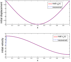
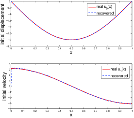
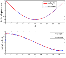
Let $T_{1}=2,T_{2}=2.5$. Then the damping coefficient $q$ can be recovered from (3.13), and the initial values $u_{0}(x)$ and $u_{1}(x)$ can be reconstructed from (3.14). Table 1 lists the numerical results for the damping coefficients (the second column in Table 1) and Figure 1(a)-1(c) for the initial values in various cases of noise levels. In Table 1, the absolute errors of the real damping coefficient and the recovered ones, and the $L^{2}$-norm of the differences between the exact initial values and the reconstructed ones are also shown.

It is worth pointing out that in reconstruction of the initial values from (3.14), the infinite series is approximated by a finite one once again, that is, $\{n\in\mathbb{Z}\}$ is replaced by $\left\{n\in\mathbb{Z}\;|\;|n|\leq 1000\right\}$, which accounts for the zero value of the reconstructed initial velocity at the left end. This is also the reason that the errors of the initial velocity (the last column in Table 1) are relatively large even if there is no random noise in the measured data.

Table 1: Absolute errors with different noise levels

Noise Level	Recovered $q$	Errors for $q$	Errors for $u_{0}(x)$	Errors for $u_{1}(x)$
0	-3.0000	9.3259E-15	1.1744E-08	2.2215E-01
1%	-2.9994	6.2498E-04	1.1618E-03	2.2748E-01
3%	-2.9979	2.0904E-03	3.5604E-03	2.6662E-01

(a) without random noise

(b) with 1% random error

(c) with 3% random error

Figure 1: The initial values: initial displacement (upper) and initial velocity (lower)

Example 3.2.

The observation with general bounded disturbance when system (1.1) is anti-stable.

The anti-damping coefficient and initial values are chosen as

$$q=3,\quad u_{0}(x)=3\sin\pi x,\quad u_{1}(x)=\pi\cos\pi x.$$ (3.19)

and the observation is corrupted by the bounded disturbance:

$$d(t)=2\sin\displaystyle\frac{1}{1+t}+3\cos 10t.$$ (3.20)

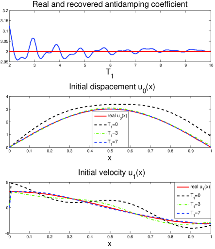
The relevant parameters in Corollary 3.2 are chosen to be $T_{2}=T_{1}+3$, and let $T_{1}$ be different values increasing from $2$ to $10$. The corresponding anti-damping coefficients $q_{T_{1}}$ recovered from (3.16) are depicted in Figure 2. It is seen that $q_{T_{1}}$ converges to the real value $q=3$ as $T_{1}$ increases. Setting $T_{1}=0,\;3,\;7$ in (3.17) and reconstructing the initial values produce results in Figure 2 from which we can see that the reconstructed initial values become closer to the real ones as $T_{1}$ increases.

Figure 2: anti-damping coefficient $q$ and initial values $u_{0},\;u_{1}$

4 Application to Schrödinger equation

In this section, we consider a quantum system described by the following Schrödinger equation:

$$\left\{\begin{array}[]{ll}u_{t}=-iu_{xx}+qu,&0<x<1,\;t>0,\\ u_{x}(0,t)=0,\;\;u(1,t)=0,&t\geq 0,\\ y(t)=u(0,t)+d(t),&t\geq 0,\\ u(x,0)=u_{0}(x),&0\leq x\leq 1.\end{array}\right.$$ (4.1)

where $u(x,t)$ is the complex-valued state, $i$ is the imaginary unit, and the potential $q>0$ and $u_{0}(x)$ are the unknown anti-damping coefficient and initial value, respectively.

Let ${\cal H}=L^{2}(0,1)$ be equipped with the usual inner product $\langle\cdot,\cdot\rangle$ and the inner product induced norm $\|\cdot\|.$ Introduce the operator ${\cal A}$ defined by

$$\left\{\begin{array}[]{l}{\cal A}\phi=-i\phi^{\prime\prime}+q\phi,\\ D({\cal A})=\left\{\phi\in H^{2}(0,1)\;|\;\phi^{\prime}(0)=\phi(1)=0\right\}.\end{array}\right.$$ (4.2)

A straightforward verification shows that such defined ${\cal A}$ generates a $C_{0}$-semigroup on ${\cal H}$.

Lemma 4.1.

[17] Let ${\cal A}$ be defined by (4.2). Then the spectrum of ${\cal A}$ consists of all isolated eigenvalues given by

$$\lambda_{n}=q+i\left(n-\displaystyle\frac{1}{2}\right)^{2}\pi^{2},\quad n\in{\mathbb{N}},$$ (4.3)

and the corresponding eigenfunctions $\phi_{n}(x)$ are given by

$$\phi_{n}(x)=\sqrt{2}\cos\left(n-\displaystyle\frac{1}{2}\right)\pi x,\quad n\in{\mathbb{N}}.$$ (4.4)

In addition, $\{\phi_{n}(x)\}_{n\in{\mathbb{N}}}$ forms an orthonormal basis for ${\cal H}$.

System (4.1) can be rewritten as the following evolutionary equation in ${\cal H}$:

$$\frac{dX(t)}{dt}={\cal A}X(t),\;t>0,\quad X(0)=u_{0},$$ (4.5)

and the solution of (4.5) is given by

$$X(t)=\sum_{n\in{\mathbb{N}}}e^{\lambda_{n}t}\langle X(0),\phi_{n}\rangle\phi_{n}.$$ (4.6)

Thus

$$y(t)=\sqrt{2}\sum_{n\in{\mathbb{N}}}e^{\lambda_{n}t}\langle u_{0},\phi_{n}\rangle+d(t).$$ (4.7)

The relevant function and parameters in Theorems 2.1-2.2 for system (4.1) are

$$f(q)=q,\;\mu_{n}=\left(n-\displaystyle\frac{1}{2}\right)^{2}\pi^{2},\;L=\displaystyle\frac{8}{\pi},\;\kappa_{n}=\sqrt{2}.$$

Parallel to Section 3, we have two corollaries corresponding to the exact observation and observation with general bounded disturbance, respectively, for system (4.1). Here we only list the latter one and the former is omitted.

Corollary 4.1.

Suppose that $q\in Q=(0,+\infty)$ in system (4.1) and the disturbance is bounded, i.e. $|d(t)|\leq M$ for some $M>0$ and all $t\geq 0$. Then for any $T_{2}-\frac{8}{\pi}>T_{1}>\frac{8}{\pi}$,

$$\lim_{T_{1}\rightarrow+\infty}q_{T_{1}}=q,\quad\lim_{T_{1}\rightarrow+\infty}\|\hat{u}_{0T_{1}}-u_{0}\|=0,$$ (4.8)

where

$$q_{T_{1}}=\displaystyle\frac{\pi}{8}\ln\displaystyle\frac{\|y\|_{L^{2}(T_{1},T_{2})}}{\|y\|_{L^{2}(T_{1}-\frac{8}{\pi},T_{2}-\frac{8}{\pi})}},\;\frac{8}{\pi}<T_{1}<T_{2}-\frac{8}{\pi},$$ (4.9)

and

$$\hat{u}_{0T_{1}}(x)=\displaystyle\frac{\pi}{8}\sum_{n\in\mathbb{Z}}\left(\int_{T_{1}}^{T_{1}+\frac{8}{\pi}}y(t)e^{-\lambda_{n}t}dt\right)\cos\left(n-\displaystyle\frac{1}{2}\right)\pi x.$$ (4.10)

We also give a numerical simulation to test the algorithm proposed in Corollary 4.1 for system (4.1), where the anti-damping coefficient $q$ and initial value $u_{0}(x)$ are chosen as

$$q=0.7,\quad u_{0}(x)=\sin\pi x+i\cos\pi x,$$ (4.11)

and the observation is corrupted by the disturbance

$$d(t)=2\sin\displaystyle\frac{t}{10+t}+3i\cos 20t.$$ (4.12)

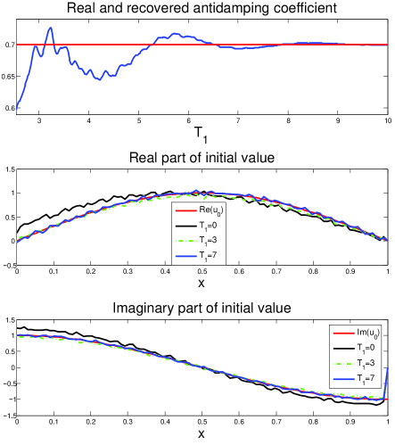
The observation can be obtained from (4.7) by a finite series approximation, that is, $\{n\in{\mathbb{N}}\}$ is replaced by $\left\{n\in{\mathbb{N}}\;|\;n\leq 5000\right\}$. The relevant parameters in Corollary 4.1 are chosen to be $T_{2}=T_{1}+1$, and $T_{1}$ increasing from $2.55$ to $10$. The corresponding anti-damping coefficients $q_{T_{1}}$ recovered from (4.9) are shown in Figure 3. It is obvious that $q_{T_{1}}$ is convergent to the real value $q=0.7$ as $T_{1}$ increases. Setting $T_{1}=0,\;3,\;7$, respectively, in (4.10), the reconstructed initial values are shown in Figure 3 from which it is seen that the errors between the reconstructed initial values and the real ones become smaller as $T_{1}$ increases.

Figure 3: coefficient (upper), real part (middle) and imaginary part (lower) of initial value $u_{0}(x)$

5 Application to coupled strings equation

In this section, we consider the following two connected anti-stable strings with joint anti-damping described by

$$\left\{\begin{array}[]{l}u_{tt}(x,t)=u_{xx}(x,t),x\in(0,\frac{1}{2})\cup(\frac{1}{2},1),\;t>0,\\ u\left(\frac{1}{2}^{-},t\right)=u\left(\frac{1}{2}^{+},t\right),\;t\geq 0,\\ u_{x}\left(\frac{1}{2}^{-},t\right)-u_{x}\left(\frac{1}{2}^{+},t\right)=qu_{t}(1,t),\;t\geq 0,\\ u(0,t)=u_{x}(1,t)=0,\;t\geq 0,\\ u(x,0)=u_{0}(x),u_{t}(x,0)=u_{1}(x),\;0\leq x\leq 1,\\ y(t)=u_{x}(0,t)+d(t),\;t\geq 0,\end{array}\right.$$ (5.1)

where $q>0,q\neq 2$ is the unknown anti-damping constant. System (5.1) models two connected strings with joint vertical force anti-damping, see [10, 11, 22] for more details.

Let ${\cal H}=H_{E}^{1}(0,1)\times L^{2}(0,1)$ be equipped with the inner product $\langle\cdot,\cdot\rangle$ and its induced norm

$$\|(u,v)\|^{2}=\displaystyle\int_{0}^{1}\left[|u^{\prime}(x)|^{2}+|v(x)|^{2}\right]dx,$$

where $H_{E}^{1}(0,1)=\left\{u|\;u\in H^{1}(0,1),u(0)=0\right\}$. Then system (5.1) can be rewritten as an evolutionary equation in ${\cal H}$ as follows:

$$\frac{d}{dt}X(t)={\cal A}X(t),$$ (5.2)

where $X(t)=(u(\cdot,t),u_{t}(\cdot,t))\in{\cal H}$ and ${\cal A}$ is defined by

$${\cal A}(u,v)=(v(x),u^{\prime\prime}(x)),$$ (5.3)

with the domain

$$\begin{array}[]{l}D({\cal A})=\left\{(u,v)\in H^{1}(0,1)\times H_{E}^{1}(0,1)\Bigg{|}\begin{array}[]{l}u(0)=u^{\prime}(1)=0,\;u|_{[0,\frac{1}{2}]}\in H^{2}(0,\frac{1}{2}),\\ u|_{[\frac{1}{2},1]}\in H^{2}(\frac{1}{2},1),\;u^{\prime}(\frac{1}{2}^{-})-u^{\prime}(\frac{1}{2}^{+})=qv(\frac{1}{2}),\end{array}\right\},\end{array}$$ (5.4)

where $u|_{[a,b]}$ denotes the function $u(x)$ confined to $[a,b]$.

We assume without loss of generality that the prior parameter set for $q$ is $Q=(2,+\infty)$ since the case for $Q=(0,2)$ is very similar.

Lemma 5.1.

[22] Let ${\cal A}$ be defined by (5.3)-(5.4) and $q\in Q=(2,+\infty)$. Then ${\cal A}^{-1}$ is compact on ${\cal H}$ and the eigenvalues of ${\cal A}$ are algebraically simple and separated, given by

$$\lambda_{n}=\displaystyle\frac{1}{2}\ln\displaystyle\frac{q+2}{q-2}+in\pi,\;n\in\mathbb{Z}.$$ (5.5)

The corresponding eigenfunctions $\Phi_{n}(x)$ are given by

$$\Phi_{n}(x)=(\phi_{n}(x),\lambda_{n}\phi_{n}(x)),\;\forall\;n\in\mathbb{Z},$$ (5.6)

where

$$\phi_{n}(x)=\left\{\begin{array}[]{ll}\displaystyle\frac{\sqrt{2}}{\lambda_{n}}\cosh\displaystyle\frac{\lambda_{n}}{2}\sinh\lambda_{n}x,&0<x<\displaystyle\frac{1}{2},\cr\vskip 5.69054pt\cr\displaystyle\displaystyle\frac{\sqrt{2}}{\lambda_{n}}\sinh\displaystyle\frac{\lambda_{n}}{2}\cosh\lambda_{n}(1-x),&\displaystyle\frac{1}{2}<x<1.\end{array}\right.$$

and $\{\Phi_{n}(x)\}_{n\in\mathbb{Z}}$ forms a Riesz basis for ${\cal H}$. In addition, ${\cal A}$ generates a $C_{0}$-semigroup on ${\cal H}$.

Lemma 5.2.

[22] Let ${\cal A}$ be defined by (5.3)-(5.4) and $q\in Q=(2,+\infty)$. Then the adjoint operator ${\cal A}^{\ast}$ of ${\cal A}$ is given by

$${\cal A}^{\ast}(u,v)=-(v,u^{\prime\prime}),$$ (5.7)

with the domain

$$\begin{array}[]{l}D({\cal A}^{\ast})=\left\{(u,v)\in H^{1}(0,1)\times H_{E}^{1}(0,1)\Bigg{|}\begin{array}[]{l}u(0)=u^{\prime}(1)=0,\;u|_{[0,\frac{1}{2}]}\in H^{2}(0,\frac{1}{2}),\\ u|_{[\frac{1}{2},1]}\in H^{2}(\frac{1}{2},1),\;u^{\prime}(\frac{1}{2}^{-})-u^{\prime}(\frac{1}{2}^{+})=-qv(\frac{1}{2})\end{array}\right\},\end{array}$$

and $\sigma({\cal A}^{\ast})=\sigma({\cal A})$. The eigenfunctions $\Psi_{n}(x)$ of ${\cal A}^{\ast}$ corresponding to $\overline{\lambda}_{n}$ are given by

$$\Psi_{n}(x)=\left(\overline{\phi}_{n}(x),-\overline{\lambda}_{n}\overline{\phi}_{n}(x)\right),\quad\forall\;n\in\mathbb{Z}.$$ (5.8)

A direct calculation shows that $\{\Psi_{n}(x)\}$ is biorthogonal to $\{\Phi_{n}(x)\}$. Hence, the solution of (5.2) can be expressed as

$$X(t)=\sum_{n\in\mathbb{Z}}e^{\lambda_{n}t}\langle X(0),\Psi_{n}\rangle\Phi_{n}.$$ (5.9)

Define the observation operator $\mathcal{C}$ from ${\cal H}$ to ${\mathbb{C}}$ to be

$$\mathcal{C}(f,g)=f^{\prime}(0),\quad(f,g)\in D({\cal A}).$$ (5.10)

Then

$$y(t)=\sum_{n\in\mathbb{Z}}e^{\lambda_{n}t}\langle X(0),\Psi_{n}\rangle\mathcal{C}\Phi_{n}+d(t).$$ (5.11)

The succeeding Corollary 5.1 is a direct consequence of Theorem 2.2 by noticing that for system (5.1), the relevant function and parameters now are

$$f(q)=\displaystyle\frac{1}{2}\ln\displaystyle\frac{q+2}{q-2},\;\mu_{n}=n\pi,\;L=2,\;\kappa_{n}=\sqrt{2}\cosh\displaystyle\frac{\lambda_{n}}{2},$$

and a simple calculation shows that

$$\frac{\sqrt{2}}{2}\left[\left(\displaystyle\frac{q+2}{q-2}\right)^{\frac{1}{4}}-\left(\displaystyle\frac{q-2}{q+2}\right)^{\frac{1}{4}}\right]\leq|\kappa_{n}|\leq\displaystyle\frac{\sqrt{2}}{2}\left[\left(\displaystyle\frac{q+2}{q-2}\right)^{\frac{1}{4}}+\left(\displaystyle\frac{q-2}{q+2}\right)^{\frac{1}{4}}\right],\;\;\forall\;n\in\mathbb{Z}.$$

The corollaries corresponding to Theorem 2.1 are omitted here.

Corollary 5.1.

Suppose that $q\in Q=(2,+\infty)$ in system (5.1) and the disturbance is bounded, i.e. $|d(t)|\leq M$ for some $M>0$ and all $t\geq 0$. Then for any $T_{2}-2>T_{1}\geq 2$,

$$\lim_{T_{1}\rightarrow+\infty}q_{T_{1}}=q,\;\lim_{T_{1}\rightarrow+\infty}\|(\hat{u}_{0T_{1}},\hat{u}_{1T_{1}})-(u_{0},u_{1})\|=0,$$

where

$$q_{T_{1}}=\displaystyle\frac{2\left(\|y\|_{L^{2}(T_{1},T_{2})}+\|y\|_{L^{2}(T_{1}-2,T_{2}-2)}\right)}{\|y\|_{L^{2}(T_{1},T_{2})}-\|y\|_{L^{2}(T_{1}-2,T_{2}-2)}},$$ (5.12)

and

$$\begin{array}[]{l}\hat{u}_{0T_{1}}(x)=\left\{\begin{array}[]{ll}\displaystyle\displaystyle\frac{1}{2}\sum_{n\in\mathbb{Z}}\left(\int_{T_{1}}^{T_{1}+2}y(t)e^{-\lambda_{n}t}dt\right)\displaystyle\frac{\sinh\lambda_{n}x}{\lambda_{n}},&0<x<\displaystyle\frac{1}{2},\\ \displaystyle\displaystyle\frac{1}{2}\sum_{n\in\mathbb{Z}}\left(\int_{T_{1}}^{T_{1}+2}y(t)e^{-\lambda_{n}t}dt\right)\tanh\displaystyle\frac{\lambda_{n}}{2}\displaystyle\frac{\cosh\lambda_{n}(1-x)}{\lambda_{n}},&\displaystyle\frac{1}{2}<x<1.\end{array}\right.\cr\vskip 5.69054pt\cr\displaystyle\hat{u}_{1T_{1}}(x)=\left\{\begin{array}[]{ll}\displaystyle\displaystyle\frac{1}{2}\sum_{n\in\mathbb{Z}}\left(\int_{T_{1}}^{T_{1}+2}y(t)e^{-\lambda_{n}t}dt\right)\sinh\lambda_{n}x,&0<x<\displaystyle\frac{1}{2},\\ \displaystyle\displaystyle\frac{1}{2}\sum_{n\in\mathbb{Z}}\left(\int_{T_{1}}^{T_{1}+2}y(t)e^{-\lambda_{n}t}dt\right)\tanh\displaystyle\frac{\lambda_{n}}{2}\cosh\lambda_{n}(1-x),&\displaystyle\frac{1}{2}<x<1.\end{array}\right.\end{array}$$ (5.13)

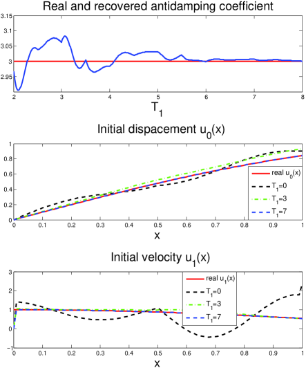
As before, we present some numerical simulations for system (5.1) to showcase the effectiveness of the algorithm proposed in Corollary 5.1. The anti-damping coefficient $q$ and initial values $u_{0}(x)$ and $u_{1}(x)$ are chosen to be

$$q=3,\quad u_{0}(x)=\sin x,\quad u_{1}(x)=\cos x,$$ (5.14)

and the observation is corrupted by the disturbance

$$d(t)=\sin\displaystyle\frac{t^{2}}{10+t}+\cos 10t.$$ (5.15)

The observation is obtained from (5.11) by a finite series approximation, that is, $\{n\in{\mathbb{N}}\}$ is replaced by $\left\{n\in{\mathbb{N}}|\;|n|\leq 5000\right\}$. The relevant parameters in Corollary 5.1 are chosen to be $T_{2}=T_{1}+1$, and $T_{1}$ increases from $2$ to $8$. The corresponding anti-damping coefficients $q_{T_{1}}$ recovered from (5.12) are plotted in Figure 4. It can be seen that $q_{T_{1}}$ converges to the real value $q=3$ as $T_{1}$ increases. Let $T_{1}=0,\;3,\;7$ in (5.13), and the reconstructed initial values are shown in Figure 4, from which it is seen that the reconstructed initial values become closer to the real ones as $T_{1}$ increases.

Figure 4: anti-damping coefficient $q$ (upper), initial values $u_{0}$ (middle) and $u_{1}$ (lower)

6 Concluding remarks

In this paper, we propose an algorithm to reconstruct simultaneously an anti-damping coefficient and an initial value for some anti-stable PDEs. When the measured output is exact, the recovered values are exact whereas if the measured output suffers from bounded unknown disturbance, the approximated values of the anti-damping coefficient and initial value can also be obtained. Some numerical examples are carried out to validate the effectiveness of the algorithm. It is very promising to apply the algorithm presented here to stabilization of anti-stable systems with an unknown anti-damping coefficient.

References

- [1] S.A. Avdonin and S.A. Ivanov, Families of Exponentials: The Method of Moments in Controllability Problems for Distributed Parameter Systems, Cambridge University Press, 1995.
- [2] S.A. Avdonin and W. Moran, Ingham-type inequalities and Riesz bases of divided differences, Int. J. Appl. Math. Comput. Sci., 11(2001), 803–820.
- [3] S.A. Avdonin and S.A. Ivanov, Riesz bases of exponentials and divided differences, St. Petersburg Math. J., 13(2002), 339–351.
- [4] H.T. Banks and I.G. Rosen, Computational methods for the identification of spatially varying stiffness and damping in beams, Control Theory Adv. Tech., 3(1987), 1–32.
- [5] H.T. Banks and K. Ito, A unified framework for approximation in inverse problems for distributed parameter systems, Control Theory Adv. Tech., 4(1988), 73–90.
- [6] H.T. Banks and K. Kunisch, Estimation Techniques for Distributed Parameter System, Birkhäuser, Boston, 1989.
- [7] D. Bresch-Pietri and M. Krstic, Output-feedback adaptive control of a wave PDE with boundary anti-damping, Automatica, 50(2014), 1407–1415.
- [8] B.Z. Guo and Y.H. Luo, Controllability and stability of a second-order hyperbolic system with collocated sensor/actuator, Systems Control Lett., 46(2002), 45–65.
- [9] B.Z. Guo and Y.H. Luo, Riesz basis property of a second-order hyperbolic system with collocated scalar input-output, IEEE Trans. Autom. Control, 47(2002), 693–698.
- [10] B.Z. Guo and W.D. Zhu, On the energy decay of two coupled strings through a joint damper, J. Sound Vib., 203(1997), 447–455.
- [11] B.Z. Guo and F.F. Jin, Arbitrary decay rate for two connected strings with joint anti-damping by boundary output feedback, Automatica, 46(2010), 1203–1209.
- [12] B.Z. Guo and F.F. Jin, Sliding mode and active disturbance rejection control to stabilization of one-dimensional anti-stable wave equations subject to disturbance in boundary input, IEEE Trans. Autom. Control, 58(2013), 1269–1274.
- [13] B.Z. Guo and F.F. Jin, Output feedback stabilization for one-dimensional wave equation subject to boundary disturbance, IEEE Trans. Autom. Control, 60(2015), 824–830.
- [14] A.E. Ingham, Some trigonometrical inequalities with applications in the theory of series, Math. Z., 41(1936), 367–379.
- [15] V. Komornik and P. Loreti, Fourier Series in Control Theory, Springer-Verlag, New York, 2005.
- [16] M. Krstic, Adaptive control of an anti-stable wave PDE, Dyn. Contin. Discrete Impuls. Syst. Ser. A. Math. Anal., 17(2010), 853–882.
- [17] M. Krstic, B.Z. Guo, and A. Smyshlyaev, Boundary controllers and observers for the linearized Schrödinger equation, SIAM J. Control Optim., 49(2011), 1479–1497.
- [18] K. Ramdani, M. Tucsnak, and G. Weiss, Recovering the initial state of an infinite-dimensional system using observers, Automatica, 46(2010), 1616–1625.
- [19] A. Smyshlyaev and M. Krstic, Boundary control of an anti-stable wave equation with anti-damping on the uncontrolled boundary, Systems Control Lett., 58(2009), 617–623.
- [20] G. Weiss, Admissible observation operators for linear semigroups, Israel J. Math., 65(1989), 17-43.
- [21] G.Q. Xu, State reconstruction of a distributed parameter system with exact observability, J. Math. Anal. Appl., 409(2014), 168–179.
- [22] G.Q. Xu and B.Z. Guo, Riesz basis property of evolution equations in Hilbert spaces and application to a coupled string equation, SIAM J. Control Optim., 42(2003), 966–984.
- [23] R. M. Young, An Introduction to Nonharmonic Fourier Series, Academic Press, New York, 1980.