Probing the Geometry of Data with Diffusion Fréchet Functions

Abstract

Many complex ecosystems, such as those formed by multiple microbial taxa, involve intricate interactions amongst various sub-communities. The most basic relationships are frequently modeled as co-occurrence networks in which the nodes represent the various players in the community and the weighted edges encode levels of interaction. In this setting, the composition of a community may be viewed as a probability distribution on the nodes of the network. This paper develops methods for modeling the organization of such data, as well as their Euclidean counterparts, across spatial scales. Using the notion of diffusion distance, we introduce diffusion Fréchet functions and diffusion Fréchet vectors associated with probability distributions on Euclidean space and the vertex set of a weighted network, respectively. We prove that these functional statistics are stable with respect to the Wasserstein distance between probability measures, thus yielding robust descriptors of their shapes.

We apply the methodology to investigate bacterial communities in the human gut, seeking to characterize divergence from intestinal homeostasis in patients with Clostridium difficile infection (CDI) and the effects of fecal microbiota transplantation, a treatment used in CDI patients that has proven to be significantly more effective than traditional treatment with antibiotics. The proposed method proves useful in deriving a biomarker that might help elucidate the mechanisms that drive these processes.

1 Introduction

The state of a complex ecosystem is frequently described by a probability distribution on the nodes of a weighted network. For example, a microbial community may be modeled on a network in which each node represents a taxon and the main interactions between pairs of taxa are represented by weighted edges, the weights reflecting the levels of interaction. In this formulation, bacterial relative abundance in a sample may be viewed as a probability distribution $\xi$ on the vertex set $V$ of the network. Thus, $\xi$ describes the composition of the community whereas the underlying network encodes the expected interactions amongst the various taxa. Identifying sub-communities and their organization at different scales from such data, quantifying variation across samples, and integrating information across scales are core problems. Similar questions arise in other contexts such as probability measures defined on Euclidean spaces or other metric spaces. To address these problems, we develop methods that (i) capture the geometry of data and probability measures across a continuum of spatial scales and (ii) integrate information obtained at all scales. In this paper, we focus on the Euclidean and network cases. We analyze distributions with the aid of a 1-parameter family of diffusion metrics $d_{t}$, $t>0$, where $t$ is treated as the scale parameter [1]. For (Borel) probability measures $\alpha$ on $\mathbb{R}^{d}$, our approach is based on a functional statistic $V_{\alpha,t}\colon\mathbb{R}^{d}\to\mathbb{R}$ derived from $d_{t}$ and termed the diffusion Fréchet function of $\alpha$ at scale $t$. Similarly, we define diffusion Fréchet vectors $F_{\xi,t}$ associated with a distribution $\xi$ on the vertex set of a network.

The (classical) Fréchet function of a random variable $y\in\mathbb{R}^{d}$ distributed according to a probability measure $\alpha$ with finite second moment is defined as

$$V_{\alpha}(x)=\mathbb{E}_{\alpha}\!\left[\|y-x\|^{2}\right]=\int_{\mathbb{R}^{d}}\|y-x\|^{2}\,d\alpha(y)\,.$$ (1)

The Fréchet function quantifies the scatter of $y$ about the point $x$ and depends only on $\alpha$. It is well-known that the mean (or expected value) of $y$ is the unique minimizer of $V_{\alpha}$. For complex distributions, aiming at more effective descriptors, we introduce diffusion Fréchet functions and show that they encode a wealth of information about the shape of $\alpha$. At scale $t>0$, we define the diffusion Fréchet function $V_{\alpha,t}\colon\mathbb{R}^{d}\to\mathbb{R}$ by

$$V_{\alpha,t}(x)=\mathbb{E}_{\alpha}\!\left[d_{t}^{2}(y,x)\right]=\int_{\mathbb{R}^{d}}d_{t}^{2}(y,x)\,d\alpha(y)\,.$$ (2)

This definition simply replaces the Euclidean distance in (1) with the diffusion distance $d_{t}$. $V_{\alpha,t}(x)$ may be viewed as a localized second moment of $\alpha$ about $x$. In the network setting, Fréchet vectors are defined in a similar manner through the diffusion kernel associated with the graph Laplacian. Unlike $V_{\alpha}$ that is a quadratic function, diffusion Fréchet functions and vectors typically exhibit rich profiles that reflect the shape of the distribution at different scales. We illustrate this point with simulated data and exploit it in an application to the analysis of microbiome data associated with Clostridium difficile infection (CDI). On the theoretical front, we prove stability theorems for diffusion Fréchet functions and vectors with respect to the Wasserstein distance between probability measures [2]. The stability results ensure that both $V_{\alpha,t}$ and $F_{\xi,t}$ yield robust descriptors, useful for data analysis.

As explained in detail below, $V_{\alpha,t}$ is closely related to the solution of the heat equation $\partial_{t}u=\Delta u$ with initial condition $\alpha$. In particular, if $p_{1},\ldots,p_{n}\in\mathbb{R}^{d}$ are data points sampled from $\alpha$, then the diffusion Fréchet functions for the empirical measure $\alpha_{n}=\frac{1}{n}\sum_{i=1}^{n}\delta_{p_{i}}$ give a reinterpretation of Gaussian density estimators derived from the data as localized second moments of $\alpha_{n}$. An interesting consequence of this fact is that, for the Gaussian kernel, the scale-space model for data on the real line investigated in [3] may be recast as a 1-parameter family of diffusion Fréchet functions.

The rest of the paper is organized as follows. Section 2 reviews the concept of diffusion distance in the Euclidean and network settings. We define multiscale diffusion Fréchet functions in Section 3 and prove that they are stable with respect to the Wasserstein distance between probability measures defined in Euclidean spaces. The network counterpart is developed in Section 4. In Section 5 we describe and analyze microbiome data associated with C. difficile infection. We conclude with a summary and some discussion in Section 6.

2 Diffusion Distances

Our multiscale approach to probability measures uses a formulation derived from the notion of diffusion distance [1]. In this section, we review diffusion distances associated with the heat kernel on $\mathbb{R}^{d}$, followed by a discrete analogue for weighted networks.

For $t>0$, let $G_{t}\colon\mathbb{R}^{d}\times\mathbb{R}^{d}\to\mathbb{R}$ be the diffusion (heat) kernel

$$G_{t}(x,y)=\frac{1}{C_{d}(t)}\exp\left(-\frac{\|y-x\|^{2}}{4t}\right)\,,$$ (3)

where $C_{d}(t)=(4\pi t)^{d/2}$. If an initial distribution of mass on $\mathbb{R}^{d}$ is described by a Borel probability measure $\alpha$ and its time evolution is governed by the heat equation $\partial_{t}u=\Delta u$, then the distribution at time $t$ has a smooth density function $\alpha_{t}(y)=u(y,t)$ given by the convolution

$$u(y,t)=\int_{\mathbb{R}^{d}}G_{t}(x,y)\,d\alpha(x)\,.$$ (4)

For an initial point mass located at $x\in\mathbb{R}$, $\alpha$ is Dirac’s delta $\delta_{x}$ and $u(y,t)=G_{t}(x,y)$.

The diffusion map $\Psi_{t}\colon\mathbb{R}^{d}\to\mathbb{L}_{2}(\mathbb{R}^{d})$, given by $\Psi_{t}(x)=G_{t}(x,\cdot)$, embeds $\mathbb{R}^{d}$ into $\mathbb{L}_{2}(\mathbb{R}^{d})$. The diffusion distance $d_{t}$ on $\mathbb{R}^{d}$ is defined as

$$d_{t}(x_{1},x_{2})=\|\Psi_{t}(x_{1})-\Psi_{2}(x_{2})\|_{2}\,,$$ (5)

the metric that $\mathbb{R}^{d}$ inherits from $\mathbb{L}_{2}(\mathbb{R}^{d})$ via the embedding $\psi_{t}$. A calculation shows that

$$\begin{split}d^{2}_{t}(x_{1},x_{2})&=\|\Psi_{t}(x_{1})\|^{2}_{2}+\|\Psi_{t}(x_{2})\|^{2}_{2}-2G_{2t}(x_{1},x_{2})\\ &=2\left(\frac{1}{C_{d}(2t)}-G_{2t}(x_{1},x_{2})\right)\,,\end{split}$$ (6)

where we used the fact that $\|\Psi_{t}(x)\|^{2}_{2}=1/C_{d}(2t)$, for every $x\in\mathbb{R}^{d}$. Note that this implies that the metric space $(\mathbb{R}^{d},d_{t})$ has finite diameter.

Diffusion distances on weighted networks may be defined in a similar way by invoking the graph Laplacian and the associated diffusion kernel. Let $v_{1},\ldots,v_{n}$ be the nodes of a weighted network $K$. The weight of the edge between $v_{i}$ and $v_{j}$ is denoted $w_{ij}$, with the convention that $w_{ij}=0$ if there is no edge between the nodes. We let $W$ be the $n\times n$ matrix whose $(i,j)$-entry is $w_{ij}$. The graph Laplacian is the $n\times n$ matrix $\Delta=D-W$, where $D$ is the diagonal matrix with $d_{ii}=\sum_{k=1}^{n}w_{ik}$, the sum of the weights of all edges incident with the node $v_{i}$ (cf. [4]). This definition is based on a finite difference discretization of the Laplacian, except for a sign that makes $\Delta$ a positive semi-definite, symmetric matrix. The diffusion (or heat) kernel at $t>0$ is the matrix $e^{-t\Delta}$.

Let $\xi$ be a probability distribution on the vertex set $V$ of $K$. If $\xi_{i}\geq 0$, $1\leq i\leq n$, is the probability of the vertex $v_{i}$, we write $\xi$ as the vector $\xi=[\xi_{1}\,\ldots\,\xi_{n}]^{T}\in\mathbb{R}^{n}$, where $T$ denotes transposition. Clearly, $\xi_{1}+\ldots+\xi_{n}=1$. Note that $u=e^{-t\Delta}\xi$ solves the heat equation $\partial_{t}u=-\Delta u$ with initial condition $\xi$. (The negative sign is due to the convention made in the definition of $\Delta$.) Mass initially distributed according to $\xi$, whose diffusion is governed by the heat equation, has time $t$ distribution $u_{t}=e^{-t\Delta}\xi$. A point mass at the $i$th vertex is described by the vector $e_{i}\in\mathbb{R}^{n}$, whose $j$th entry is $\delta_{ij}$. Thus, $e^{-t\Delta}e_{i}$ may be viewed as a network analogue of the Gaussian $G_{t}(x,\cdot)$. For $t>0$, the diffusion mapping $\psi_{t}\colon V\to\mathbb{R}^{n}$ is defined by $\psi_{t}(v_{i})=e^{-t\Delta}e_{i}$ and the time $t$ diffusion distance between the vertices $v_{i}$ and $v_{j}$ by

$$d_{t}(i,j)=\|e^{-t\Delta}e_{i}-e^{-t\Delta}e_{j}\|\,,$$ (7)

where $\|\cdot\|$ denotes Euclidean norm. If $0=\lambda_{1}\leq\ldots\leq\lambda_{n}$ are the eigenvalues of $\Delta$ with orthonormal eigenvectors $\phi_{1},\ldots,\phi_{n}$, then

$$d_{t}^{2}(i,j)=\sum_{k=1}^{n}e^{-2\lambda_{k}t}\left(\phi_{k}(i)-\phi_{k}(j)\right)^{2}\,,$$ (8)

where $\phi_{k}(i)$ denotes the $i$th component of $\phi_{k}$ [1].

3 Diffusion Fréchet Functions

The classical Fréchet function $V_{\alpha}$ of a probability measure $\alpha$ on $\mathbb{R}^{d}$ with finite second moment is a useful statistic. However, for complex distributions, such as those with a multimodal profile or more intricate geometry, their Fréchet functions usually fail to provide a good description of their shape. Aiming at more effective descriptors, we introduce diffusion Fréchet functions and show that they encode a wealth of information across a full range of spatial scales. At scale $t>0$, define the diffusion Fréchet function $V_{\alpha,t}\colon\mathbb{R}^{d}\to\mathbb{R}$ by

$$V_{\alpha,t}(x)=\int_{\mathbb{R}^{d}}d_{t}^{2}(y,x)\,d\alpha(y)\,.$$ (9)

Note that $V_{\alpha,t}$ is defined for any Borel probability measure $\alpha$, not just those with finite second moment, because $(\mathbb{R}^{d},d_{t})$ has finite diameter. Moreover, $V_{\alpha,t}$ is uniformly bounded. We also point out that this construction is distinct from the standard kernel trick that pushes $\alpha$ forward to a probability measure $(\psi_{t})_{\ast}(\alpha)$ on $\mathbb{L}_{2}(\mathbb{R}^{d})$, where the usual Fréchet function of $(\psi_{t})_{\ast}(\alpha)$ can be used to define such notions as an extrinsic mean of $\alpha$. $V_{t}$ is an intrinsic statistic and typically a function on $\mathbb{R}^{d}$ with a complex profile, as we shall see in the examples below. From (2) and (6), it follows that

$$\begin{split}V_{\alpha,t/2}(x)=\frac{2}{C_{d}(t)}-2\int_{\mathbb{R}^{d}}G_{t}(x,y)\,d\alpha(y)=\frac{2}{C_{d}(t)}-2\alpha_{t}(x)\,,\end{split}$$ (10)

where $\alpha_{t}(x)=u(x,t)$, the solution of the heat equation $\partial_{t}u=\Delta u$ with initial condition $\alpha$.

If $p_{1},\ldots,p_{n}\in\mathbb{R}^{d}$ are data points sampled from $\alpha$, then the diffusion Fréchet function of the empirical measure $\alpha_{n}=\frac{1}{n}\sum_{i=1}^{n}\delta_{p_{i}}$ is closely related to the Gaussian density estimator $\widehat{\alpha}_{n,t}=\frac{1}{n}\sum_{i=1}^{n}G_{t}(x,p_{i})$ derived from the sample points. Indeed, it follows from (10) that

$$\begin{split}V_{\alpha_{n},t/2}(x)=\frac{2}{C_{d}(t)}-2\int_{\mathbb{R}^{d}}G_{t}(x,y)\,d\alpha_{n}(y)=\frac{2}{C_{d}(t)}-2\widehat{\alpha}_{n,t}(x)\,.\end{split}$$ (11)

Thus, diffusion Fréchet functions provide a new interpretation of Gaussian density estimators, essentially as second moments with respect to diffusion distances. This opens up interesting new perspectives. For example, the classical Fréchet function $V_{\alpha}\colon\mathbb{R}^{d}\to\mathbb{R}$ (see (1)) may be viewed as the trace of the covariance tensor field $\Sigma^{\alpha}\colon\mathbb{R}^{d}\to\mathbb{R}^{d}\otimes\mathbb{R}^{d}$ given by

$$\Sigma_{\alpha}(x)=\mathbb{E}_{\alpha}\!\left[(y-x)\otimes(y-x)\right]=\int_{\mathbb{R}^{d}}(y-x)\otimes(y-x)\,d\alpha(y)\,.$$ (12)

Thus, it is natural to ask: How to define diffusion covariance tensor fields $\Sigma_{\alpha,t}$ that capture the modes of variation of $\alpha$, about each $x\in\mathbb{R}^{d}$ at all scales, bearing a close relationship to $V_{\alpha,t}$? A multiscale approach to data along related lines has been developed in [5, 6].

Example 1.

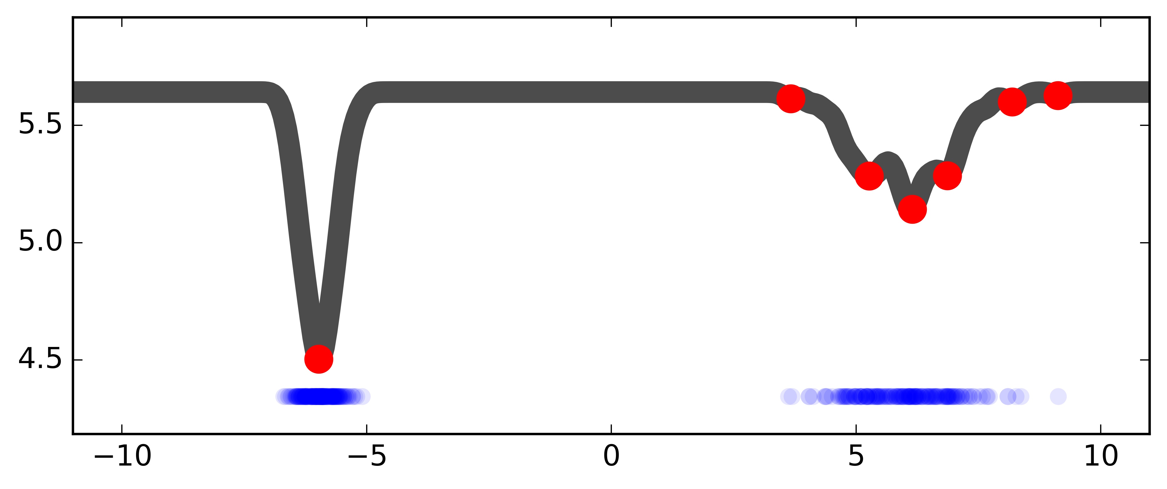
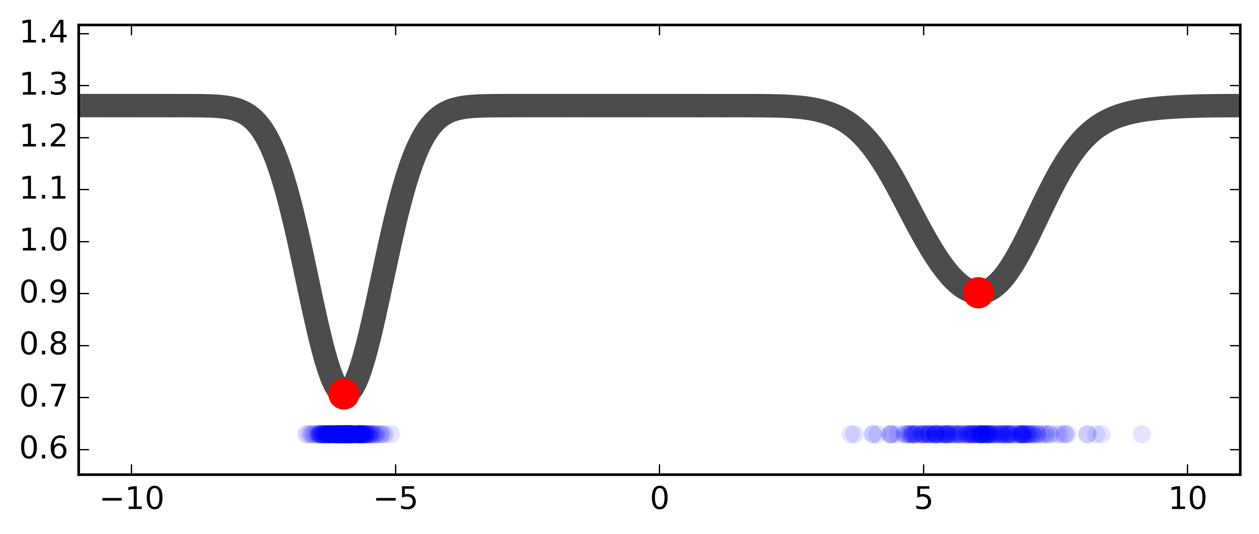
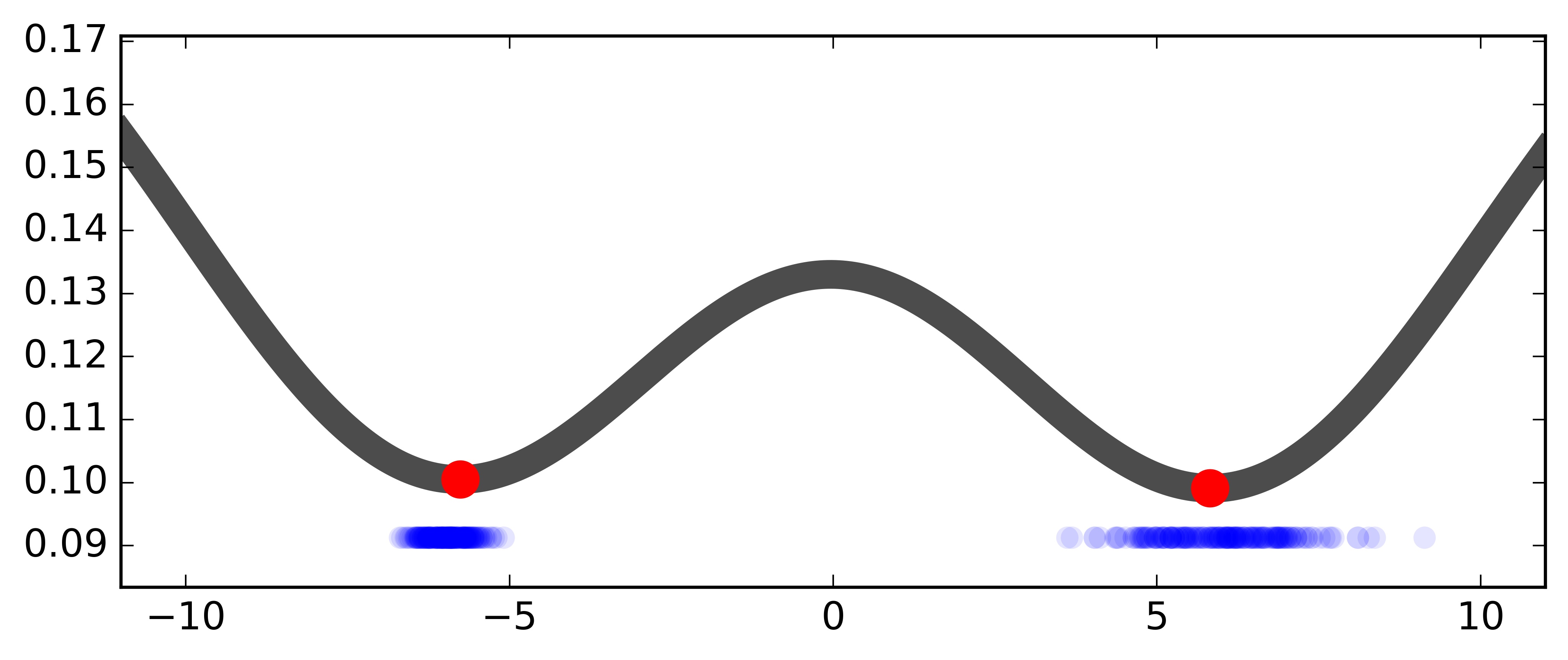
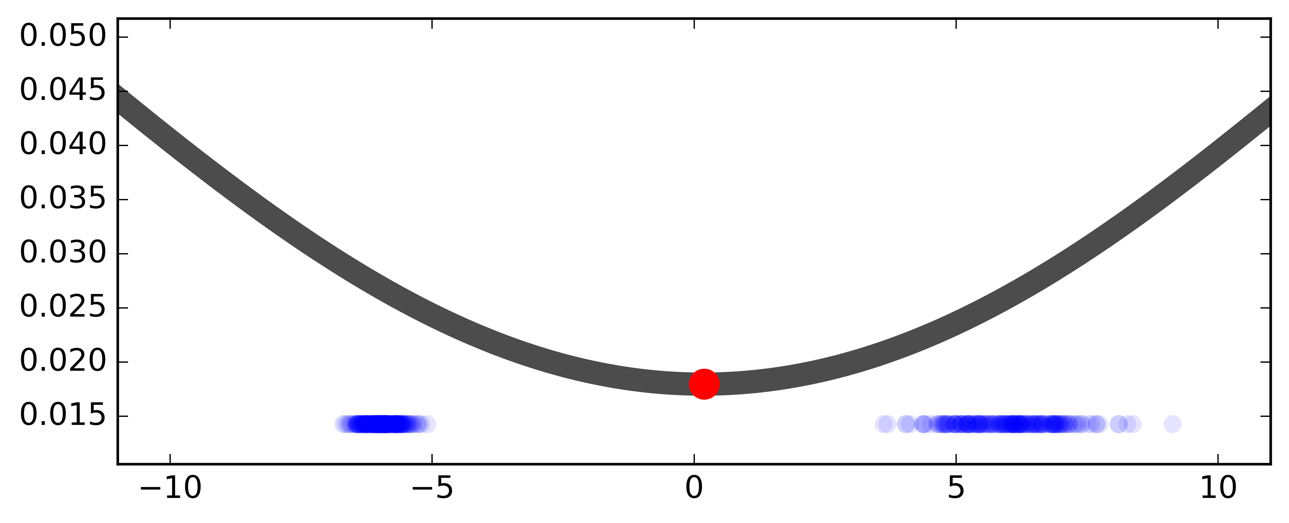
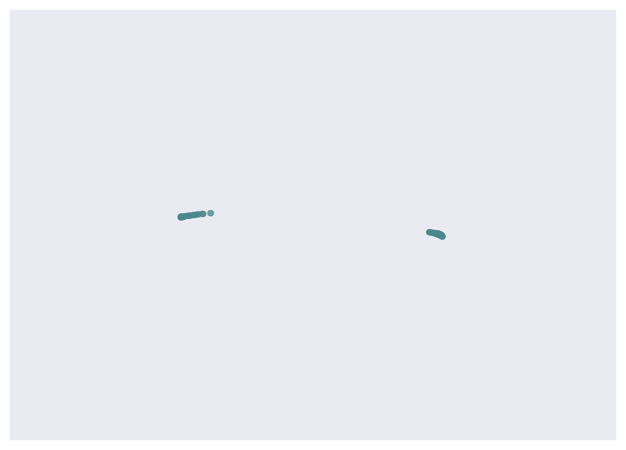
Here we consider the dataset highlighted in blue in Figure 1, comprising $n=400$ points $p_{1},\ldots,p_{n}$ on the real line, grouped into two clusters. The figure shows the evolution of the diffusion Fréchet function for the empirical measure $\alpha_{n}=\sum_{i=1}^{n}\delta_{p_{i}}/n$ for increasing values of the scale parameter.

$t=0.005$	$t=0.1$
$t=4$	$t=20$

Figure 1: Evolution of the diffusion Fréchet function across scales.

At scale $t=0.1$, the Fréchet function has two well defined “valleys”, each corresponding to a data cluster. At smaller scales, $V_{\alpha_{n},t}$ captures finer properties of the organization of the data, whereas at larger scales $V_{\alpha_{n},t}$ essentially views the data as comprising a single cluster. For probability distributions on the real line, the Fréchet function levels off to $1/\sqrt{2\pi t}$, as $|x|\to\infty$. The local minima of $V_{\alpha,t}$ provide a generalization of the mean of the distribution and a summary of the organization of the data into sub-communities across multiple scales. Elucidating such organization in data in an easily interpretable manner is one of our principal aims.

Example 2.

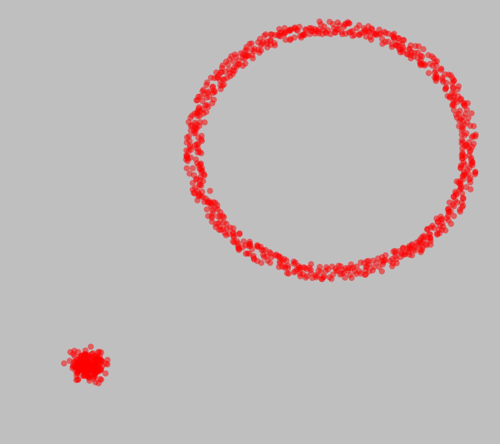
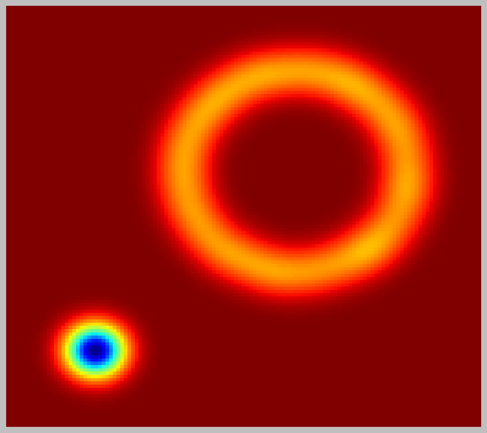
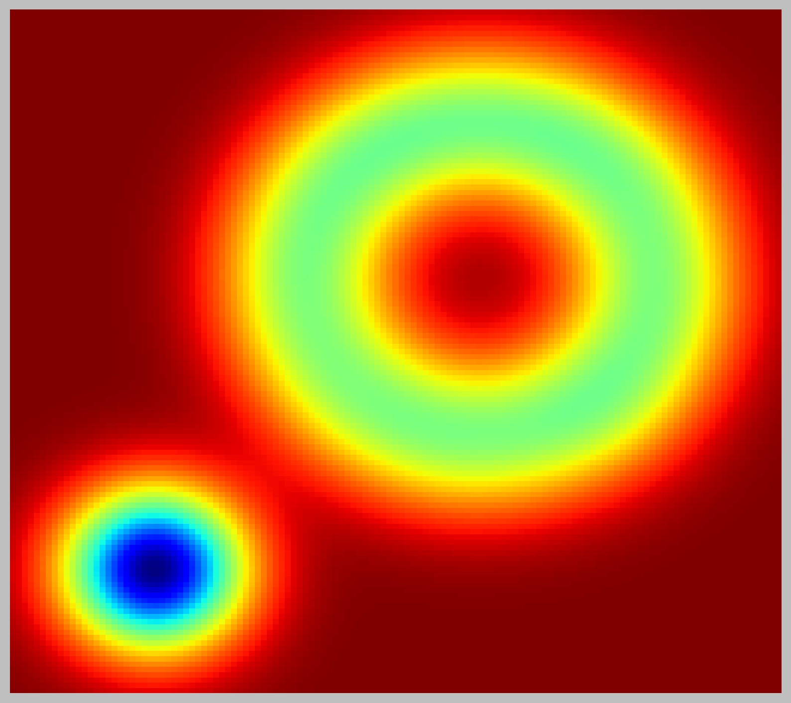
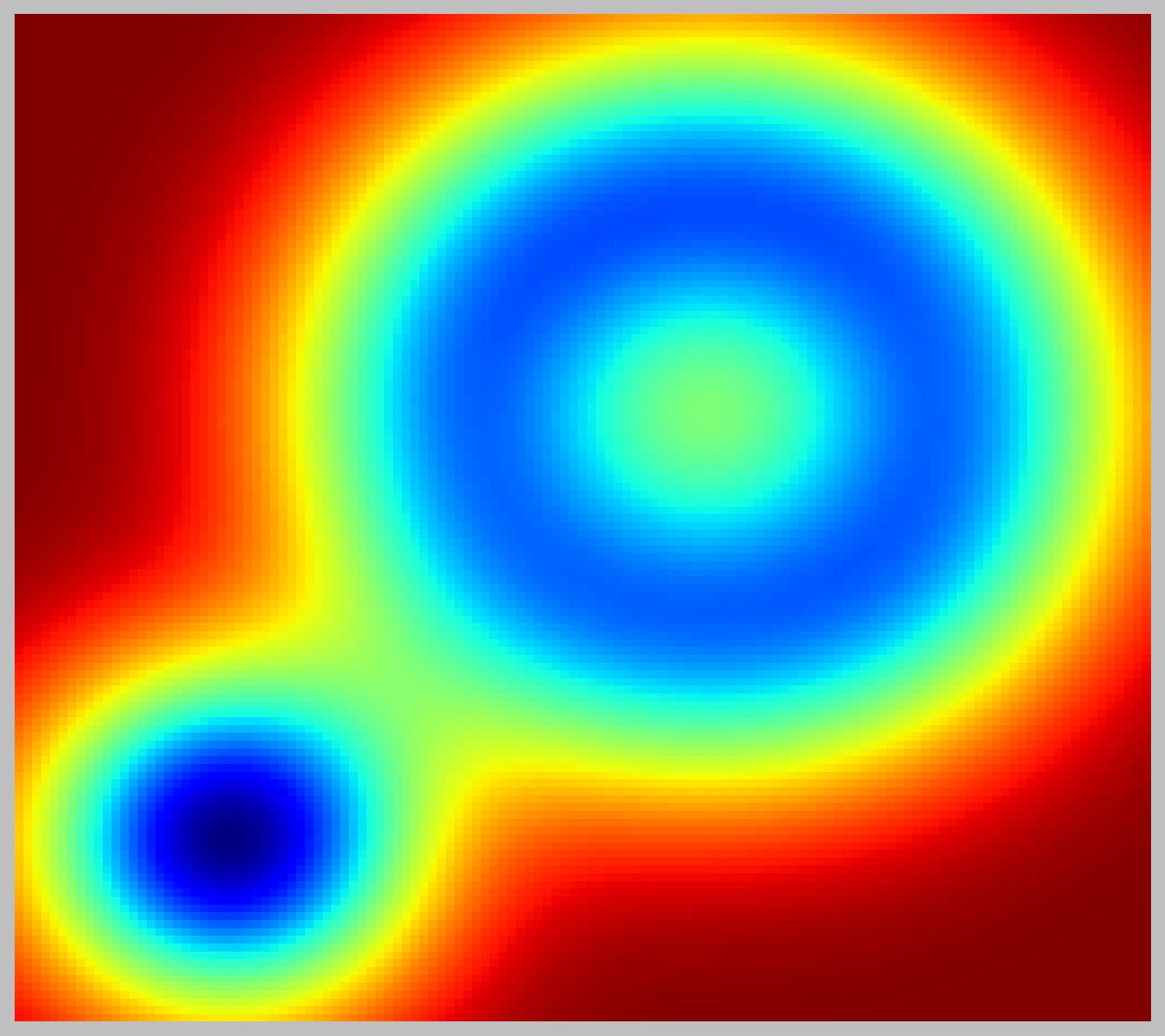
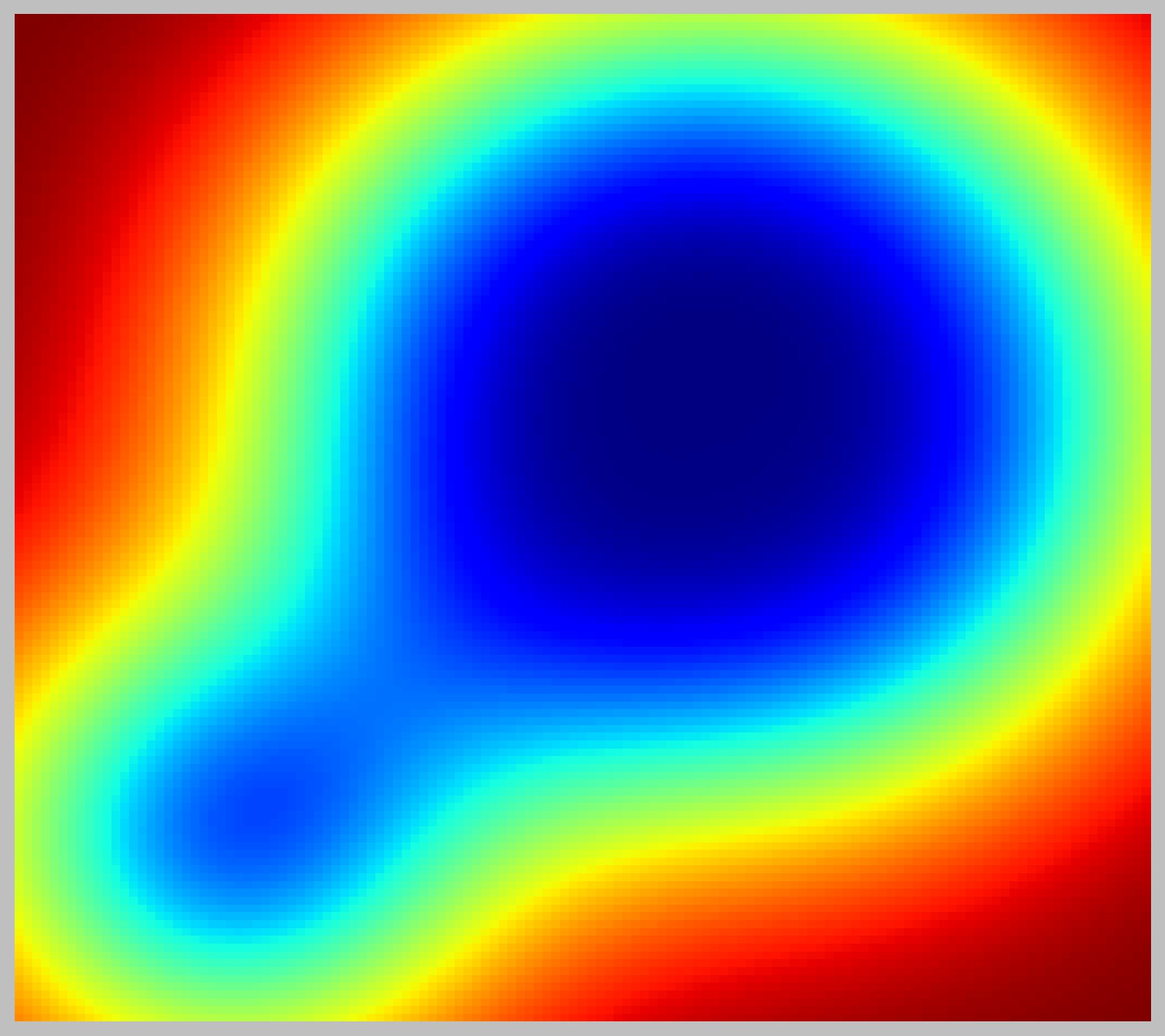
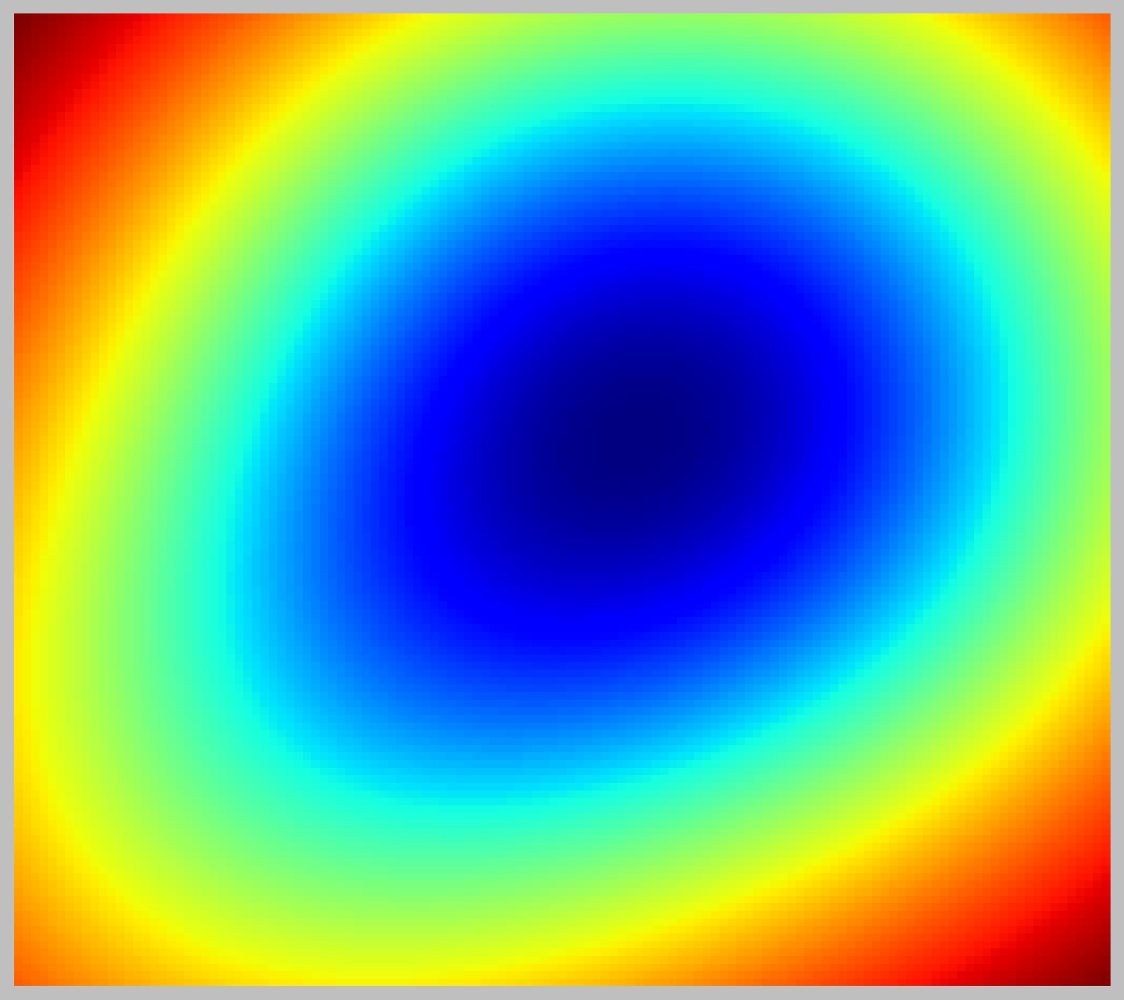
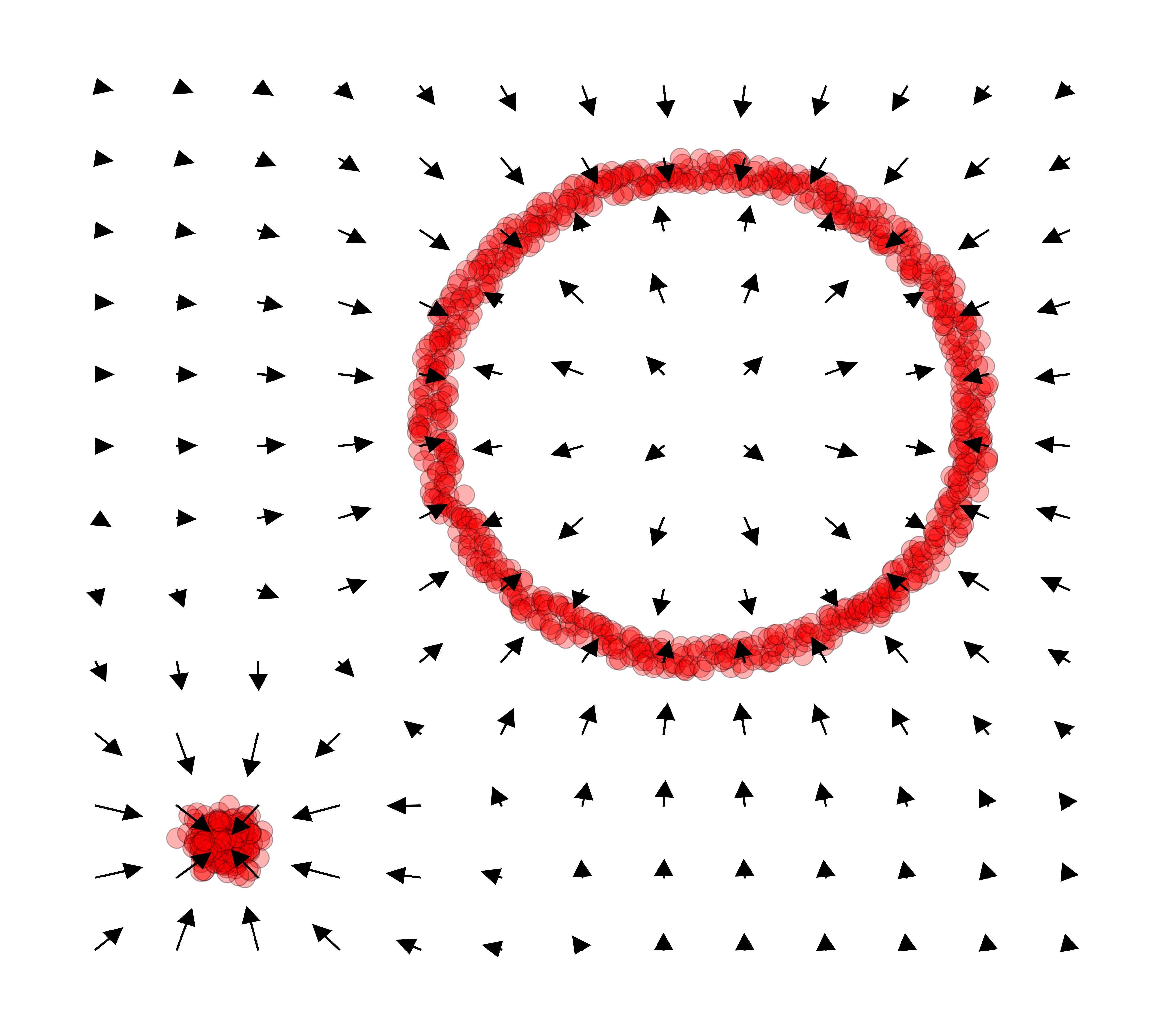
In this example, we consider the dataset formed by $n=1000$ points in $\mathbb{R}^{2}$, shown on the first panel of Figure 2. The other panels show the diffusion Fréchet functions for the corresponding empirical measure $\alpha_{n}$, calculated at increasing scales, and the gradient field $-\nabla V_{\alpha_{n}}$ at $t=2$, whose behavior reflects the organization of the data at that scale.

data $t=0.5$ $t=2$ $t=4.5$ $t=9$ $t=30$

$t=2$

Figure 2: Data points in $\mathbb{R}^{2}$, heat maps of their diffusion Fréchet functions at increasing scales, and the gradient field at $t=2$.

Example 3.

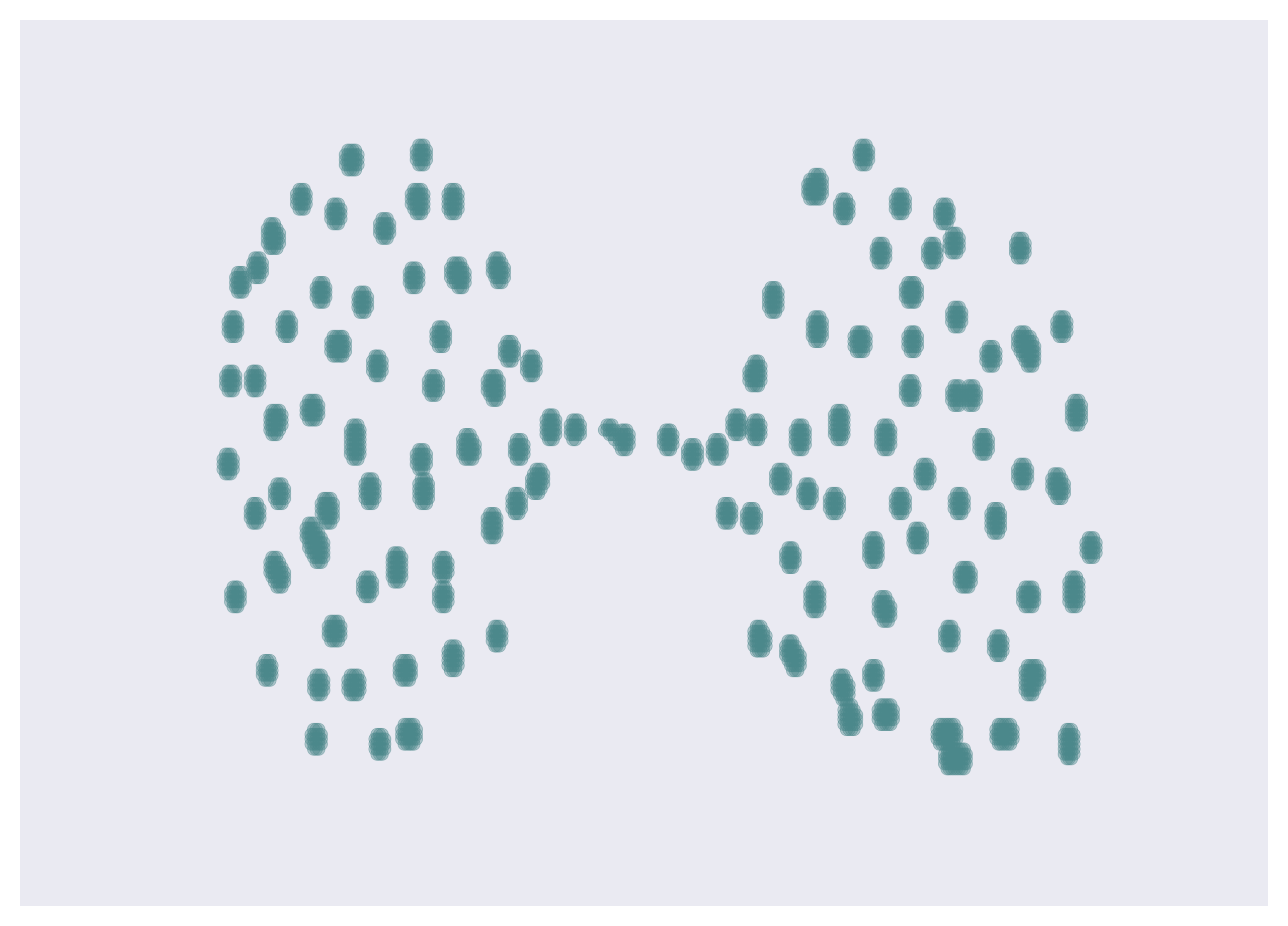
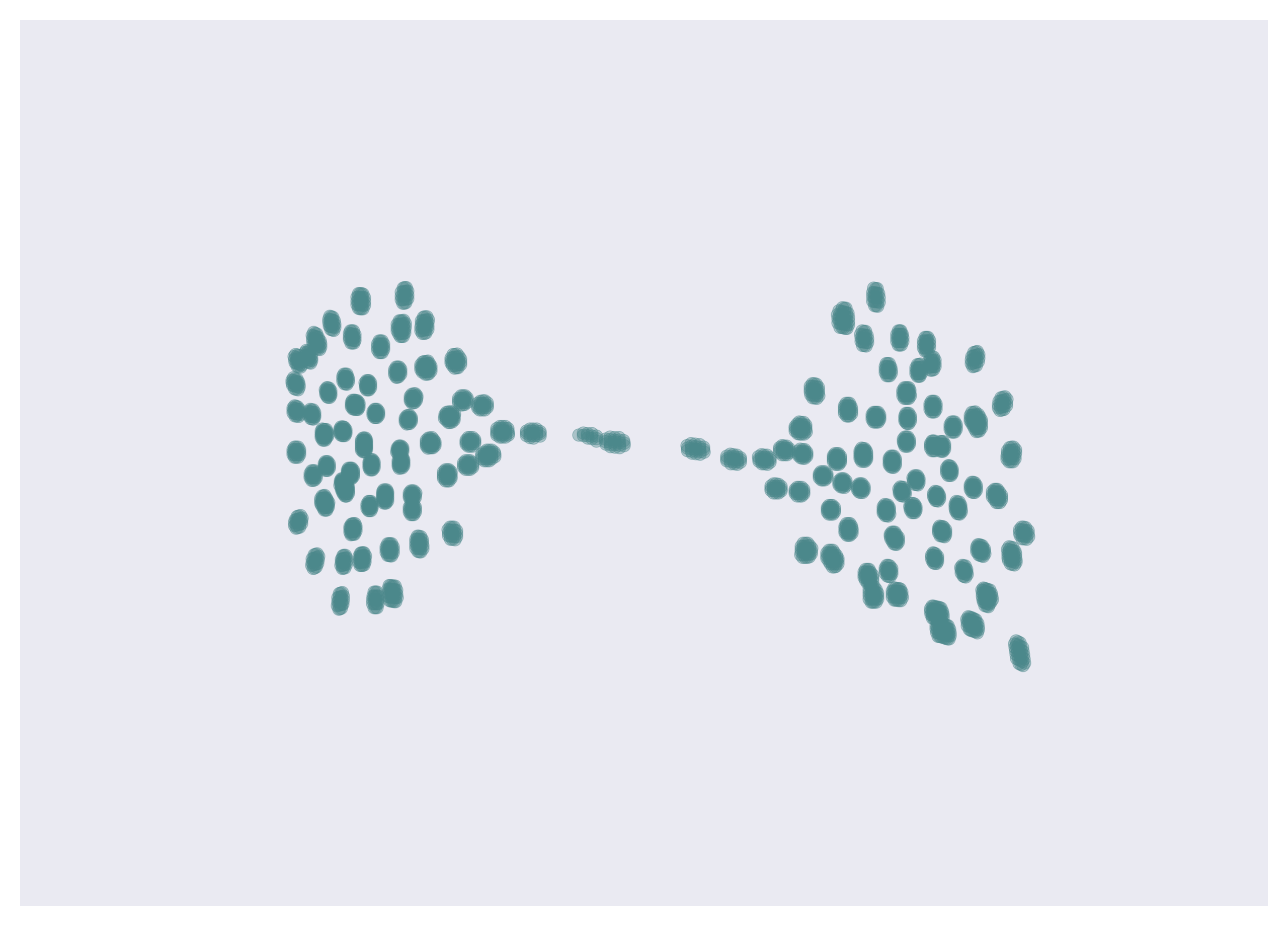
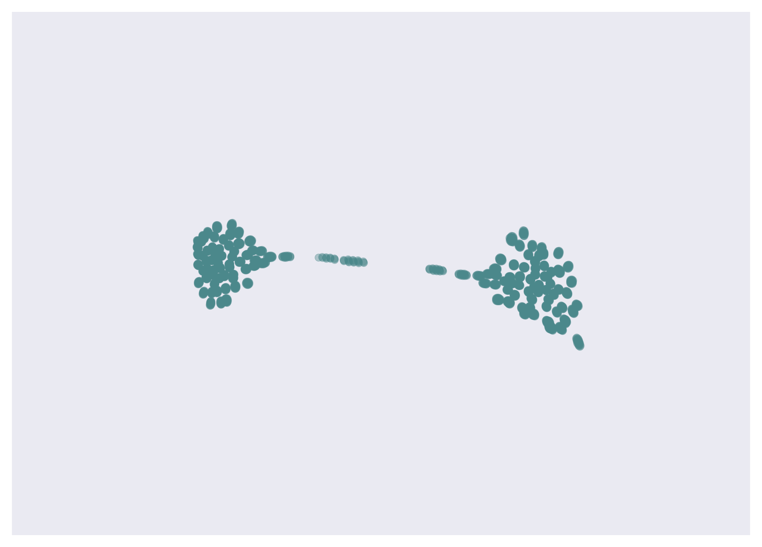
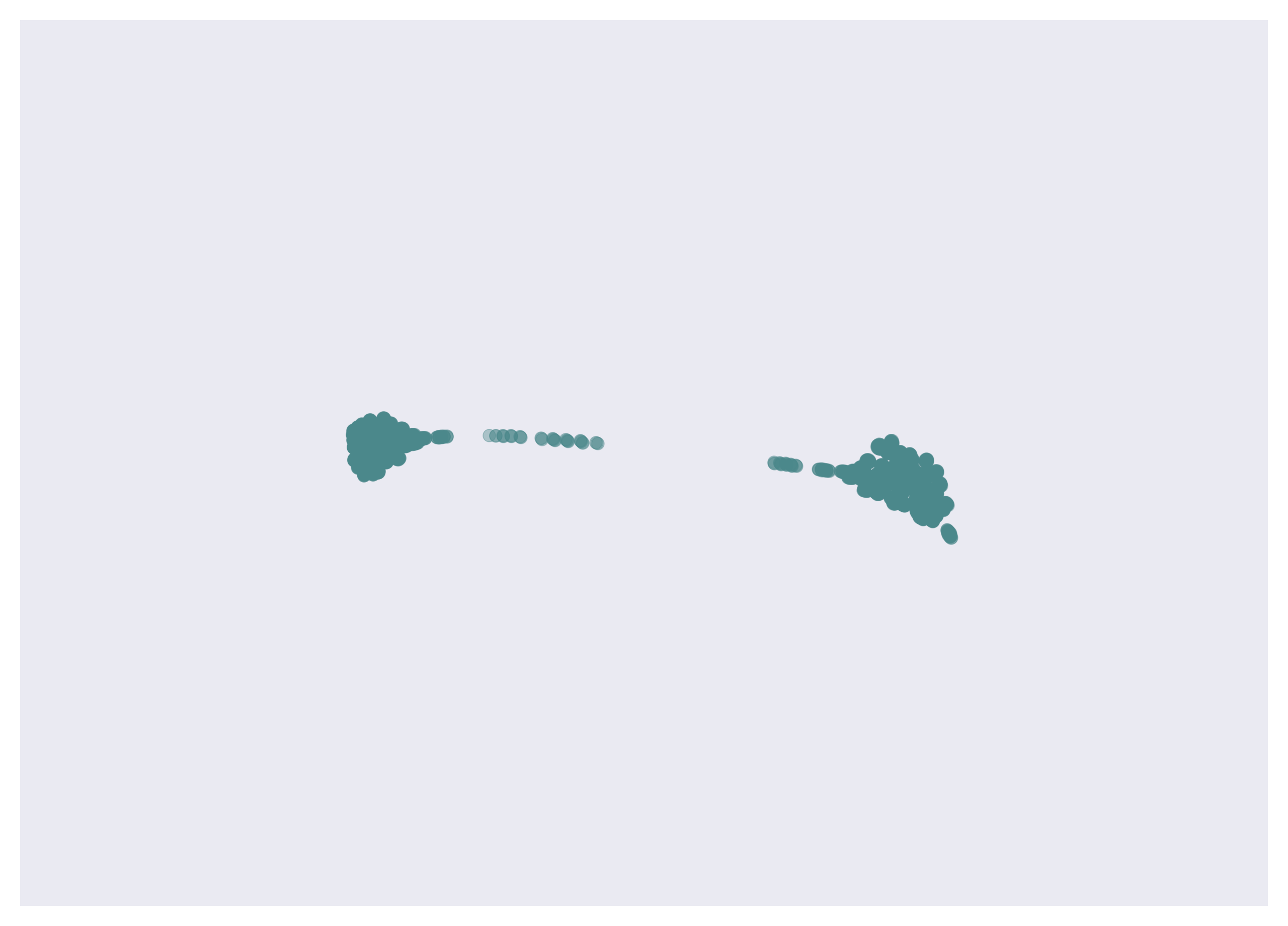
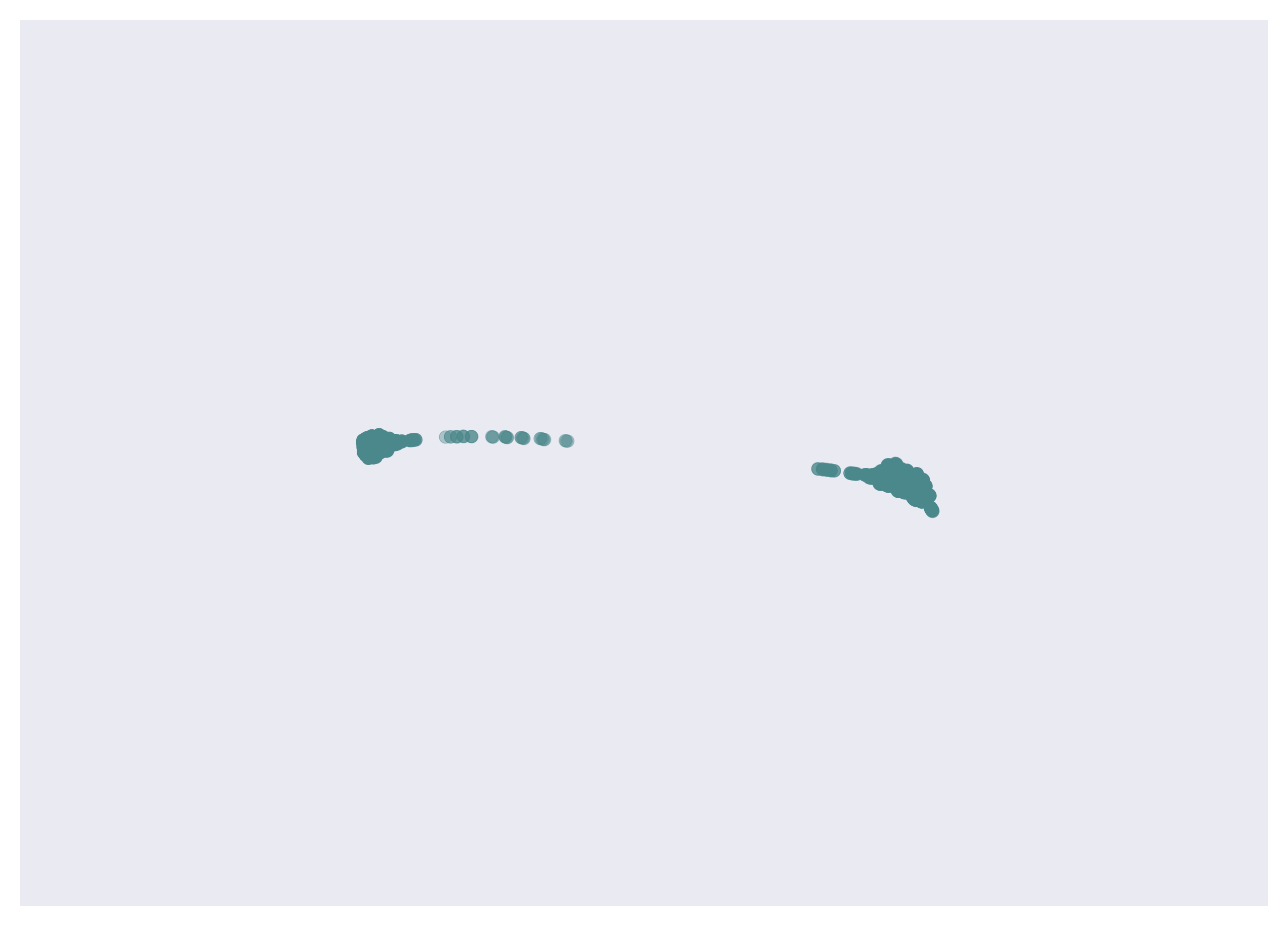
This example illustrates the evolution of a dataset consisting of $n=3158$ points under the (negative) gradient flow of the Fréchet function of the associated empirical measure at scale $t=0.2$. Panel (a) in Figure 3 shows the original data and the other panels show various stages of the evolution towards the attractors of the system.

(a)	(b)	(c)
(d)	(e)	(f)

Figure 3: Panel (a) shows the original data and panels (b)–(f) display various stages of the evolution of the data towards the attractors of the gradient flow of the Fréchet function at scale $t=0.2$.

We now prove stability results for $V_{\alpha,t}$ and its gradient field $\nabla V_{\alpha,t}$, which provide a basis for their use as robust functional statistics in data analysis. We begin by reviewing the definition of the Wasserstein distance between two probability measures.

A coupling between two probability measures $\alpha$ and $\beta$ is a probability measure $\mu$ on $\mathbb{R}^{d}\times\mathbb{R}^{d}$ such that $(p_{1})_{\ast}(\mu)=\alpha$ and $(p_{2})_{\ast}(\mu)=\beta$. Here, $p_{1}$ and $p_{2}$ denote the projections onto the first and second coordinates, respectively. The set of all such couplings is denoted $\Gamma(\alpha,\beta)$.

For each $p\in[1,\infty)$, let $\mathcal{P}_{p}(\mathbb{R}^{d})$ denote the collection of all Borel probability measures $\alpha$ on $\mathbb{R}^{d}$ whose $p$th moment $M_{p}(\alpha)=\int\|y\|^{p}\,d\alpha(y)$ is finite.

Definition 1 (cf.[2]).

Let $\alpha,\beta\in\mathcal{P}_{p}(\mathbb{R}^{d})$. The $p$-Wasserstein distance $W_{p}(\alpha,\beta)$ is defined as

$$W_{p}(\alpha,\beta)=\left(\inf_{\mu}\iint\limits_{\mathbb{R}^{d}\times\mathbb{R}^{d}}\|x-y\|^{p}d\mu(x,y)\right)^{1/p}\,,$$ (13)

where the infimum is taken over all $\mu\in\Gamma(\alpha,\beta)$.

It is well-known that the infimum in (13) is realized by some $\mu\in\Gamma(\alpha,\beta)$ [2]. Moreover, if $p>q\geq 1$, then $\mathcal{P}_{p}(\mathbb{R}^{d})\subset\mathcal{P}_{q}(\mathbb{R}^{d})$ and $W_{q}(\alpha,\beta)\leq W_{p}(\alpha,\beta)$.

The following lemma will be useful in the proof of the stability results. Part (a) of the lemma is a special case of Lemma 1 of [6]. Let $K_{t}\colon\mathbb{R}^{d}\to\mathbb{R}$ be the heat kernel centered at zero. In the notation used in (3), $K_{t}(y)=G_{t}(0,y)$.

Lemma 1.

Let $\displaystyle C_{d}(t)=(4\pi t)^{d/2}$. For any $y_{1},y_{2}\in\mathbb{R}^{d}$ and $t>0$, we have:

• $\displaystyle\left|K_{t}(y_{1})-K_{t}(y_{2})\right|\leq\frac{\|y_{1}-y_{2}\|}{C_{d}(t)\sqrt{2t\cdot e}}$ ;

• $\displaystyle\left\|y_{1}K_{t}(y_{1})-y_{2}K_{t}(y_{2})\right\|\leq\frac{e+2}{eC_{d}(t)}\|y_{1}-y_{2}\|$.

Proof.

(a) For each $\xi\in[0,1]$, let $y(\xi)=\xi y_{1}+(1-\xi)y_{2}$. Then,

$$\begin{split}\|K_{t}(y_{1})-K_{t}(y_{2})\|&=\left|\int_{0}^{1}\frac{d}{d\xi}K_{t}(y(\xi))\,d\xi\right|\leq\int_{0}^{1}\left|\frac{d}{d\xi}K_{t}(y(\xi))\right|\,d\xi\\ &=\int_{0}^{1}\left|\nabla K_{t}(y(\xi))\cdot(y_{1}-y_{2})\right|\,d\xi\\ &\leq\|y_{1}-y_{2}\|\int_{0}^{1}\left\|\nabla K_{t}(y(\xi))\right\|\,d\xi\,.\end{split}$$ (14)

Note that

$$\|\nabla K_{t}(y)\|=\|\frac{y}{2t}K_{t}(y)\|\leq\frac{\|y\|}{2tC_{d}(t)}\exp\left(-\frac{\|y\|^{2}}{4t}\right)\leq\frac{1}{C_{d}(t)\sqrt{2t\cdot e}}\,.$$ (15)

In the last inequality we used the fact that $\|y\|\exp\left(-\frac{\|y\|^{2}}{4t}\right)\leq\sqrt{\frac{2t}{e}}$. Hence,

$$\begin{split}\left|K_{t}(y_{1})-K_{t}(y_{2})\right|&\leq\frac{\|y_{1}-y_{2}\|}{C_{d}(t)\sqrt{2t\cdot e}}\,.\end{split}$$

(b) Using the same notation as in (a),

$$\frac{d}{d\xi}\left[yK_{t}(y)\right]=K_{t}(y)(y_{1}-y_{2})-y\frac{K_{t}(y)}{2t}\,y\cdot(y_{2}-y_{2})\,.$$ (16)

Hence,

$$\begin{split}\left\|\frac{d}{d\xi}\left[yK_{t}(y)\right]\right\|&\leq\left(K_{t}(y)+\frac{\|y\|^{2}}{2t}K_{t}(y)\right)\|y_{2}-y_{2}\|\\ &\leq\frac{1}{C_{d}(t)}\left(1+\frac{2}{e}\right)\|y_{1}-y_{2}\|\,.\end{split}$$ (17)

In the last inequality we used the facts that $K_{t}(y)\leq 1/C_{d}(t)$ and $\|y\|^{2}K_{t}(y)\leq 4t/eC_{d}(t)$. Writing

$$y_{1}K_{t}(y_{1})-y_{2}K_{t}(y_{2})=\int_{0}^{1}\frac{d}{d\xi}\left[yK_{t}(y)\right]\,d\xi\,,$$ (18)

it follows from (17) and (18) that

$$\|y_{1}K_{t}(y_{1})-y_{2}K_{t}(y_{2})\|\leq\frac{1}{C_{d}(t)}\left(1+\frac{2}{e}\right)\|y_{1}-y_{2}\|\,,$$ (19)

as claimed. ∎

Theorem 1 (Stability of Fréchet functions).

Let $\alpha$ and $\beta$ be Borel probability measures on $\mathbb{R}^{d}$ with diffusion Fréchet functions $V_{\alpha,t}$ and $V_{\beta,t}$, $t>0$, respectively. If $\alpha,\beta\in\mathcal{P}_{1}(\mathbb{R}^{d})$, then

$$\left\|V_{\alpha,t}-V_{\beta,t}\right\|_{\infty}\leq\frac{1}{C_{d}(2t)\sqrt{t\cdot e}}\,W_{1}(\alpha,\beta)\,.$$

Proof.

Fix $t>0$ and $x\in\mathbb{R}^{d}$. Let $\mu\in\Gamma(\alpha,\beta)$ be a coupling such that

$$\iint\limits_{\mathbb{R}^{d}\times\mathbb{R}^{d}}\|z_{1}-z_{2}\|d\mu(z_{1},z_{2})=W_{1}(\alpha,\beta)\,.$$ (20)

Then, we may write

$$V_{\alpha,t}(x)=\iint\limits_{\mathbb{R}^{d}\times\mathbb{R}^{d}}d^{2}_{t}(z_{1},x)\,d\mu(z_{1},z_{2})$$ (21)

and

$$V_{\beta,t}(x)=\iint\limits_{\mathbb{R}^{d}\times\mathbb{R}^{d}}d^{2}_{t}(z_{2},x)\,d\mu(z_{1},z_{2}).$$ (22)

By (6), $d^{2}_{t}(z,x)=2/C_{d}(2t)-2G_{2t}(z,x)$. Hence,

$$V_{\alpha,t}(x)-V_{\beta,t}(x)=-2\iint\limits_{\mathbb{R}^{d}\times\mathbb{R}^{d}}\left(G_{2t}(z_{1},x)-G_{2t}(z_{2},x)\right)d\mu(z_{1},z_{2})\,,$$ (23)

which implies that

$$\left|V_{\alpha,t}(x)-V_{\beta,t}(x)\right|\leq 2\iint\limits_{\mathbb{R}^{d}\times\mathbb{R}^{d}}\left|G_{2t}(z_{1},x)-G_{2t}(z_{2},x)\right|d\mu(z_{1},z_{2})\,.$$ (24)

After translating $\alpha$ and $\beta$, we may assume that $x=0$. Thus, by Lemma 1(a),

$$\begin{split}\left|V_{\alpha,t}(x)-V_{\beta,t}(x)\right|&\leq\frac{1}{C_{d}(2t)\sqrt{t\cdot e}}\iint\limits_{\mathbb{R}^{d}\times\mathbb{R}^{d}}\left\|z_{1}-z_{2}\right\|d\mu(z_{1},z_{2})\\ &=\frac{1}{C_{d}(2t)\sqrt{t\cdot e}}\,W_{1}(\alpha,\beta)\,,\end{split}$$ (25)

as claimed. ∎

Theorem 2 (Stability of gradient fields).

Let $\alpha$ and $\beta$ be Borel probability measures on $\mathbb{R}^{d}$ with diffusion Fréchet functions $V_{\alpha,t}$ and $V_{\beta,t}$, $t>0$, respectively. If $\alpha,\beta\in\mathcal{P}_{1}(\mathbb{R}^{d})$, then

$$\sup_{x\in\mathbb{R}^{d}}\left\|\nabla V_{\alpha,t}(x)-\nabla V_{\beta,t}(x)\right\|\leq\frac{e+2}{eC_{d}(2t)}\,W_{1}(\alpha,\beta)\,.$$

Proof.

Let $\mu\in\Gamma(\alpha,\beta)$ be a coupling that realizes $W_{1}(\alpha,\beta)$. From (23), it follows that

$$\begin{split}\|\nabla V_{\alpha,t}(x)&-\nabla V_{\beta,t}(x)\|\leq 2\iint\left\|\nabla_{x}G_{2t}(z_{1},x)-\nabla_{x}G_{2t}(z_{2},x)\right\|d\mu(z_{1},z_{2})\\ &\leq\frac{1}{2t}\iint\limits\left\|(x-z_{1})G_{2t}(z_{1},x)-(x-z_{2})G_{2t}(z_{2},x)\right\|d\mu(z_{1},z_{2})\,.\end{split}$$ (26)

We may assume that $x=0$, so we rewrite the previous inequality as

$$\|\nabla V_{\alpha,t}(x)-\nabla V_{\beta,t}(x)\|\leq\frac{1}{2t}\iint\left\|z_{1}K_{2t}(z_{1})-z_{2}K_{2t}(z_{2})\right\|d\mu(z_{1},z_{2})\,.$$ (27)

Therefore, by Lemma 1(b),

$$\begin{split}\|\nabla V_{\alpha,t}(x)-\nabla V_{\beta,t}(x)\|&\leq\frac{e+2}{eC_{d}(2t)}\iint\|z_{1}-z_{2}\|d\mu(z_{1},z_{2})\\ &=\frac{e+2}{eC_{d}(2t)}W_{1}(\alpha,\beta)\,,\end{split}$$ (28)

which proves the theorem. ∎

4 Diffusion Fréchet Vectors on Networks

In this section, we define a network analogue of diffusion Fréchet functions and prove a stability theorem. Let $\xi=[\xi_{1}\,\ldots\,\xi_{n}]^{T}\in\mathbb{R}^{n}$ represent a probability distribution on the vertex set $V=\{v_{1},\ldots,v_{n}\}$ of a weighted network $K$. For $t>0$, define the diffusion Fréchet vector (DFV) as the vector $F_{\xi,t}\in\mathbb{R}^{n}$ whose $i$th component is

$$F_{\xi,t}(i)=\sum_{j=1}^{n}d_{t}^{2}(i,j)\xi_{j}\,.$$ (29)

Example 4.

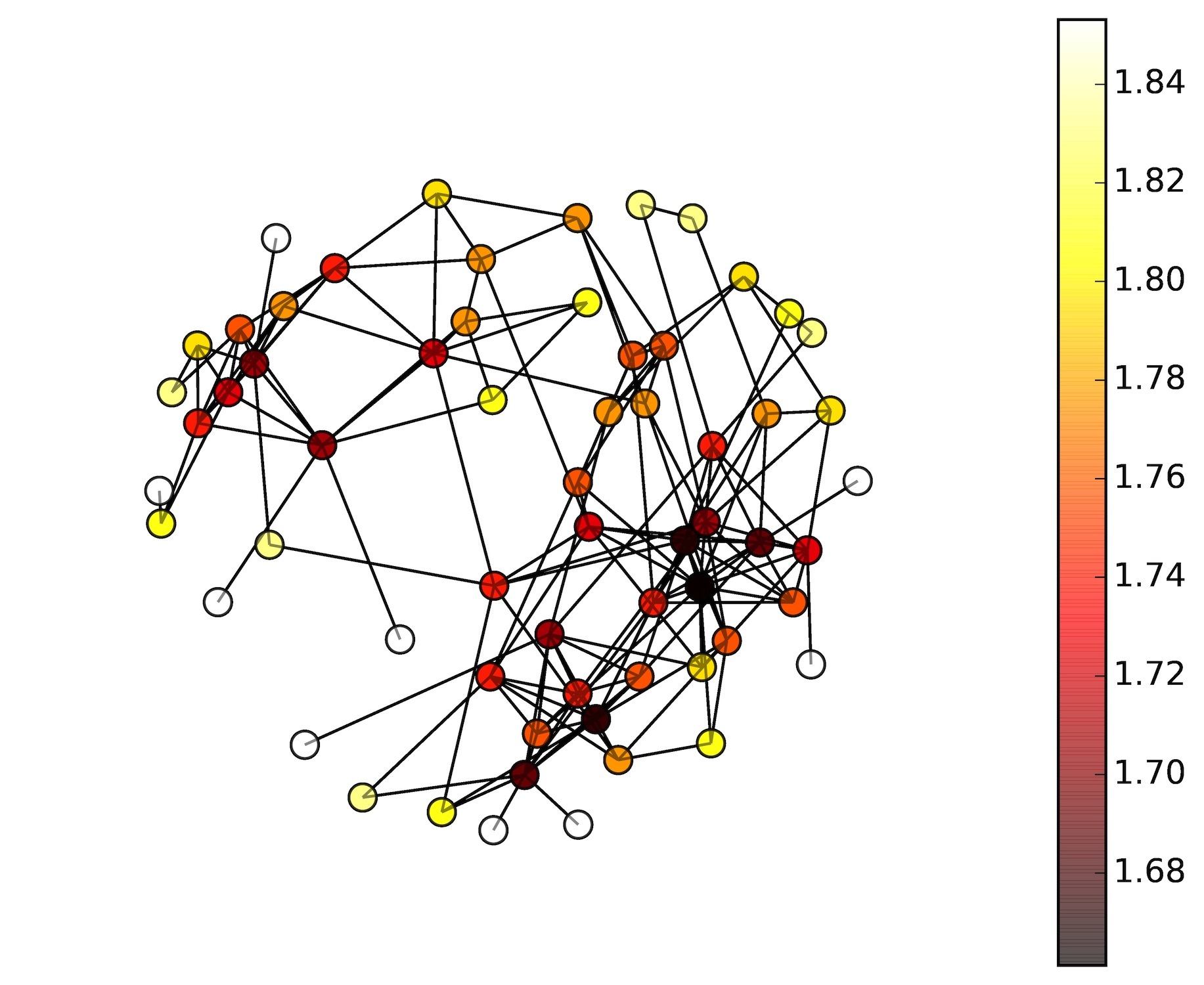
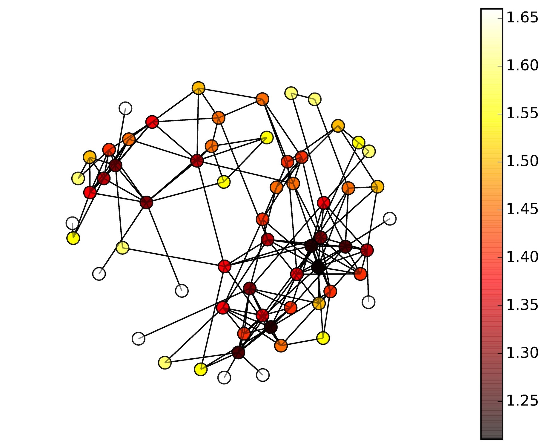
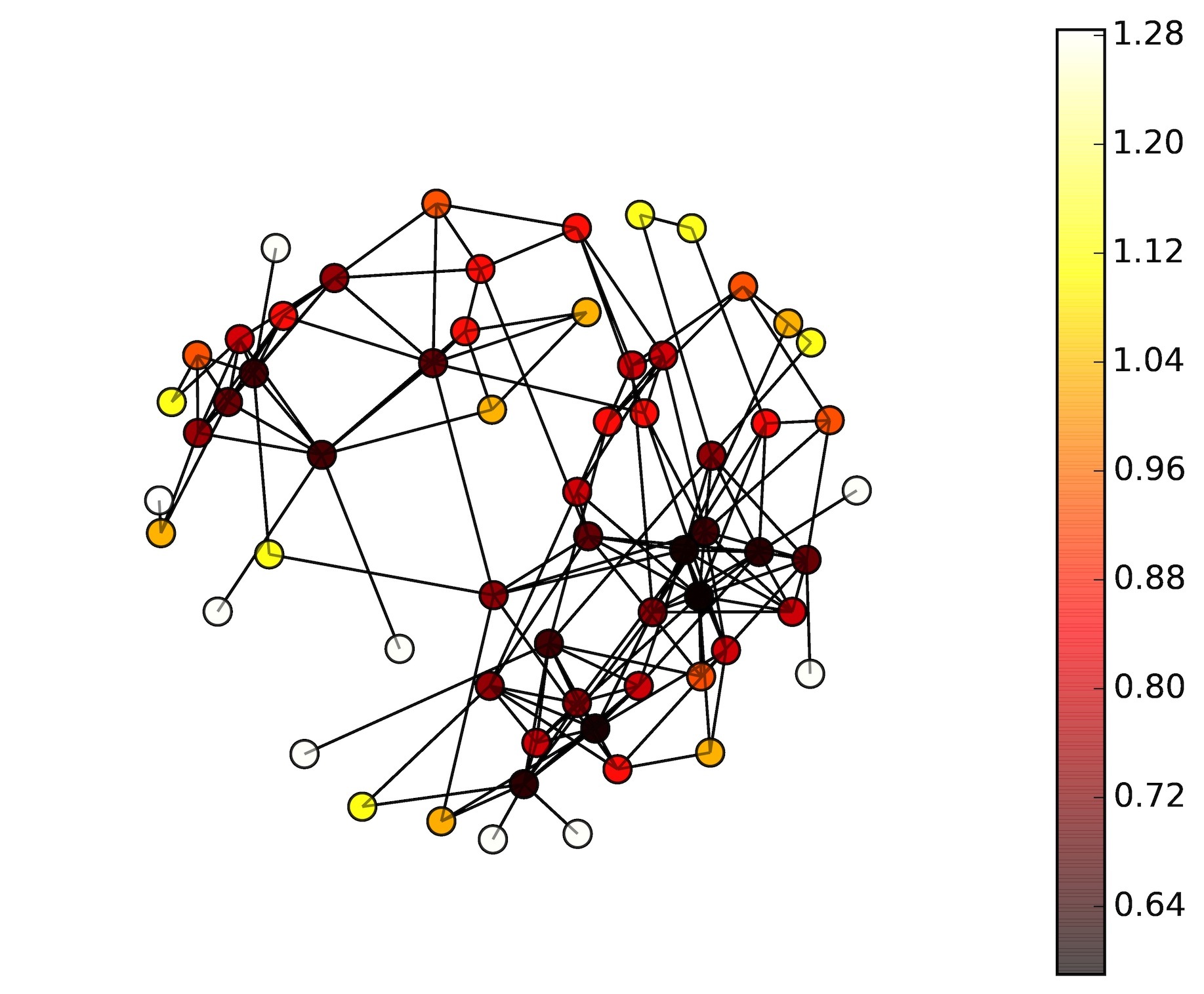
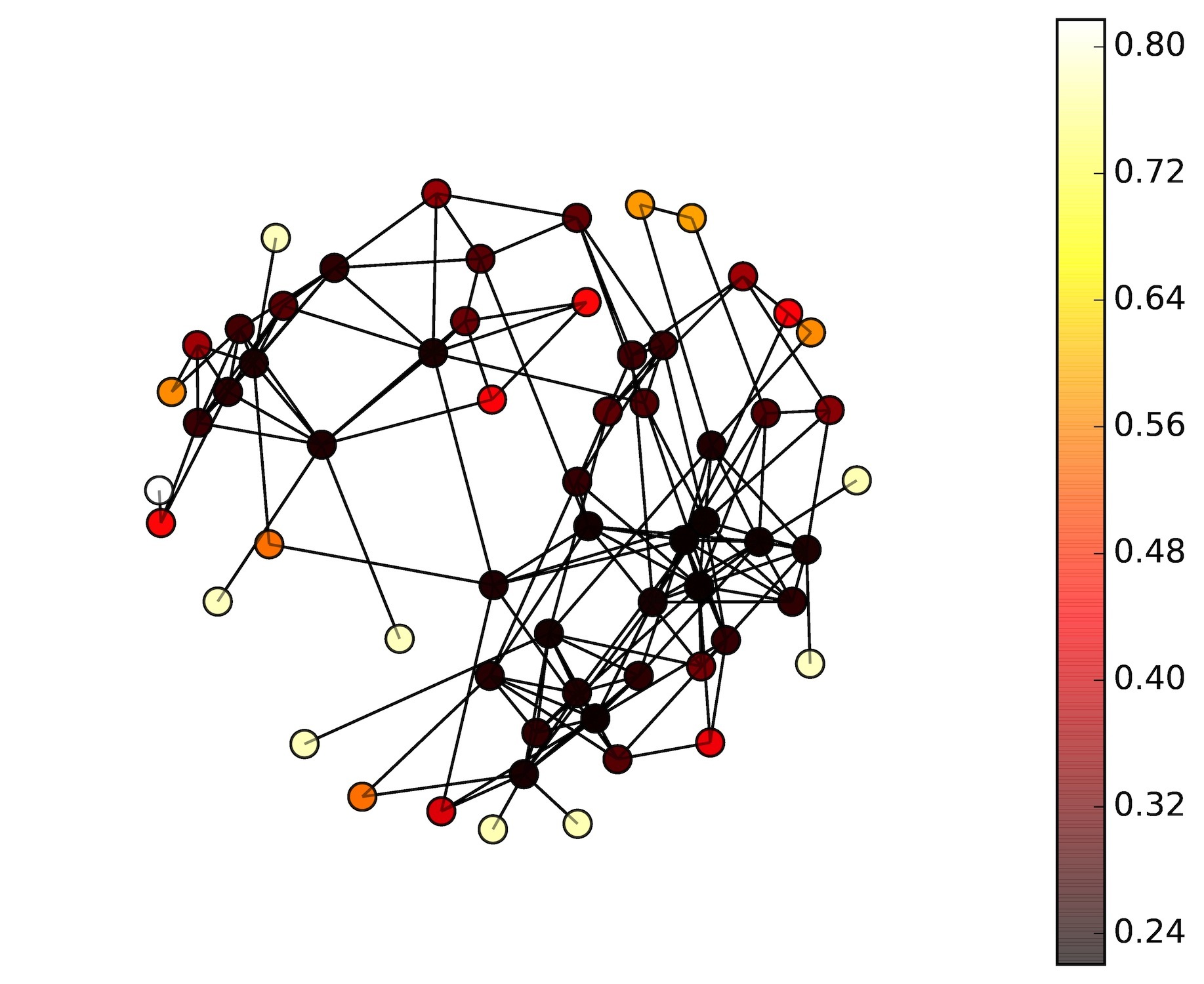
We illustrate the behavior of DFVs on a social network of frequent interactions among 62 dolphins in a community living off Doubtful Sound, New Zealand [7]. The network data was obtained from the UC Irvine Network Data Repository. All edges are given the same weight and we consider the uniform distribution on the vertex set. Figure 4 shows maps of the diffusion Fréchet vector at multiple scales. As in the Euclidean case, the profiles of the DFVs reveal sub-communities in the network and their interactions.

$t=0.01$	$t=0.03$
$t=0.09$	$t=0.3$

Figure 4: Evolution across scales of the diffusion Fréchet vector for the uniform distribution.

To state a stability theorem for DFVs, we first define the Wasserstein distance between two probability distributions on the vertex set $V$ of a weighted network $K$. This requires a base metric on $V$ to play a role similar to that of the Euclidean metric in (13). We use the commute-time distance between the nodes of a weighted network (cf. [8]).

Definition 2.

Let $K$ be a connected, weighted network with nodes $v_{1},\ldots,v_{n}$, and let $\phi_{1},\phi_{2},\ldots,\phi_{n}$ be an orthonormal basis of $\mathbb{R}^{n}$ formed by eigenvectors of the graph Laplacian with eigenvalues $0=\lambda_{1}<\lambda_{2}\leq\ldots\leq\lambda_{n}$. The commute-time distance between $v_{i}$ and $v_{j}$ is defined as

$$d_{CT}(i,j)=\left(\sum_{k=2}^{n}\frac{1}{\lambda_{k}}\left(\phi_{k}(i)-\phi_{k}(j)\right)^{2}\right)^{1/2}.$$ (30)

It is simple to verify that $d_{CT}^{2}(i,j)=2\int_{0}^{\infty}d_{t}^{2}(i,j)\,dt$.

Definition 3.

Let $\xi,\zeta\in\mathbb{R}^{n}$ represent probability distributions on $V$. The $p$-Wasserstein distance, $p\geq 1$, between $\xi$ and $\zeta$ (with respect to the commute-time distance on $V$) is defined as

$$W_{p}(\xi,\zeta)=\min_{\mu\in\Gamma(\alpha,\beta)}\left(\sum_{j=1}^{n}\sum_{i=1}^{n}d_{CT}^{p}(i,j)\mu_{ij}\right)^{1/p}\,,$$ (31)

where $\Gamma(\xi,\zeta)$ is the set of all probability measures $\mu$ on $V\times V$ satisfying $(p_{1})_{\ast}(\mu)=\xi$ and $(p_{2})_{\ast}(\mu)=\zeta$.

Theorem 3.

Let $\xi,\zeta\in\mathbb{R}^{n}$ be probability distributions on the vertex set of a connected, weighted network. For each $t>0$, their diffusion Fréchet vectors satisfy

$$\|F_{\xi,t}-F_{\zeta,t}\|_{\infty}\leq 4\sqrt{\frac{\operatorname{Tr}e^{-2t\Delta}-1}{2et}}\,W_{1}(\xi,\zeta)\,.$$ (32)

Proof.

Fix $t>0$ and a node $v_{\ell}$. Let $\mu\in\Gamma(\xi,\zeta)$ be such that

$$\sum_{j=1}^{n}\sum_{i=1}^{n}d_{CT}(i,j)\mu(i,j)=W_{1}(\xi,\zeta)\,.$$ (33)

Since $\mu$ has marginals $\alpha$ and $\beta$, we may write

$$F_{\xi,t}(\ell)=\sum_{j=1}^{n}\sum_{i=1}^{n}d_{t}^{2}(i,\ell)\mu_{i,j}\quad\text{and}\quad F_{\zeta,t}(\ell)=\sum_{j=1}^{n}\sum_{i=1}^{n}d_{t}^{2}(j,\ell)\mu_{i,j}\,,$$ (34)

which implies that

$$\left|F_{\xi,t}(\ell)-F_{\zeta,t}(\ell)\right|\leq\sum_{j=1}^{n}\sum_{i=1}^{n}\left|d_{t}^{2}(i,\ell)-d_{t}^{2}(j,\ell)\right|\mu_{i,j}\,.$$ (35)

By Lemma 2 below,

$$\begin{split}\left|F_{\xi,t}(\ell)-F_{\zeta,t}(\ell)\right|\leq&4\sqrt{\operatorname{Tr}e^{-2\Delta t}-1}\sum_{j=1}^{n}\sum_{i=1}^{n}d_{t}(i,j)\mu_{i,j}\,.\end{split}$$ (36)

Observe that

$$\begin{split}d_{t}^{2}(i,j)&=\sum_{k=1}^{n}e^{-2\lambda_{k}t}\left(\phi_{k}(i)-\phi_{k}(j)\right)^{2}\\ &=\sum_{k=1}^{n}\lambda_{k}e^{-2\lambda_{k}t}\frac{1}{\lambda_{k}}\left(\phi_{k}(i)-\phi_{k}(j)\right)^{2}\leq\frac{1}{2et}d_{CT}^{2}(i,j)\end{split}$$ (37)

since $\lambda_{k}e^{-2\lambda_{k}t}\leq\frac{1}{2et}$. The theorem follows from (36) and (37). ∎

Lemma 2.

Let $v_{i},v_{j},v_{\ell}$ be nodes of a connected, weighted network. For any $t>0$,

$$\left|d_{t}^{2}(i,\ell)-d_{t}^{2}(j,\ell)\right|\leq 4\sqrt{\operatorname{Tr}e^{-2t\Delta}-1}\,d_{t}(i,j)\,,$$

where $\operatorname{Tr}$ denotes the trace operator.

Proof.

Since the eigenfunction $\phi_{1}$ is constant, we may write the diffusion distance as

$$\begin{split}d_{t}^{2}(i,\ell)=\sum_{k=2}^{n}e^{-2\lambda_{k}t}\left(\phi_{k}^{2}(i)-2\phi_{k}(i)\phi_{k}(\ell)+\phi_{k}^{2}(\ell)\right)\,.\end{split}$$ (38)

Thus,

$$\begin{split}d_{t}^{2}(i,\ell)-d_{t}^{2}(j,\ell)&=\sum_{k=2}^{n}e^{-2\lambda_{k}t}\left(\phi_{k}^{2}(i)-\phi_{k}^{2}(j)\right)\\ &-2\sum_{k=2}^{n}e^{-2\lambda_{k}t}\phi_{k}(\ell)\left(\phi_{k}(i)-\phi_{k}(j)\right)\\ &=\sum_{k=2}^{n}e^{-2\lambda_{k}t}(\phi_{k}(i)+\phi_{k}(j))(\phi_{k}(i)-\phi_{k}(j))\\ &-2\sum_{k=2}^{n}e^{-2\lambda_{k}t}\phi_{k}(\ell)\left(\phi_{k}(i)-\phi_{k}(j)\right)\,.\end{split}$$ (39)

Since each $\phi_{k}$ has unit norm, $|\phi_{k}(\ell)|\leq 1$ and $|\phi_{k}(i)+\phi_{k}(j)|\leq 2$  . Therefore,

$$\left|d_{t}^{2}(i,\ell)-d_{t}^{2}(j,\ell)\right|\leq 4\sum_{k=2}^{n}e^{-2\lambda_{k}t}\left|\phi_{k}(i)-\phi_{k}(j)\right|\,.$$ (40)

The Cauchy-Schwarz inequality, applied to the vectors $a=\left(e^{-\lambda_{2}t},\ldots,e^{-\lambda_{n}t}\right)$ and $b=\left(e^{-\lambda_{2}t}\left|\phi_{2}(i)-\phi_{2}(j)\right|,\ldots,e^{-\lambda_{n}t}\left|\phi_{n}(i)-\phi_{n}(j)\right|\right)$, yields

$$\begin{split}\sum_{k=2}^{n}e^{-2\lambda_{k}t}\left|\phi_{k}(i)-\phi_{k}(j)\right|&\leq\sqrt{\sum_{k=2}^{n}e^{-2\lambda_{k}t}}\,\sqrt{\sum_{k=2}^{n}e^{-2\lambda_{k}t}\left(\phi_{k}(i)-\phi_{k}(j)\right)^{2}}\\ &=\sqrt{\operatorname{Tr}e^{-2t\Delta}-1}\,d_{t}(i,j)\,.\end{split}$$ (41)

The lemma follows from (40) and (41). ∎

5 C. difficile Infection and Fecal Microbiota Transplantation

This section presents an application to analyses of microbiome data associated with Clostridium difficile infection (CDI). CDI kills thousands of patients every year in healthcare facilities [9]. Traditionally, CDI is treated with antibiotics, but the drugs also attack other bacteria in the gut flora and this has been linked to recurrence of CDI in recovering patients [10]. Fecal microbiota transplantation (FMT) is a promising alternative that shows recovery rates close to $90\%$ [11, 12]. Shahinas et al. [13] and Seekatz et al. [14] have used 16S rRNA sequencing to estimate the abundance of the various bacterial taxa living in the gut of healthy donors and CDI patients. These studies have reported a reduced diversity in the bacterial communities of CDI patients and abundance scores after FMT treatment that are closer to those for healthy donors. The studies, however, have focused on counts of bacterial taxa, disregarding interactions in the bacterial communities. To account for these, we employ diffusion Fréchet vectors to examine differences in pre-treatment and post-treatment fecal samples and the effect of FMT in the composition of the gut flora. The analysis is based on metagenomic data for 17 patients (paired pre-FMT and post-FMT) and 7 donor samples, selected from data collected by Lee et al. [15].

5.1 Metagenomic Data

The data comes from a subset of 94 patients treated with fecal microbiota transplantation by one of the authors [15], covering the period 2008–2012. From this, 17 patients were selected, not randomly, for sequencing. The protocol followed for obtaining consent consisted of first sending a written letter to each patient asking permission to further study their already collected stool samples. In the letter it was stated that there will be a followup telephone call to the patient verifying that they received the letter and whether they will provide consent 5-10 business days following the date of the mailing. All patients in this study were contacted, and all patients provided written informed consent. Furthermore, this study and permission protocol was approved by the Hamilton Integrated Research Ethics Board #12-3683, the University of Guelph Research Ethics Board 12AU013 and the Florida State University Research Ethics IRB00000446.

All C. difficile infections were confirmed by in-hospital, real-time, polymerase chain reaction (PCR) testing for the toxin B gene. This study sequenced the forward V3-V5 region of the 16S rRNA gene from 17 CDI patients who were treated with FMT(s). A pre-FMT, a corresponding post-FMT, and 7 samples from four donors, corresponding altogether to 41 fecal samples were sequenced.

The bioinformatics software mothur was used as the primary means of processing and quality-filtering reads and calculating statistical indices of community structure; see [16] for a breakdown of the mothur processing pipeline.

5.2 Co-occurrence Networks

This study is based on bacterial interactions at the phylum level. We model the (expected) interactions among the various phyla found in the healthy human gut by means of a co-occurrence network [17] in which each node represents a phylum. An edge between two phyla is weighted according to the correlation between their counts, estimated from samples taken from a group of healthy individuals. More precisely, let $v_{1},\ldots,v_{n}$ be the nodes of the network and $\rho_{ij}$, $i\neq j$, be the correlation coefficient between the counts for the phyla represented by $v_{i}$ and $v_{j}$. As we are interested in sub-communities of interactive phyla, the edge between $v_{i}$ and $v_{j}$ is weighted by the absolute correlation $w_{ij}=|\rho_{ij}|$, disregarding whether the correlation is positive or negative. Since this construction typically yields a fully connected network, we use the locally adaptive network sparsification (LANS) technique [18] to simplify the network, retaining the most significant interactions (edges) while keeping the network connected. The following description of LANS is equivalent to that in [18]. Define

$$F_{ij}=\frac{1}{n}\sum_{k=1}^{n}\mathbf{1}\{w_{ik}\leqslant w_{ij}\}\,,$$ (42)

where $\mathbf{1}\{w_{ik}\leqslant w_{ij}\}$ returns $1$ if $w_{ik}\leqslant w_{ij}$ and $0$ otherwise. For a given pair $(i,j)$, $F_{ij}$ is the probability that the absolute correlation between the counts for a random phylum and $v_{i}$ is no larger than $w_{ij}$. Observe that $F_{ij}$ may differ from $F_{ji}$. For $i\neq j$, the decision as to whether the edge between $v_{i}$ and $v_{j}$ is deleted or preserved is based on a “significance” level $0\leqslant\alpha\leqslant 1$. The edge is preserved if $1-F_{ij}<\alpha$ or $1-F_{ji}<\alpha$. Larger values of $\alpha$ retain more edges of the network.

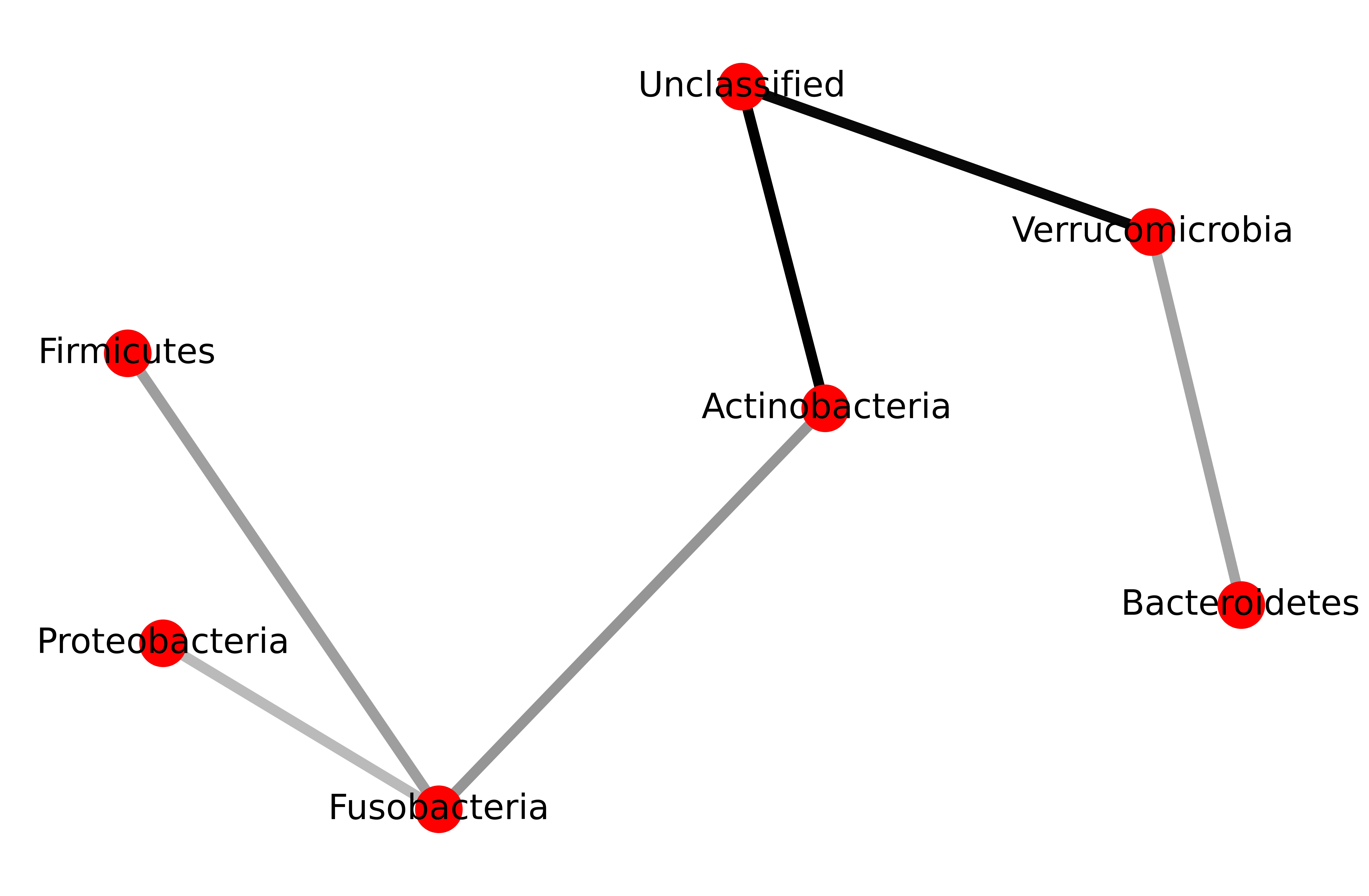
The model we develop is based on seven bacterial phyla: Actinobacteria, Bacteroidetes, Firmicutes, Fusobacteria, Proteobacteria, Verrucomicrobia, and a group of unidentified bacteria treated as a single phylum labeled Unclassified. Figure 5 shows the co-ocurrence network obtained after LANS sparsification with $\alpha=0.1$. Dark edge colors indicate a higher level of interaction; that is, larger edge weights. Note that there is a highly interactive sub-community comprising Actinobacteria, Verrucomicrobia and unclassified bacteria. This network is used in our analyses of variation in the structure of bacterial communities in samples from CDI patients, recovering patients and healthy individuals, as well as the effects of FMT. (The package NetworkX for the Python programming language was used to depict the network [19].)

Figure 5: Bacterial phyla co-occurrence network for the human gut sparsified to significance level $\alpha=0.1$ with the LANS method.

5.3 Microbiota Analysis

The co-occurrence network constructed in Section 5.2 (Figure 5) from culture data for healthy donors provides a model for the expected interactions among the seven bacterial phyla considered in this study. We use the network and bacterial count data to produce a biomarker $\gamma_{t}$ that is effective in characterizing CDI and potentially in monitoring the effects of FMT treatment. To establish a baseline, we also construct a biomarker $\beta$ solely based on bacterial counts and compare it with $\gamma_{t}$.

Let $v_{1},\ldots,v_{7}$ be the nodes of the co-occurrence network. For a gut culture sample $S$, let $\xi_{i}(S)$ be the frequency of $v_{i}$ in $S$. Clearly, $\xi_{1}(S)+\ldots+\xi_{7}(S)=1$. Our first method of analysis is based directly on the probability distribution on the vertex set given by

$$\xi(S)=\left(\xi_{1}(S),\ldots,\xi_{7}(S)\right)\in\mathbb{R}^{7}\,.$$ (43)

To derive a scalar biomarker $\beta(S)$, we use culture samples from healthy individuals and CDI patients. We calculate their 7-dimensional frequency vectors $\xi(S)$ and use linear discriminant analysis (LDA) to learn an axis in $\mathbb{R}^{7}$ along which their scores $\beta(S)$ optimally discriminate healthy samples from those of CDI patients. For a sample $S$, $\beta(S)$ is the score of $\xi(S)$ along the learned axis. Next, we describe the biomarker $\gamma_{t}$. For a sample $S$, let

$$F^{S}_{t}(i)=\sum_{j=1}^{7}d^{2}_{t}(i,j)\xi_{j}(S)$$ (44)

be the diffusion Fréchet vector for the distribution $\xi(S)$. As before, using training data and applying LDA, we obtain $\gamma_{t}$.

5.4 Results

Our analyses were based on 41 gut culture samples comprising 7 healthy donors, 17 pre-treatment CDI patients (pre-FMT), 4 post-treatment patients not in resolution (post-NR), and 13 post-treatment patients in resolution (post-R). Figure 6 shows boxplots for each of the four groups of the distribution of the phylum frequency data obtained from metagenomic sequencing of the forty-one samples.

Figure 6: Boxplot of bacterial phylum frequency in the human gut for healthy donors, pre-FMT patients, post-FMT patients not in resolution, and post-FMT patients in resolution.

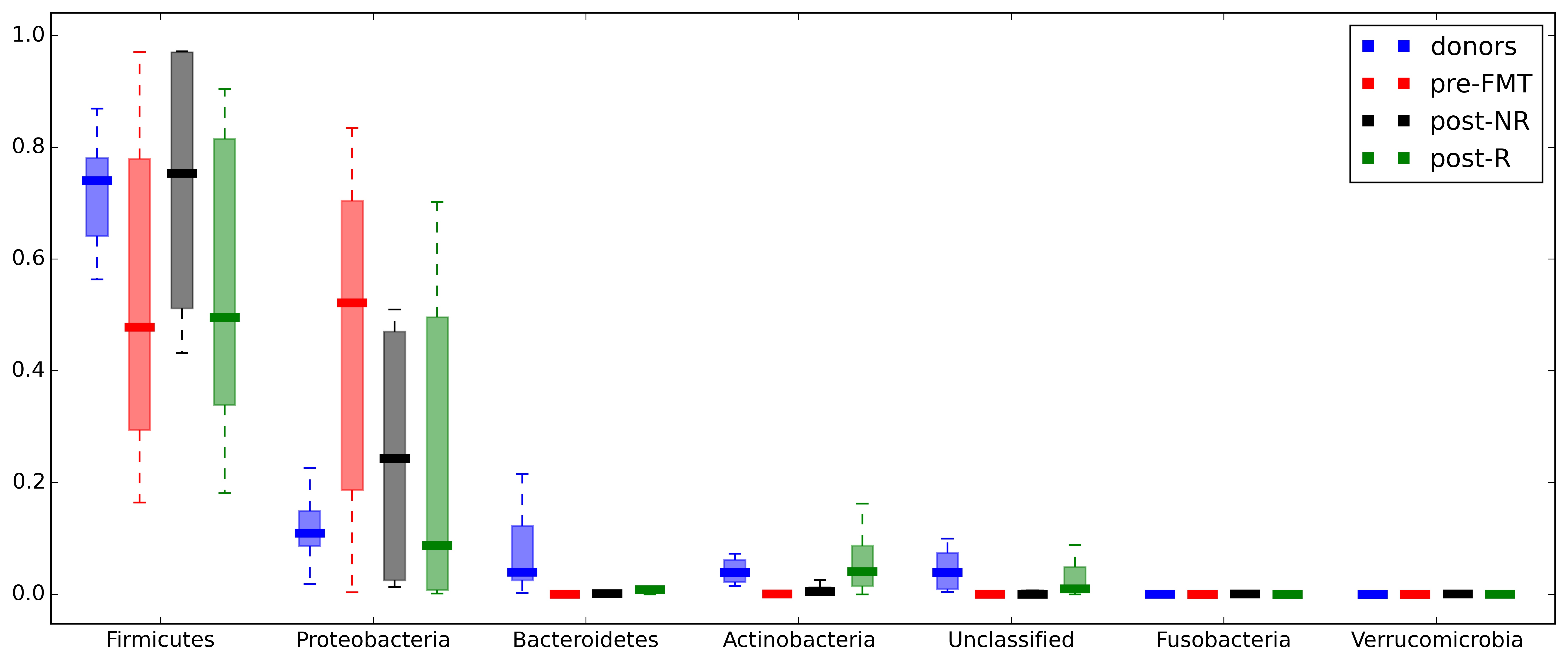
Due to the relatively small sample size, we formed a Healthy group comprising all samples from donors and post-FMT patients in resolution and a CDI group consisting of all samples from pre-FMT and post-FMT patients not in resolution. Inclusion of post-R samples in the Healthy group has the virtue of challenging the biomarkers $\beta$ and $\gamma_{t}$ to be sensitive to partial restoration to normal of the gut flora of recovering patients.

From the frequency data, we constructed $\beta$, as described in Section 5.3. Linear discriminant analysis yielded an axis in $\mathbb{R}^{7}$ along a direction determined by a unit vector whose loadings are specified in Table 1. The loadings revealed that $\beta$ captures a complex combination of the frequencies of the various phyla, with only Fusobacteria and Verrucomicrobia playing lesser roles due to their low frequencies.

Phylum	LDA loadings for $\beta$	LDA loadings for $\gamma_{t}$
Firmicutes	-0.412	-0.079
Proteobacteria	-0.644	0.059
Bacteroidetes	0.517	-0.623
Actinobacteria	0.267	-0.340
Unclassified	0.275	-0.443
Fusobacteria	-0.010	-0.119
Verrucomicrobia	0.006	-0.525

Table 1: Loadings of the directions that determine the axes in 7-D space for $\beta$ and $\gamma_{t}$.

Figure 7: Boxplot of the values of the diffusion Fréchet functions.

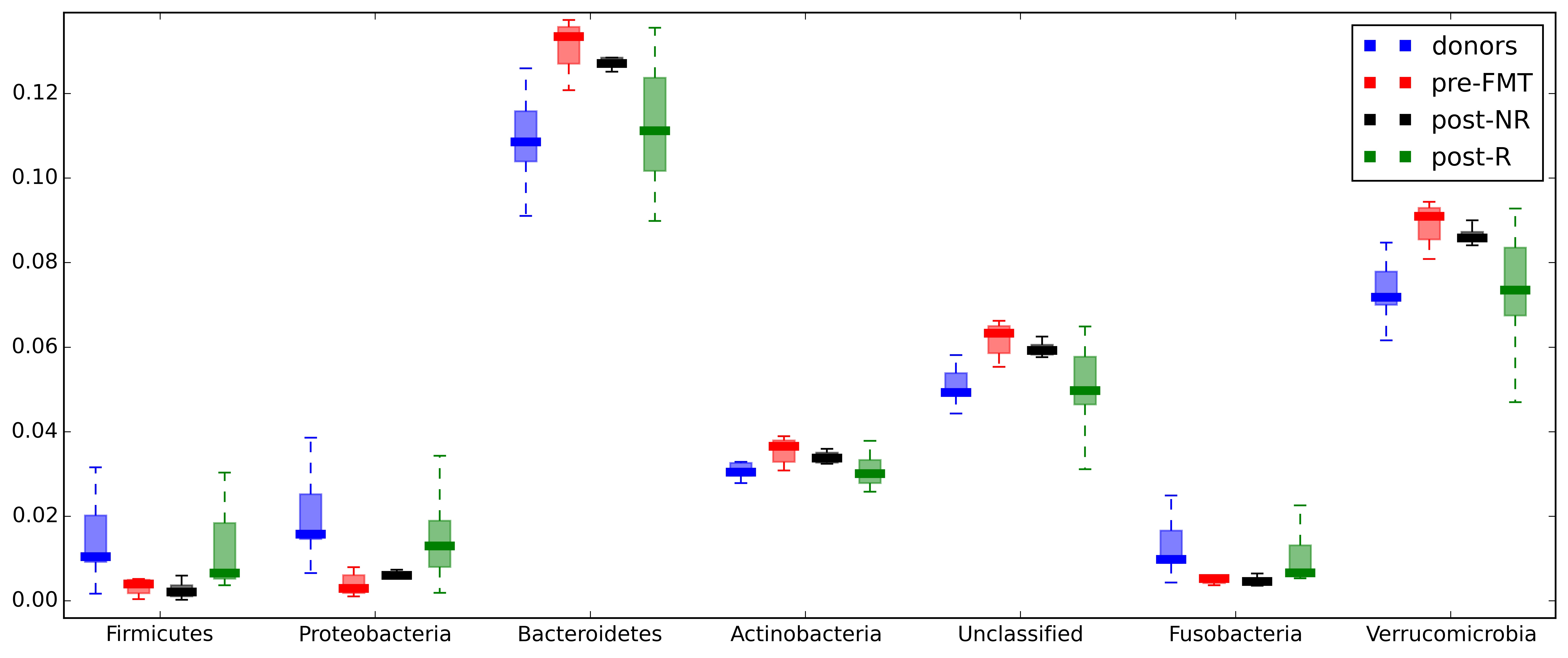
A similar analysis was carried out for $\gamma_{t}$. We tested a range of values for the significance level $\alpha$ used in network sparsification and the scale parameter $t$. The values $\alpha=0.1$ and $t=7.75$ were selected because they optimized the performance of $\gamma_{t}$ as measured by the area under its receiver operating characteristic (ROC) curve [20], a plot of the true positive rate (sensitivity) against the false positive rate (1 - specificity) at different threshold levels. Figure 7 shows boxplots of the values of the diffusion Fréchet function for the four groups. Table 1 shows the loadings for a unit vector in the direction of the axis in $\mathbb{R}^{7}$ space associated with $\gamma_{t}$ that indicate that the composition of the sub-communities associated with Bacteroidetes and Verrucomicrobia have a dominant role in characterizing CDI through $\gamma_{t}$, followed by Unclassified and Actinobacteria. Note that the model identifies Verrucomicrobia as a key player, whereas its contribution to $\beta$ is minor simply because its count is significantly smaller than the counts for other phyla.

Figure 8 provides a comparison of the ROC curves for $\beta$ and $\gamma_{t}$, $t=7.75$, demonstrating that $\gamma_{t}$ has a superior performance relative to $\beta$ in characterizing CDI and recovery from CDI.

Figure 8: ROC curves for $\beta$ (black) and $\gamma_{t}$ (blue), for $t=7.75$.

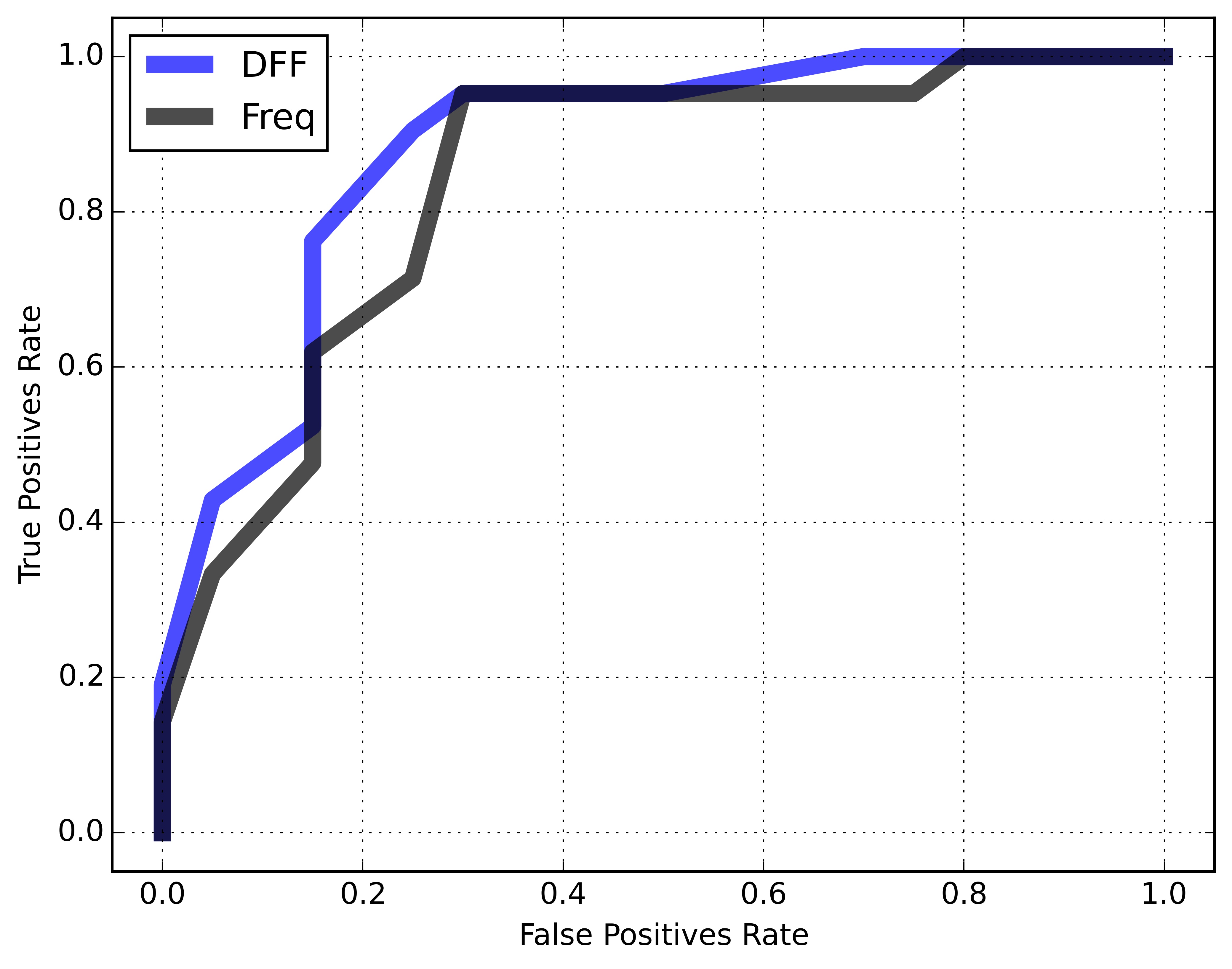
At the threshold value $a=-1.128$, $\gamma_{t}$ attained a true positive rate of $83\%$ and a false positive rate of $20\%$, as estimated from data for 20 healthy and 21 infected samples, respectively. At $a=-1.108$, the sensitivity increased to $91\%$ with a false positive rate of $25\%$. As samples from recovering CDI patients whose gut flora are only partially restored to normal have been included in the healthy group, we conclude that $\gamma_{t}$ also shows good sensitivity to the effects of FMT treatment. In this regard, we note that a significant portion of the false positives correspond to samples from post-FMT treatment patients in resolution whose gut flora are only partially restored to normal.

6 Concluding Remarks

We introduced diffusion Fréchet functions and diffusion Fréchet vectors for probability measures on Euclidean space and weighted networks that integrate geometric information at multiple spatial scales, yielding a pathway to the quantification of their shapes. We proved that these functional statistics are stable with respect to the Wasserstein distance, providing a theoretical basis for their use in data analysis. To demonstrate the usefulness of these concepts, we discussed examples using simulated data and applied DFVs to the analysis of data associated with fecal microbiota transplantation that has been used as an alternative to antibiotics in treatment of recurrent CDI. Among other things, the method provides a technique for detecting the presence and studying the organization of sub-communities at different scales. The approach enables us to address such problems as quantification of structural variation in bacterial communities associated with a cohort of individuals (for example, bacterial communities in the gut of multiple individuals), as well as associations between structural changes, health and disease.

Diffusion Fréchet functions may be defined in the broader framework of metric spaces equipped with a diffusion kernel. However, their stability in this general setting remains to be investigated. As remarked in Section 3, the present work suggests the development of refinements of diffusion Fréchet functions such as diffusion covariance tensor fields for Borel measures on Riemannian manifolds to make their geometric properties more readily accessible.

References

- [1] R. R. Coifman, S. Lafon, Diffusion maps, Applied and Computational Harmonic Analysis 21 (1) (2006) 5–30. doi:10.1016/j.acha.2006.04.006.
- [2] C. Villani, Optimal Transport, Old and New, Springer, 2009.
- [3] P. Chaudhuri, J. Marron, Scale space view of curve estimation, The Annals of Statistics 28 (2) (2000) 408–428.
- [4] U. von Luxburg, A tutorial on spectral clustering, Statistics and Computing 17 (4) (2007) 395–416. doi:10.1007/s11222-007-9033-z.
- [5] D. Díaz Martínez, F. Mémoli, W. Mio, Multiscale covariance fields, local scales, and shape transforms, in: F. Nielsen, F. Barbaresco (Eds.), Geometric Science of Information, Vol. 8085 of Lecture Notes in Computer Science, Springer, 2013, pp. 794–801.
- [6] D. Díaz Martínez, F. Mémoli, W. Mio, The shape of data and probability measures, arXiv preprint arXiv:1509.04632.
- [7] D. Lusseau, K. Schneider, O. J. Boisseau, P. Haase, E. Slooten, S. M. Dawson, The bottlenose dolphin community of Doubtful Sound features a large proportion of long-lasting associations, Behavioral Ecology and Sociobiology 54 (4) (2003) 396–405. doi:10.1007/s00265-003-0651-y.
- [8] L. Lovász, Random walks on graphs: A survey, Combinatorics, Paul Erdos is Eighty 2 (1996) 353–398.
- [9] C. P. Kelly, J. T. LaMont, Clostridium difficile more difficult than ever, New England Journal of Medicine 359 (18) (2008) 1932–1940. doi:10.1056/NEJMra0707500.
- [10] C. Vincent, D. A. Stephens, V. G. Loo, T. J. Edens, M. A. Behr, K. Dewar, A. R. Manges, Reductions in intestinal Clostridiales precede the development of nosocomial Clostridium difficile infection, Microbiome 1 (1) (2013) 18. doi:10.1186/2049-2618-1-18.
- [11] J. S. Bakken, T. Borody, L. J. Brandt, J. V. Brill, D. C. Demarco, M. A. Franzos, C. Kelly, A. Khoruts, T. Louie, L. P. Martinelli, et al., Treating Clostridium difficile infection with fecal microbiota transplantation, Clinical Gastroenterology and Hepatology 9 (12) (2011) 1044–1049. doi:10.1016/j.cgh.2011.08.014.
- [12] E. Gough, H. Shaikh, A. R. Manges, Systematic review of intestinal microbiota transplantation (fecal bacteriotherapy) for recurrent Clostridium difficile infection, Clinical Infectious Diseases 53 (10) (2011) 994–1002. doi:10.1093/cid/cir632.
- [13] D. Shahinas, M. Silverman, T. Sittler, C. Chiu, P. Kim, E. Allen-Vercoe, S. Weese, A. Wong, D. E. Low, D. R. Pillai, Toward an understanding of changes in diversity associated with fecal microbiome transplantation based on 16S rRNA gene deep sequencing, MBio 3 (5) (2012) e00338–12. doi:10.1128/mBio.00338-12.
- [14] A. M. Seekatz, J. Aas, C. E. Gessert, T. A. Rubin, D. M. Saman, J. S. Bakken, V. B. Young, Recovery of the gut microbiome following fecal microbiota transplantation, MBio 5 (3) (2014) e00893–14. doi:10.1128/mBio.00893-14.
- [15] C. Lee, J. Belanger, Z. Kassam, M. Smieja, D. Higgins, G. Broukhanski, P. Kim, The outcome and long-term follow-up of 94 patients with recurrent and refractory Clostridium difficile infection using single to multiple fecal microbiota transplantation via retention enema, European Journal of Clinical Microbiology & Infectious Diseases 33 (8) (2014) 1425–1428. doi:10.1007/s10096-014-2088-9.
- [16] S. Rush, S. Pinder, M. Costa, P. Kim, A microbiology primer for pyrosequencing, Quantitative Bio-Science 31 (2) (2012) 53–81.
- [17] B. H. Junker, F. Schreiber, Analysis of Biological Networks, Vol. 2, John Wiley & Sons, 2011.
- [18] N. J. Foti, J. M. Hughes, D. N. Rockmore, Nonparametric sparsification of complex multiscale networks, PloS One 6 (2) (2011) e16431. doi:10.1371/journal.pone.0016431.
- [19] D. A. Schult, P. Swart, Exploring network structure, dynamics, and function using NetworkX, in: Proceedings of the 7th Python in Science Conferences (SciPy 2008), Vol. 2008, 2008, pp. 11–16.
- [20] T. Fawcett, An introduction to ROC analysis, Pattern Recognition Letters 27 (8) (2006) 861–874. doi:10.1016/j.patrec.2005.10.010.