The Structure of the Circumgalactic Medium of Galaxies: Cool Accretion Inflow Around NGC 1097¹

Abstract

We present Hubble Space Telescope far-UV spectra of 4 QSOs whose sightlines pass through the halo of NGC 1097 at impact parameters of $\rho=48-165$ kpc. NGC 1097 is a nearby spiral galaxy that has undergone at least two minor merger events, but no apparent major mergers, and is relatively isolated with respect to other nearby bright galaxies. This makes NGC 1097 a good case study for exploring baryons in a paradigmatic bright-galaxy halo. Ly$\alpha$ absorption is detected along all sightlines and Si III $\lambda 1206$ is found along the 3 smallest $\rho$ sightlines; metal lines of C II, Si II and Si IV are only found with certainty towards the inner-most sightline. The kinematics of the absorption lines are best replicated by a model with a disk-like distribution of gas approximately planar to the observed 21 cm H I disk, that is rotating more slowly than the inner disk, and into which gas is infalling from the intergalactic medium. Some part of the absorption towards the inner-most sightline may arise either from a small-scale outflow, or from tidal debris associated with the minor merger that gives rise to the well known ‘dog-leg’ stellar stream that projects from NGC 1097. When compared to other studies, NGC 1097 appears to be a ‘typical’ absorber, although the large dispersion in absorption line column density and equivalent width in a single halo goes perhaps some way in explaining the wide range of these values seen in higher-$z$ studies.

1. INTRODUCTION

It is now thought that the circumgalactic medium (CGM) of a galaxy represents a genuine transition zone for the recycling of baryons. The term CGM refers to the gas that exists in some sense ‘outside’ of the interstellar medium (ISM) of a galaxy, yet ‘inside’ its virial radius, distinct from the surrounding intergalactic medium (IGM) (see, e.g. Shull, 2014). The idea of the CGM has replaced that of the classic “gaseous halo” or “galactic corona”, in large part because of a recognition of the many physical processes that probably compete to sustain it: baryons may be flowing out of galaxies as part of stellar or AGN winds (Rubin et al., 2014; Bordoloi et al., 2014a, and refs. therein), or from inflows from the IGM (Ford et al., 2014; Martin et al., 2012; Rubin et al., 2012), or from the interplay between merging galaxies, stripped via tidal interactions (e.g. Rupke & Veilleux, 2013; Bessiere et al., 2012); or they may simply be part of in-situ cloud formations that arise from thermal instabilities in a halo (Mo & Miralda-Escude, 1996; Hobbs et al., 2013, and refs. therein). These processes drive galactic evolution, so characterizing the CGM around galaxies is essential for understanding how galaxies evolve.

One way to study galaxy CGMs is through the absorption lines they cause in the spectra of background objects. The method of detecting QSO absorption line systems (QSOALSs) in background QSO spectra, and then searching for galaxies at the same redshift as the absorption, has been in practice for three decades. Since the launch of the Hubble Space Telescope (HST), QSOALSs have been found in the ultraviolet (UV) at very low redshifts; in particular, the installation of the Cosmic Origins Spectrograph (COS, Green et al., 2012) aboard HST has enabled the production of several extensive surveys that have targeted the CGMs of specific samples of relatively low-$z$ galaxies, including, for example, “COS-Halos” (Tumlinson et al., 2013; Werk et al., 2013), “COS-Dwarfs” (Bordoloi et al., 2014b), “COS-GASS” (Borthakur et al., 2015) as well as several unnamed surveys (e.g. Stocke et al., 2013; Borthakur et al., 2013; Burchett et al., 2015, 2016). If the goal of a study is to understand the nature of the CGM around galaxies as a function of their properties, then surveys that look for absorption lines from selected galaxies are perhaps the most valuable, because selecting galaxies prior to searching for any absorption reduces the bias in only finding CGMs around particular types of galaxies or in particular environments.

All these surveys study the statistical properties of absorbing clouds that arise from single sightlines through single galaxies. Conclusions are drawn about the CGMs of galaxies assuming that galaxies are sufficiently similar that probing many galaxies with single sightlines is the same as probing a single galaxy with many sightlines. Or at least — as larger samples of galaxy-absorber pairs have become available, and a more nuanced approach has been possible — that galaxies with similar characteristics (the same luminosity, halo mass, type, star-formation rates, etc.) will have similar enough CGMs that the properties of the absorbing clouds — if really linked to these properties — will become apparent.

Is it valid to assume that similar galaxies can have the same CGMs? Given two identical galaxies, can their properties dominate the state of the baryons within $R_{v}$ so directly that they end up having highly similar CGMs? Or are the processes that manufacture the CGM inherently too chaotic to lead to reproducible structures? Indeed, can QSOALSs provide any unique signature of a CGM’s origin at all?

One way to test these assumptions is to probe the CGM of individual galaxies along multiple sightlines. Absorption by the CGM of one galaxy should depend on far fewer variables in such experiments because, obviously, galaxy properties are fixed for a single galaxy. Such studies ought to be able to more easily expose which property of a galaxy a CGM most depends on.

There are several ways to probe galaxies along more than a single sightline. Multiple sightlines have been observed from either closely separated QSO sightlines (Bechtold et al., 1994; Fang et al., 1996; D’Odorico et al., 1998; Dinshaw et al., 1998, 1997) or lines of sight towards the multiple images of lensed QSOs (Petry et al., 1998; Smette et al., 1992; Monier et al., 1998; Rauch et al., 2001). In many cases, such investigations have focussed on determining the sizes of absorbing clouds when lines were detected (or not) in common along the sightlines, although the use of these background sources also provided examples of rarer Damped Ly$\alpha$ (DLA) systems (Cooke et al., 2010; Ellison et al., 2004; Churchill et al., 2003; Kobayashi et al., 2002; Lopez et al., 1999; Zuo et al., 1997; Smette et al., 1995), the detection of which might be expected for lensed QSOs when the lensing object is predicted to be relatively close to the sightlines. For these latter absorbers, multiple sightlines have now been used to provide evidence for changes in gas-phase metallicities on scales of a few kpc (Lopez et al., 2005).

For lensed QSOs, lensing galaxies have been at $z\gtrsim 1$, and the absorbing galaxy has been undetected (even if a lens redshift is inferred from the configuration of the lensed images), and the galaxy’s properties remain unknown. There are only a small number of examples where both multiple background sightlines have been observed at a high enough resolution to show absorption systems, and a galaxy has been confirmed spectroscopically to be at the same redshift as an absorber (Rauch et al., 2002; Rogerson & Hall, 2012; Chen et al., 2014; Muzahid, 2014; Zahedy et al., 2016). Explanations for the observed absorption have covered the entire gamut of CGM origins, from ancient, as well as recent, outflows, to tidal debris, inflowing streams and stripped gas. Even with these studies then, there is no clear agreement on a common origin for absorption from lensing galaxies.

An alternative method for studying multiple sightlines through a galaxy (and the one adopted in this paper) is to select nearby galaxies for study. Galaxies at very low-redshifts have large angular footprints on the sky, which make it easier to identify multiple QSO sightlines that pass through the galaxy at interesting impact parameters. The main disadvantage of working at low-redshifts is that most of the absorption lines of interest all lie in the UV, and can only be reached using HST. Not only is access to the satellite limited due to high demand, but the telescope’s modest mirror size restricts spectroscopic observations to only the brightest objects. Nevertheless, it was always expected prior to its launch that HST would probe galaxy halos along more than single sightlines (e.g. Monk et al., 1986) and indeed, some attempts were made with the first generation of the HST spectrographs (e.g. Norman et al., 1996; Bowen et al., 1997). Significant progress has been made in the last few years, however, as COS has enabled observations of the fainter QSOs that constitute a higher surface density on the sky.

Keeney et al. (2013) first made use of the enhanced throughput of COS by observing 3 QSO sightlines 74$-$172 kpc from the edge-on spiral ESO 157$-$49 at $cz=1673$ km s^-1; they detected absorption from Ly$\alpha$, and both low- and high-ion species, and suggested that some of the absorbing clouds are the remnants of recycled galactic fountain gas. Perhaps a more obvious set of galaxies to probe with multiple QSOs, however, might be M31 and M33. Being the closest bright galaxies to the Milky Way, they have very large angular diameters on the sky, and finding a high number of background probes at interesting impact parameters is straightforward. The problem with both these galaxies is that their velocities are low. Maps of 21 cm emission show that the high H I column density gas in the disk of M33 extends from $\sim-60$ to $-300$ km s^-1 (e.g. Putman et al., 2009), and from $\sim-50$ to $-600$ km s^-1 for M31 (e.g. Corbelli et al., 2010) (the latter having more than twice the angular diameter on the sky than M33). The complexity of the H I on the largest scales between M31, M33 and the Magellanic Stream and the difficulties in separating out Galactic, Local Group, and extragalactic H I can be seen in the maps of Braun & Thilker (2004). These low velocities make it difficult to separate any absorption from the galaxies with absorption from HVCs in the Milky Way, particularly Complexes H & G (e.g. Fig. 1 of Tripp & Song, 2012); they also make it impossible to observe any extragalactic Ly$\alpha$ absorption, which is lost in the saturated Ly$\alpha$ profile of the Galaxy. Nevertheless, attempts to utilize the many QSOs behind both galaxies have been made recently by Rao et al. (2013) and Lehner et al. (2014). We return to these studies later (see §8.1).

In this paper, we investigate absorption — including that of Ly$\alpha$ — by multiple QSO sightlines that pass through the halo of NGC 1097, a galaxy that lies well away from the Local Group. Our paper is divided into several sections. In §2 we summarise the properties of NGC 1097, its local environment, and the large scale structure (LSS) in which it is found. In §3 we briefly discuss some of the work that led to the selection of NGC 1097 and the background QSOs for study. In §4 we describe the HST observations and the reduction of the data, and in §5 we analyse in detail the characteristics of the absorption lines detected. §6 outlines the results of photoionization modelling of the results, although full details are presented in the Appendix. In the remaining sections we discuss the interpretation of our results. We consider possible configurations of the CGM of NGC 1097 based on the kinematics of the absorbing gas in §7, examine the statistical properties of the detected absorption in §8, and compare our results to other studies of absorbing galaxies in order to determine whether NGC 1097 is a ‘typical’ absorbing galaxy in comparison to the growing set of higher-$z$ absorbing galaxies (§8.1). We discuss our results in §9, where we suggest the most likely origin for the absorption (§9.1), and briefly compare our data with the results from numerical simulations (§9.2). We summarise our results in §10.

Throughout this paper we adopt the cosmology $H_{0}=73$ km s^-1 Mpc^-1, $\Omega_{m}=0.27$, and $\Omega_{\Lambda}=0.73$, when required.

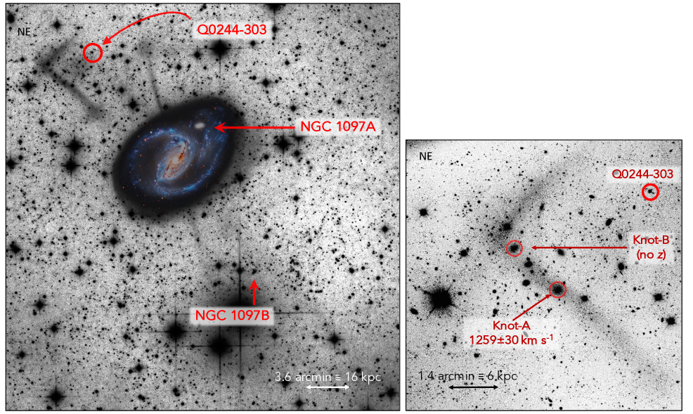
Figure 1.— The field of NGC 1097 ($cz=1270$ km s^-1), showing its stellar tidal streams. Left: Part of a multicolor (22 hr total) composite image of the galaxy taken with a Ceravolo 30 cm telescope and Apogee U16M camera by Rick Stevenson in Queensland, Australia in 2013. The two most prominent streams, towards the north-east, are easily seen: the well-known ‘dog-leg’ stream is to the left, with its right-angle kink, while the stream to the right appears to end in a bulbous cloud of stars. To the south-west, the left-most stream is fainter and shorter than the northern streams, but is clearly visible. The southern stream to the right is very faint ($\sim 27.6$ mag arcsec^-2) but may be the longest of the four, and perhaps wider and more amorphous than the other three streams. The streams themselves are likely the stellar remains of a low-mass galaxy that has passed through the disk of NGC 1097 (Higdon & Wallin, 2003; Amorisco et al., 2015). NGC 1097’s companion galaxies are also marked — NGC 1097A ($cz=1368$ km s^-1) and NGC 1097B (see Appendix B). The position of one of the QSOs discussed in this paper, Q0244$-$303, is marked, but the remaining sightlines are outside the field of view (see instead Fig. 3). Right: Portion of a 400 sec $V$-band FORS2 image extracted from the ESO Archive [originally published by Galianni et al. (2010)]. The dog-leg stellar trail is shown more clearly in relation to the position of Q0244$-$303, and the only part of the stream with a spectroscopic redshift, Knot-A, is indicated.

2. NGC 1097 and its Environment

2.1. Properties of NGC 1097

Table 1Parameters for NGC 1097

		Ref.
RA, Dec:	02:46:18.95, $-$30:16:28.8	1
Heliocentric velocity $v_{\odot}$:	1271$\pm 10$ km s-1	2
Hubble flow velocity:	1105$\pm 12$ km s-1	3
Inclination, PA of major-axis:	$40\pm 5$°, 130°	4
Mag $b_{J}$, $M(b_{J})$, $L$:	10.1, $-20.8$, $1.4\,L_{*}$	5
Diameter $D(0)_{25}(B)$:	9.55′ $\equiv 42$ kpc	6
H I massa:	$7.7\times 10^{9}M_{\odot}$	2
Star Formation Ratea:	$5\pm 1\>M_{\odot}$ yr-1	7
Stellar mass [$\log(M_{\odot})$]a:	$10.5\pm 0.1$	8
Total mass [$\log(M_{\odot})$]:	$\simeq 12.0\pm 0.2$	9
Adopted Distance $D$:	$15.1\pm 1.1$ Mpc	10
Virial Radius, $R_{\rm{vir}}$:	280 kpc	10

Note. — References: (1) Position of nucleus in HST WFPC2 F218W image from data in the Hubble Legacy Archive; (2) From 21 cm emission line data of Koribalski et al. (2004); (3) Heliocentric velocity converted to CMB velocity using the conversion given by the NED; (4) Higdon & Wallin (2003); (5) Doyle et al. (2005); (6) de Vaucouleurs et al. (1991) (RC3); (7) Calzetti et al. (2010); (8) Skibba et al. (2011); (9) Converted from stellar mass — see §2.1; (10) See §2.1.

NGC 1097 is an SB(s)b galaxy (Figs. 1) which hosts a Type 1 AGN that is surrounded by a $\sim 700$ pc ring of on-going star-formation (e.g. Barth et al., 1995; Prieto et al., 2005). A global systemic velocity for the galaxy can be taken from 21 cm emission line measurements, the two most pertinent H I maps having been made by Ondrechen et al. (1989) and Higdon & Wallin (2003). Ondrechen et al. cited a heliocentric systemic velocity of $v_{\odot}=1280\pm 10$ km s^-1, but Higdon & Wallin did not derive $v_{\odot}$ from their data. Since these maps were produced, the H I Parkes All-Sky Survey (HIPASS) single-dish survey Bright Galaxy Catalog has listed $v_{\odot}=1271\pm 3$ km s^-1 (Koribalski et al., 2004).

Converting the heliocentric systemic velocity to a Hubble flow distance is not necessarily correct, since corrections for local group motions, and motions of NGC 1097 towards the Fornax cluster (see §2.3) are not accounted for. The difference between $v_{\odot}$ and the CMB background is 166 km s^-1, giving a corrected velocity of $1105\pm 12$ km s^-1 if the HIPASS velocity is used, and a corresponding distance of $15.1\pm 1.1$ Mpc, which we adopt in this paper. This gives a scale of 4.4 kpc arcmin^-1 on the sky. This distance agrees well with a distance of $14.2\pm 2.4$ Mpc given by Tully et al. (2008) based on a distance modulus derived from the 21 cm line width-galaxy luminosity relationship of Tully & Fisher (1977). The apparent magnitude of NGC 1097 is $b_{J}=10.1$ (Doyle et al., 2005), which would translate to an absolute magnitude of $M_{*}(b_{J})=-20.8$ for $D=15.1$ Mpc. If an $L^{*}$ galaxy has an absolute magnitude of $M_{*}(b_{J})=-20.4$ (Norberg et al., 2002), then $L/L_{*}=1.4$ for NGC 1097.

We calculate the virial radius $R_{v}$ for NGC 1097 as follows. With the stellar mass of the galaxy known (Table 1), the DM mass can be calculated using the stellar-mass to halo-mass correlations given by Behroozi et al. (2013): for $\log M^{*}=10.5\pm 0.1$, $\log M_{h}(M_{\odot})=12.1$. The error in converting between stellar mass and halo mass is of the same order as the error in the stellar mass itself, $\sim 0.2$ dex. This halo mass is similar to $\log M_{h}(M_{\odot})=11.8$ found by Higdon & Wallin (2003) when fitting a simple disk+halo model to the observed 21 cm rotation curve. Using the approximations given by Maller & Bullock (2004), the virial halo radius is $R_{v}\simeq 280$ kpc. Deviations of order 0.2 dex in stellar mass would change this value by $\pm 40$ kpc, so the value of $R_{v}$ is not precisely known. The value of $R_{v}=280$ kpc agrees with the conversion between galaxy luminosity and $R_{v}$, $M_{h}$ given by Stocke et al. (2013, their Fig. 1), providing their halo abundance matching curves are used; their “adopted minimum $M/L$ ratio” gives an $R_{v}$ that is 30% smaller. For a halo with this mass, the corresponding virial velocity is 140 km s^-1, and the virial temperature is $6.9\times 10^{5}$ K.

These, and other relevant physical parameters of NGC 1097 (some of which are discussed later in this paper) are listed in Table 1.

2.2. Local Environment

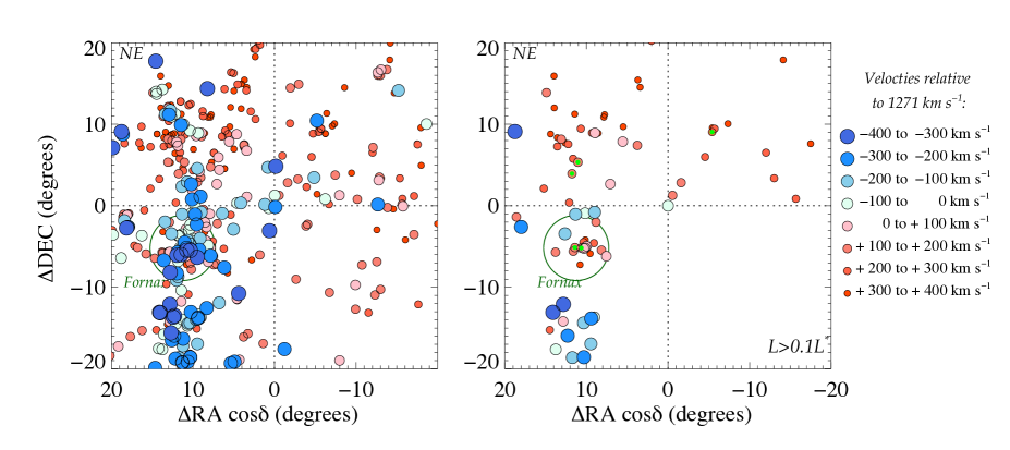
Figure 2.— Distribution of galaxies within $\pm 400$ km s^-1 of NGC 1097. The position of NGC 1097 is at the center of each plot (dotted lines). Left: All galaxies with redshifts cataloged by the NED are plotted. Galaxies which have redshifts greater than NGC 1097 are shown as small, red circles; those with redshifts less that NGC 1097 have larger, bluer circles. The magnitudes of the velocity differences, as a function of the color and size of the circles, are shown in the legend on the extreme right of the figure. The largest, bluest circles are for galaxies with the highest blueshifts relative to NGC 1097, while the smallest, reddest circles have the highest redshift relative to NGC 1097. Right: Same as left panel, but only galaxies with luminosities $\gtrsim 0.1L^{*}$ are plotted. The 5 red circles filled with green are the 5 closest galaxies with luminosities greater than 0.8 times that of NGC 1097, assuming that their radial redshifts really represent Hubble flow distances. The labelled (unfilled) green circle in each panel shows a 4 degree radius from the center of the Fornax cluster, which corresponds to $\approx 1.4$ Mpc at the distance of Fornax.

At the outskirts of the galaxy, NGC 1097 shows clear signs of minor merger events, one on-going, the other occurring in the more distant past. The most obvious feature is the presence of NGC 1097A (see Fig. 1), an elliptical galaxy which has a velocity of $1365\pm 45$ km s^-1, and which appears to be interacting with (and disrupting) the outer north-west spiral arm of the parent galaxy. The interaction produces two additional H I arms to the south of the galaxy, well beyond the optical disk (see Fig. 4b of Higdon & Wallin 2003, and the outer contour of the 21 cm emission outlined in Fig. 3). The galaxy has a magnitude of $m_{B(0)}=13.6$ or $M_{B}=-17.3$ at a distance of 15.1 Mpc, largely equivalent to the Large Magellanic Cloud (LMC) near our own Galaxy.

More uniquely, NGC 1097 also shows four optical filaments or streams (Wolstencroft & Zealey, 1975; Arp, 1976; Lorre, 1978). The structures show no optical, X-ray, or radio emission (Wehrle et al., 1997, and refs. therein). All four streams can be seen in the left panel of Figure 1. The filament oriented to the north-east is remarkable for showing an acute right-angle bend, producing an ’L-shaped’ structure which has become known as the ‘dog-leg’.

In discussing the possible origin of the streams, Higdon & Wallin (2003) suggested that they were caused by the minor merger of a low-mass dwarf disk galaxy, with the lack of any detectable H I and H II emission due to ram-pressure stripping of the dwarf’s gas by the disk of NGC 1097. Higdon & Wallin were able to show that X-shaped tidal streams — including features resembling the dog-leg seen towards NGC 1097 — could be reproduced in $N$-body simulations of a dwarf disk galaxy with a mass of only 0.1 % of the host galaxy mass (so in this case, $M_{*}\>\sim\>6\times 10^{8}\>M_{\odot}$) passing through a disk-dominated potential. The streams are, therefore, most likely the stellar remains of a disrupted galaxy, and are not caused by outflowing gas from the center of NGC 1097. More recently, Amorisco et al. (2015) modelled the streams using the infall of a disky dwarf galaxy that has passed its pericenter three times, and which has lost two dex in mass. They too were able to reproduce the right-angle kink seen in the dog-leg stream.

The interpretation that the streams are composed mainly of stars is consistent with spectra of two regions of the dog-leg obtained by Galianni et al. (2010). Within the dog-leg stream itself, there are several ‘knots’ of stars. The only feature with a confirmed redshift is Knot-A, which Galianni et al. measured to be $cz=1259\pm 30$ km s^-1, and which likely gives a redshift for the stream at that position (Fig. 1, right panel). Galianni et al also observed a second source near the right angle of the trail (their ’Knot-B’, see Fig. 1), but were unable to derive a redshift; for both sources, no emission lines were detected, as might be expected if the streams were actually hot outflows from the center of the galaxy. Moreover, the SEDs of the knots are inconsistent with thermal or synchrotron emission (Higdon & Wallin, 2003).

2.3. Global Environment

In order to examine how the CGM of NGC 1097 might be related to (and influenced by) the wider IGM, we would like to know the galactic structures in which the galaxy is found. To examine the relationship of NGC 1097 to its environment, we extracted all galaxies with known redshifts within $\pm 20$ degrees of the galaxy from the NASA/IPAC Extragalactic Database (NED). If we naively assume that the difference in velocity between the surrounding galaxies and NGC 1097 in the line-of-sight direction gives a distance of $\Delta v/H_{0}$, then the nearest galaxies that have luminosities $\geq 0.8$ times that of NGC 1097 lie $\sim 4-5$ Mpc away (NGC 908, 1371, 1399 and 1398, and 6dF J0342193$-$352334).

NED’s listing is not a magnitude-limited sample (there is currently no magnitude-limited survey covering this wide a field around NGC 1097) but the collation is useful in showing the proximity of NGC 1097 to the Fornax Cluster, which lies 12 degrees away. The galaxy surface density of Fornax reaches the background at only $\sim 6$ degrees (Ferguson & Sandage, 1989) from its center, which almost certainly places NGC 1097 outside of the cluster. The left-hand panel of Figure 2 shows a roughly linear distribution of galaxies running North-South on the sky, defining the filamentary structure containing Fornax cluster galaxies, and the color coding in the figure highlights the filament’s velocity gradient (Waugh et al., 2002). NGC 1097 appears to lie close to, but not obviously within, the filament; not only does its distance from the central concentration of galaxies suggest that it lies away from the filament, but its velocity is several hundred km s^-1 lower than the majority of the background galaxies in that direction. If the distance from us to the center of Fornax is $19-20$ Mpc (e.g. Madore et al., 1999; Dunn & Jerjen, 2006), then NGC 1097 is $\sim 5-6$ Mpc from its center.

The right-hand panel of Figure 2 shows the same distribution of galaxies, but only after selecting galaxies with $L>0.1L^{*}$. The magnitudes of galaxies listed by the NED are inhomogeneous in their filter selection, and the conversion of those magnitudes to a luminosity is approximate. The five closest galaxies mentioned above that have comparable luminosities to that of NGC 1097, are highlighted as circles with green centers, and are all over $4-5$ Mpc away. The panel demonstrates that there are far fewer bright galaxies near NGC 1097 than the left hand panel suggests, and that there are no companion galaxies to NGC 1097 with comparable luminosity. Figure 2 therefore suggests that NGC 1097 is a relatively isolated galaxy, probably lying at the edge of a large scale structure filament.

While it is possible that NGC 1097 may be moving towards the cluster, there is no evidence that it has experienced any recent tidal stripping from any intracluster medium. In this sense, the CGM of the galaxy has most recently been defined primarily by the local interactions discussed in the previous section.

3. QSO Target Selection

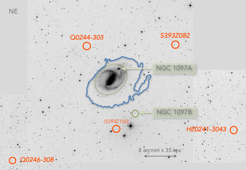
Figure 3.— Positions of QSO sightlines observed in this paper relative to NGC 1097. The image is constructed from portions of the STScI Digitized Sky Survey data, aligned with each other to reproduce the correct angular distances on the sky. QSOs observed in our COS program are labelled with circles; we also show the position of S394Z150 even though our COS data found it to be a white dwarf. The green dotted line around NGC 1097 marks its optical diameter $D(0)_{25}$, while the thick blue line shows the maximum extent of the galaxy detected by Higdon & Wallin (2003) at 21 cm, at a level of $\simeq 1.3\times 10^{19}$ cm^-2. If the virial radius $R_{v}$ of NGC 1097 is 280 kpc then the furthest sightline from the galaxy, towards HE 0241$-$3043, is at an impact parameter of $\simeq 0.6\>R_{v}$ in this figure.

Over the last few years we have been searching the fields of nearby galaxies to find those with multiple QSOs behind them. We began by compiling a list of the top 250 low-redshift galaxies with the largest angular diameters on the sky, and with velocities $\geq 700$ km s^-1 to ensure that Ly$\alpha$ absorption would be well away from the geocoronal Ly$\alpha$ emission line (see §4.1.1) in COS data. For each galaxy, we used available Galaxy Evolution Explorer (GALEX) satellite catalogs to collate all sources within 200 kpc, that had a measured Far-UV (FUV) flux greater than 40 $\mu$Jy [$F_{\lambda}=5\times 10^{-16}$ ergs cm^-2 s^-1 Å^-1, or $m$(FUV)=19.9]. An additional cut was made to remove objects with GALEX FUV widths greater than 15 arcsec FWHM, in order to avoid extended sources that would pass only a small fraction of their cataloged flux through the small COS aperture.

To corroborate which of the UV sources were extragalactic, and not Milky Way stars, the GALEX-generated lists of FUV-bright objects were cross-correlated with the latest release of the SDSS redshift catalogs, the NED, and the SIMBAD database. The galaxies were then ranked simply by the surface density of the background probes. NGC 1097 was one of a small number of galaxies that had more than $5$ sources satisfying the criteria described above and became one of the potential targets for HST follow-up.

Table 2Journal of Observations

									Impact Parameters
QSO	RA & DEC	Galactic	$B(J)$	FUV		Observation	Time	Observed	$\rho$	$\rho$	$\rho/$
name	(J2000.0)	$l$ & $b$	(mag)	($\mu$Jy)	$z_{\rm{em}}$	Date	(min)	Flux	$(^{\prime})$	(kpc)	$R_{v}$
Q0244$-$303	02:46:49.87,	226.573,	18.4	126	0.53	2013$-$08$-$09	204	1.14	11.0	48.2	0.17
	$-$30:07:41.3	$-$64.569
2dFGRS	02:45:00.77,	226.556,	19.1	57	0.34	2013$-$05$-$27	294	0.70	19.2	84.2	0.30
S393Z082	$-$30:07:22.4	$-$64.962
Q0246$-$308	02:48:22.00,	227.747,	17.3	97	1.09	2013$-$08$-$06	245	1.28	34.2	149.9	0.54
	$-$30:38:06.8	$-$64.238
HE0241$-$3043	02:43:37.66,	227.488,	17.2	155	0.67	2013$-$06$-$21	116	3.90	37.6	164.8	0.59
	$-$30:30:48.1	$-$65.259
2dFGRS	02:46:13.34	227.431	19.2	63	0.0	2012$-$10$-$17/20	308	1.0	13.3	…	…
S394Z150	$-$30:29:42.2	$-$64.700

In addition, NGC 1097 was observed as part of a GALEX Cycle 1 program that we designed to obtain FUV grism spectra of UV-bright objects in nearby galaxy fields. Unfortunately, we did not discover any new QSOs near NGC 1097, but did recover many of the objects already known. Further details on the original discoveries of the QSOs selected for our HST study are given in Appendix A along with notes on our GALEX grism spectra.

Table 2 lists the QSOs observed in this paper; in order to provide a more succinct nomenclature for the objects, we abbreviate the QSO names to the simpler forms of Q0244, S393Z082, Q0246 and HE0241 throughout the text. A fifth object, 2dFGRS S394Z150, believed to be an AGN at $z=0.131$, was observed as part of our program. Its identification proved to be incorrect, however — the object is likely a white dwarf star instead. Additional details are given in Appendix A, but this object is listed at the end of Table 2 as it was used in the analysis of the other spectra, discussed below.

4. COS Observations and Data Reduction

4.1. Co-addition of Sub-Exposures

Our GO program (12988) observations were made with COS using the G130M grating and the Primary Science Aperture (PSA). A journal of the observations is given in Table 2. Data were taken in TIME-TAG mode. Two different grating positions were used, centered at 1291 and 1327 Å, to provide (after coadding all the exposures) some data in the gap between the two segments of the photon-counting micro-channel plate detector (Holland et al., 2012). Each sightline was observed over $3-5$ orbits per visit, with all of the four available FP-POS offsets used to reduce fixed-pattern noise.

While the sub-exposures were wavelength calibrated by the pipeline, their wavelengths disagreed with each other in pixel-space, because of shifts in the dispersed light across the detector, caused by the difficulty of returning the grating to exactly the same position after any movement. In order to coadd spectra for a given sightline, we interpolated the flux arrays onto a common wavelength grid at a dispersion of 0.01 Å pix^-1, close to the initial value from the pipeline. To account for wavelength shifts in individual exposures that were not corrected for by the pipeline calibration, we compared positions of the strongest lines visible in each exposure, and measured the fractional pixel shifts needed to align the features. Any offsets found were added as zero-point shifts to the wavelength arrays.

To co-add data at wavelengths obtained by only some of the exposures, and to account for exposures with unequal exposure times, we calculated a weighted average from the COUNT-RATE arrays in the x1d files, with weights formed from the inverse of a spectrum’s variance. We propagated an error array $\sigma_{i}$ at each pixel $i$ from the gross counts $n$ of a spectrum using the lower Poisson confidence levels given by Gehrels (1986). Each error array was smoothed by a 10 pixel boxcar average to eliminate effects from fluctuations in individual pixels. The average count-rate of all the exposures was formed by weighting each sub-exposure by the inverse of the variance array.

The long and short segments were co-added using the same weighting scheme described above. The final spectrum for each sightline was rebinned by a factor of 3 to 0.03 Å pix^-1 ($\equiv 7$ km s^-1 pix^-1 at 1220 Å) to better sample the data given the resolution of COS. The final spectra had S/N ratios of $6-8$ per rebinned pixel at 1220 Å, and $8-10$ pix^-1 at 1340 Å.

4.1.1 Background Contribution from Ly$\alpha$ Airglow

Searching for Ly$\alpha$ absorption lines at the redshifts of nearby galaxies is hampered by two problems. First, at redshifts close to zero, Ly$\alpha$ lines are unobservable because the QSO flux is completely extinguished by the damped Ly$\alpha$ absorption from our own Milky Way. Second, geocoronal Ly$\alpha$ emission filling the 2.5 arcsec diameter circular COS PSA will contribute additional flux at the wavelengths of the expected extragalactic absorption. This would make lines seem weaker than they really are, and lead to an under-estimate of H I column densities. The Ly$\alpha$ airglow is distributed over a wide spectral range, and when observing objects with low count rates, the emission can be a significant additional background source near the rest wavelength of Ly$\alpha$.

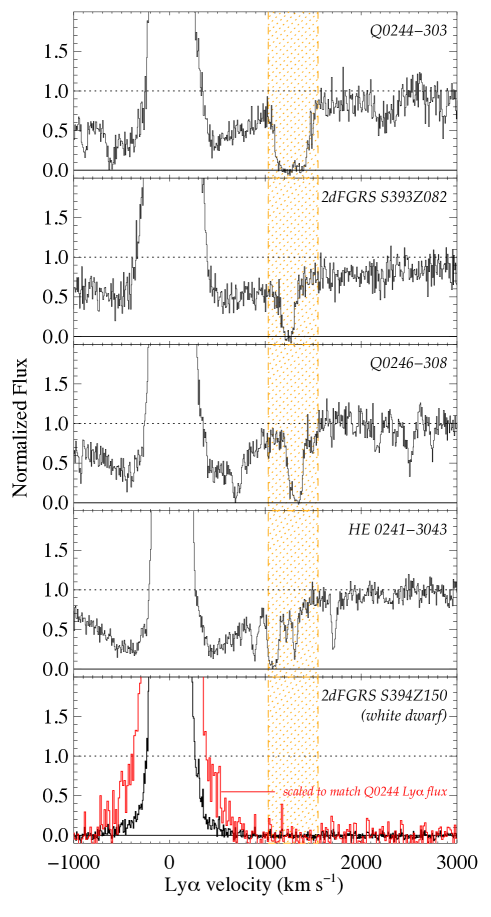
Figure 4.— The top 4 panels show COS spectra for the QSOs whose sightlines pass through the halo of NGC 1097. The orange dashed regions shows the approximate extent of Ly$\alpha$ absorption from NGC 1097. The bottom panel shows the spectrum of the WD star S394Z150 that was also observed in our program. The black line shows the measured normalized flux, while the red line shows the same flux (binned by a factor of 2 for clarity) scaled (by a factor of 5.6) such that the geocoronal Ly$\alpha$ emission line would have the same flux as the line seen in the spectrum of Q0244, which had the highest Ly$\alpha$ emission line flux of the 4 QSOs. This panel shows that at velocities similar to that of NGC 1097, emission from the wings of Ly$\alpha$ geocoronal emission add no additional background counts to the observed Ly$\alpha$ absorption lines seen from NGC 1097.

Portions of the co-added spectra near rest-frame Ly$\alpha$ are shown in Figure 4. At the lowest velocities, geocoronal Ly$\alpha$ emission dominates. The spectrum of Q0244 shows the widest Ly$\alpha$ absorption from NGC 1097 (the extent of which is indicated by orange lines), but there is no flux at the center of the absorption line profile, suggesting that at least by a redshift of $cz=1270$ km s^-1, Ly$\alpha$ airglow does not contribute to the spectrum’s flux. Additional information comes from the observation of the WD star, S394Z150, where Ly$\alpha$ absorption in the star’s atmosphere is so strong that there is no flux over a wavelength range much wider than that which is usually extinguished from interstellar Ly$\alpha$ in the Milky Way. The spectrum of the WD is shown in the bottom panel of Figure 4, where only geocoronal Ly$\alpha$ emission is left at the bottom of the damped Ly$\alpha$ trough (black line). In our sample, the strongest geocoronal Ly$\alpha$ was observed towards Q0244, and Figure 4 shows the extent of the emission towards the WD after the peak of the Ly$\alpha$ emission has been scaled to that of Q0244 (red line). The figure shows that by $\simeq 800$ km s^-1, any contribution from airglow is negligible and any Ly$\alpha$ absorption lines at those velocities would be unaffected.

4.1.2 Final Wavelength Accuracy

To provide a precise zero-point to the wavelength calibration, we tied the wavelengths of features in the COS data to the velocity of 21 cm emission measured towards the QSOs from H I profiles extracted from the Parkes Galactic All-Sky Survey (GASS) survey (McClure-Griffiths et al., 2009) . The median heliocentric velocities of the 21 cm H I emission along all four QSO sightlines were nearly identical, $+9$ km s^-1. We matched this velocity to those of the strongest low-ionization ISM lines seen in the COS spectra, which are expected to arise in the same gas detected at 21 cm, namely Si II $\lambda 1190,1193$, the S II $\lambda\lambda 1250,1253,1259$ triplet, Si II $\lambda 1260$ and C II $\lambda 1334$. In fact, the velocities of these lines did not all agree; in collating line centroids for all 4 sightlines, differences of $0-12$ km s^-1 ($\sim 0-2$ rebinned pixels) were found between the different ions. There are several possible reasons for this: line centers may be measured incorrectly because of low S/N in the line profile; weaker components of the strongest lines may have different profiles compared to weaker lines where such components are not detected; or errors may arise in the wavelength solution applied to the detectors, or to x-walk along the detector in regions where the gain-sag is high. Without knowing which of these effects dominate, we decided to match the 21cm emission velocity of +9 km s^-1 to the average velocity of all seven MW lines; as a consequence, between $1190-1334$ Å, the error in measuring the wavelength of any narrow feature ought to be $\sim\pm 6$ km s^-1 or about 1 rebinned pixel. This wavelength range covers all the lines we expected to see from NGC 1097, except the Si IV $\lambda\lambda 1393,1402$ doublet.

5. Results

5.1. Absorption Line Measurements

In the final co-added COS spectra we searched for absorption from NGC 1097 from a variety of species, which are listed in Tables 3$-$6. In this section, we describe the analysis of detected absorption lines, while in §5.2 we discuss how limits to column densities were derived when no absorption was detected. Much of this analysis follows the methods described by Bowen et al. (2008). In particular, the way in which the data were normalized, the procedures used to measure velocities $v$, column densities $N$, and Doppler parameters $b$, of the absorbing gas by generating theoretical Voigt line profiles and fitting these to the data, and the use of Monte Carlo (MC) simulations to account for errors in the fits arising from Poisson statistics, were identical to those described by Bowen et al. (2008), and are not repeated here.

The results of the line profile fits are given in Tables 3$-$6. For all the fits performed, $b$ and $N$ were allowed to vary as free parameters. In all cases, however, $v$ was fixed to the values shown in column 2. The alignment of components between metal lines and Ly$\alpha$ is discussed in detail below for each sightline. Values of $\sigma(b)_{T}$ and $\sigma(N)_{T}$ are given in these tables (columns 7 & 9): these represent the errors in $b$ and $N$ resulting from a combination of continuum fitting errors and theoretical line profile fitting errors (again, see Bowen et al., 2008). The errors in velocity (column 4) are simply those found from the MC simulations, and do not include possible systematic errors discussed in §4.1.2.

For multicomponent fits, the total (summed) column density over all components is given at the bottom of column 8 for each species. The error on this total, given at the bottom of column 9 for each species, was calculated from the distribution of summed column densities derived for each MC run (and not from any combination of the errors from individual components, because these are not independent for multicomponent fits).

Tables 3$-$6 also include the equivalent widths (EWs) $W$ of detected lines (or upper limits when no lines were detected—see below). Several of the absorption lines from NGC 1097 were blended with other higher redshift lines, in which case their EWs were derived directly from their theoretical line profiles and not measured from the data. The EWs of the individual components are given in column 5 of the tables, but when more than 1 component exists, the total EW in column 5 (referred to in column 1 as “total [p]”) is given for the EW of the blended components, which need not equal the sum of the individual component EWs.

Unfortunately, the resulting errors in $W$ for EWs that rely on the profile fits cannot be made using the errors in $N$ and $b$ because they are correlated in such a way that $N$ and $b$ can vary while $W$ stays the same. Instead, total EWs were recorded for each of the 300 MC profile fits, and used to form a distribution of EWs. The distributions of $W$ were always normally distributed, yielding an error $\sigma(W)$. Again, $W$ was measured for three possible continuum fits, yielding errors that were added in quadrature with $\sigma(W)$ to give a total error. These are the errors that accompany the EW totals in column 5.

Tables 3$-$6 also list total EWs measured in the traditional way, directly from the spectra, calculated over a specific number of pixels (referred to as “total [$N=$]” in column 1). The values of $N$ here are chosen simply to be large enough to cover all the detected components. These EWs are independent of the assumed LSF or any other assumptions about how the absorption line profile should be modelled. The errors listed include errors from Poisson noise and deviations from the continuum fitting, analogous to the column density errors described above.

5.2. Equivalent Width Limits and Column Density Limits for Undetected Metal Lines

In many cases, no metal lines were detected towards the QSO sightlines, and column density limits had to be derived from EW limits. Traditionally, the EW limit at some wavelength is taken to be $\sigma^{2}(W)=\sum^{N}_{i}\>(\sigma_{i}\>\delta\lambda)^{2}$, where $\delta\lambda$ is the wavelength dispersion in Å pixel^-1 and $N$ is the number of pixels that the sum is made over, centered at the wavelength of interest. Or more simply, if $\sigma_{i}$ is close to being the same value $\sigma$ over $N$ pixels (because the errors change slowly with wavelength) then $\sigma(W)=\sigma\delta\lambda\sqrt{N}$. The COS LSF consists of a Gaussian core superimposed on much broader wings, as a result of mid-frequency wavelength errors in the HST mirrors (Kriss, 2011; Holland et al., 2012). If the LSFs generated for the profile fitting described above are integrated, then 95.5% of the area of a line is enclosed in 14 of our re-binned pixels. We adopted $N=14$ as the value over which to measure EW limits, knowing that the most a line EW might be under-estimated would be by $\simeq 5$ %.

For undetected lines in the QSO spectra, we list upper limits of $2\sigma(W)$ in Tables 3$-$6. To derive column density limits we used $b$ values from other lines where possible, and the values adopted are listed in parentheses in column 6 of Tables 3$-$6.

In the following sections, we look in detail at the absorption lines detected along each sightline, and discuss the measurements made from the line profiles.

5.3. Absorption Lines Towards Q0244$-$303

5.3.1 Metal Lines

The absorption lines seen towards Q0244 are shown in Figure 5. Metal lines are detected towards Q0244 at at least two velocities; in the first case, C II $\lambda 1334$, Si II $\lambda 1193$, Si II $\lambda 1260$ Si III $\lambda 1206$ and Si IV $\lambda 1393$ are found at a velocity of 1384 km s^-1. This component is labelled A3 in Table 3, and categorizes the strongest metal-line absorbers along the sightline. There is also a marginal detection of Si II $\lambda 1190$ at this velocity, although its reality is based largely on the presence of the other Si II lines since its strength is below our detection threshold. As expected therefore, the weakest line of the four Si II lines, Si II $\lambda 1304$, is absent. Si IV $\lambda 1403$ at 1384 km s^-1 is contaminated by an O VI $\lambda 1032$ line at $z=0.35818$, from a system which also shows corresponding Ly$\beta$, Ly$\gamma$, Ly$\delta$ and O VI $\lambda 1037$. Hence the $\lambda 1403$ line is not used in the derivation of the Si IV column densities.

A second component is detected from Si III $\lambda 1206$ at 1227 km s^-1; although there are no other metal lines to confirm the reality of this component, there is clear evidence of Ly$\alpha$ at a similar velocity (see below), and so we consider this component to be real. This component is labelled A1.

Finally, a weak feature is detected near the C II $\lambda 1334$ A3 component, which, if a lower velocity C II absorption feature, would be at $v=1261$ km s^-1. This velocity is clearly different from that of A1 and A3. We label this possible system A2 in Table 3 and discuss its reality below.

In order to establish the velocity of components A1 & A3, all the metal lines were fit simultaneously. Fits were first made without including the Ly$\alpha$ line. (The Ly$\alpha$ components are clearly blended, so there is little information in the line profile to help establish the components’ velocities). Values of $b$ and $N$ were allowed to vary independently for each component of each species, and while $v$ was also allowed to vary, it was constrained to be the same for each component of each ion.

Although A2 is defined only by the possible existence of a weak C II line, Table 3 lists EW limits and column density limits for the other species at the same velocity. For Si III, a limit is hard to define, since any absorption would be blended with the A1 component. The Si III A1 component is broad, and the low S/N of the data makes the profile appear coarse, but there is no obvious need to add an additional component to represent possible absorption at the A2 velocity. We estimate a plausible column density for Si III based on adding a fictitious A2 (unresolved) component and seeing how the blended profile changes with $N$(Si III).

A similar problem exists for defining a C II column density limit for A1, since any line at that velocity would be blended with the defining A2 C II component. We again estimate an upper limit to C II at A1 by blending a hypothetical component (this time with the $b$ value of the broad Si III component) with the existing C II component.

Figure 5.— Absorption lines found towards Q0244. The Ly$\alpha$ line is contaminated by two other lines, O VI $\lambda 1031$ at $z=0.18272$ and H I $\lambda 930$ at $z=0.31229$; the expected profiles of these two lines are shown as dotted lines, although the data shown are already corrected for them (see text). As discussed in the text, only two components (A1 and A3) are fitted to the body of the Ly$\alpha$ line, but the position of a possible component seen in C II $\lambda 1334$ is labelled (A2).

5.3.2 Ly$\alpha$

The Ly$\alpha$ absorption lines detected from NCC 1097 are complicated by contamination by lines from two higher-redshift systems. One contaminant is Ly$\lambda 930$ arising from a system at $z=0.31229$; the H I from this system is very well constrained however, since Ly$\beta$, Ly$\gamma$, Ly$\delta$, Ly$\epsilon$, Ly$\lambda 923$ and Ly$\lambda 920$ lines are all present. Absorption can be fit with a single component to give $\log N$(H I)$\>=\>15.88$ and $b\>=\>38.9$ km s^-1. With these values we can calculate a profile for Ly$\lambda 930$ (shown as a dashed line in Fig. 5) and remove it from the data. There also likely exists a second contaminent to the Ly$\alpha$ complex, an O VI $\lambda 1031$ line at $z\>=\>0.18272$. This system is defined primarily by Ly$\alpha$, Ly$\beta$ and Ly$\gamma$ lines, and so appears secure. There is a feature at 1227.2 Å which is probably the O VI $\lambda 1037$ line from this system. The O VI absorption is weak and simple, and a fit to the O VI $\lambda 1037$ line gives $\log N$(O VI)$\>=\>14.19$, $b\>=\>20.6$ km s^-1. We again model the corresponding O VI $\lambda 1031$ line using these values and remove it from the Ly$\alpha$ lines from NGC 1097. Both these interloping Ly$\lambda 930$ and O VI $\lambda 1031$ lines are relatively weak compared to the strong Ly$\alpha$ lines from NGC 1097 and contribute little to the total EW.

The Ly$\alpha$ profile clearly argues for at least 2 components, but determining the column density for A3 remains problematic; without including any more information from the metal lines (apart from their velocity) values of $\log N$(H I)$=15.07$ and $b=18.9$ are obtained (Table 3), but the solution is not unique, and the same profile can be obtained for higher $N$(H I) and smaller $b$ values. An upper limit for these can be set by the appearance of damping wings, which is not seen in the data, and which occurs when $\log N$(H I)$\>\gtrsim 17.1$ and $b\lesssim 11$ km s^-1.

While a 2 component fit can adequately represent the observed Ly$\alpha$ absorption, we noted in the previous section the possible presence of an additional C II component — A2 — which could have a corresponding Ly$\alpha$ component. There is no information in the Ly$\alpha$ profile to constrain the physical parameters of a component matching A2, but we can explore how badly the Ly$\alpha$ $b$-values and column densities of A1 and A3 might be affected by including A2. An upper limit to $N$(H I) for A2 can be set at $\log N$(H I)$\>\simeq 18.1$, when the damping wings of A2 are wider than the entire profile. The maximum $b$-value of A2 is given by the $b$-value of the C II component, which has $b=10.9$ km s^-1. If $b$(C II) was defined purely by turbulent processes, then $b$(Ly$\alpha$) would be the same as $b$(C II), or 10.9 km s^-1. If $b$(C II) was entirely a thermal width, then the corresponding temperature would be $\sim 8.6\times 10^{4}$ K. The width of a Ly$\alpha$ line at that temperature would be $b$(Ly$\alpha$)$\>=38$ km s^-1. We can therefore use $b=10.9$ and $b=38$ km s^-1 as a lower and upper limit to $b$ for A2. We can then fix the velocity of all 3 components to those of the metal lines, vary $N$(H I) for A2 in fixed intervals, and then refit, to see how $N$(H I) and $b$ change for A1 and A3.

In fact, for either value of $b$ for A2, the values of $b$ and $N$(H I) change little for A1 and A3 until the $N$(H I) of A2 reaches its upper limit of $\log N$(H I)$\simeq 18.1$. For $N$(H I) less than this, most of the optical depth at the velocity of A2 is always taken up by A1, so increasing $N$(H I) for A2 makes little difference to the optical depth at the velocity of A2. This suggests that $N$(H I) for A1 and A3 may not be too badly affected by the presence of even a moderately strong Ly$\alpha$ component at the velocity of A2.

Finally, we note the presence of additional weak, higher velocity components, which we label A4 & A5 in Table 3 and Figure 5. The figure shows the Ly$\alpha$ profile after the contaminating O VI $\lambda 1032$ and H I $\lambda$ 930 lines have been divided out of the data. We find values of $N$ and $b$ from the profile fitting, but the lines are unresolved. The limit of the COS resolution is $\sim 15$ km s^-1 FHWM (ignoring the non-Gaussian shape of the LSF) or $b\lesssim 9$ km s^-1. The EWs of both Ly$\alpha$ lines lie on the linear part of the Curve of Growth so long as $b\gtrsim 7$ km s^-1, (i.e. $T\simeq 3,000$ K) with $\log N$(H I)$\>\simeq 13.1$. If $b$ is really less than 7 km s^-1, however, then $N$(H I) is a lower limit. As $b$ is unconstrained, we give $N$(H I) as a lower limit in Table 3.

It is useful to summarise the above discussion in terms of the total $N$(H I) along the sightline, a value we will use later in this paper. The lower limit to $N$(H I) is set by A1, and is $\log N$(H I)$\>\simeq 15.6$ (Table 3). The upper limit is set by a lack of a damping wing on the red-side of A3, $\log N$(H I)$\>\lesssim 17.1$; however, the possible existence of H I corresponding to the C II component A2 increases this limit to $\log N$(H I)$\>\lesssim 18.1$, at which point damping wings would be seen on both sides of the complex.

5.4. Absorption Lines Towards 2dFGRS S393Z082

5.4.1 Metal Lines

As shown in Figure 6, Si III $\lambda 1206$ is detected unambiguously at 1240 km s^-1 towards S393Z082, a system we label B1. A weak feature is also detected at the wavelength where C II $\lambda 1334$ is expected at the same velocity as B1, but the line could be O VI $\lambda 1032$ at $z=0.29863$, because there is also a very weak feature which could be Ly$\beta$ at that redshift. The corresponding O VI $\lambda 1037$ line is not detected at this redshift, but given the weakness of the $\lambda 1032$ line, this is not unexpected for unsaturated lines. Fitting Voigt profiles to the Ly$\beta$, O VI $\lambda 1032$ and (to provide an upper limit) O VI $\lambda 1037$, a solution of $b=13.8$ km s^-1, $\log N$(H I)$\>=\>13.7$ and $\log N$(O VI)$\>=\>13.5$ can be found (Fig. 7). Although an O VI/H I absorber with such a narrow line width is relatively rare, Tripp et al. (2008) have found such systems. Further, the ratio of the column densities in our fit, $\log$[$N$(H I)/$N$(O VI)]$=-0.17$ is consistent with the values found by Tripp et al. for the value of $\log N$(H I)$=13.7$ that we find for the system. Given the precise alignment of the two lines, and the plausibility of physical parameters obtained from the profile fits when compared to other O VI systems, we cannot be sure that the line at 1340.1 Å is C II from NGC 1097 and refrain from using it in our analysis. We note that if the identification is wrong, and the line is indeed C II $\lambda 1334$, then the profile fit to the line requires $\log N$(C II)$\>\simeq\>14.0$.

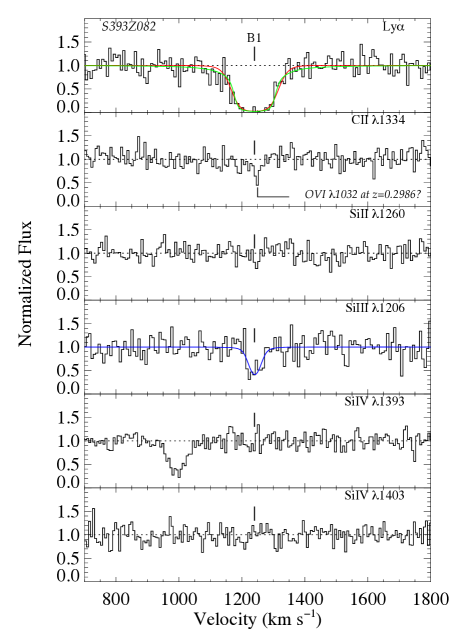
Figure 6.— Absorption lines found towards S393Z082. The values of $N$(H I) and $b$ are ill-constrained for Ly$\alpha$ absorption from NGC 1097: two theoretical line profiles are shown in the top panel, each representing nearly identical best-fits to the data: one has a high-$N$(H I)/low-$b$ solution (green), the other has low-$N$(H I)/high-$b$ values (red). The two profiles are nearly indistinguishable from each other. There exists a possible detection of C II $\lambda 1334$ (second panel), but the line is likely to be O VI $\lambda 1032$ at z=0.2986. Si III $\lambda 1206$ is the only metal line unambiguously detected from NGC1097 (fourth panel).

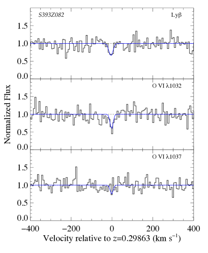
Figure 7.— While the line at 1340.1 Å towards S393Z082 could be C II $\lambda 1334$ absorption from NGC 1097 (see second panel of Fig. 6) another possible interpretation of this line, along with another at 1332.0 Å, is that they represent O VI $\lambda 1032$ and Ly$\beta$ absorption at $z=0.29863$ instead. This figure shows these lines (as well as the expected absorption from O VI $\lambda 1037$) in that rest-frame, as well as theoretical profile fits for $b=13.8$ km s^-1, $\log N$(H I)$\>=\>13.7$ and $\log N$(O VI)$\>=\>13.5$.

5.4.2 Ly$\alpha$

This is the simplest of the Ly$\alpha$ absorption lines associated with NGC 1097, but the physical parameters are not well constrained. The data have the lowest S/N of the 4 sightlines, and there is some ambiguity over the number of components to fit. A single component, which we label B1 in Figure 6, appears to be adequate; there is a slightly lower ‘shelf’ at 1100 km s^-1, and adding a component to match this feature changes $N$(H I) for B1 by a factor of 4. The MC simulations used to calculate the errors in $N$(H I) and $b$-values, however, suggest that the small amount of extra depth may well just be from noise, since in many cases, the feature is not replicated in the synthetic spectra. We therefore assume that no additional absorption occurs at this lower velocity.

The Ly$\alpha$ line provides an example of the classic problem of measuring $N$(H I) and $b$ when its EW lies on the flat part of the Curve of Growth. The line-profile fitting settles on two possible solutions, one with $b\>=\>46$ km s^-1 and $\log N$(H I)$\>=\>14.8$, and a second one with $b\>=\>19$ km s^-1 and $\log N$(H I)$\>=\>17.6$. The problem is exacerbated by the low S/N of the data providing insufficient constraints on the shape of the wings of the line. An analysis in which the width of the line is determined by a $b_{\rm{therm}}$ and a $b_{\rm{turb}}$ component (see Appendix C) shows that the change in $\log N$(H I) from 14.8 to 17.6 occurs when $T>1\times 10^{4}$ K. Figure 6 better shows the problem, where theoretical lines profiles for both the high-$N$ fit (green) and the low-$N$ fit (red) are drawn; the profiles for the two solutions are almost identical.

5.5. Absorption Lines Towards Q0246$-$308

5.5.1 Metal Lines

Along this sightline, Si III appears to be detected at the redshift of NGC 1097, and being shortward of Ly$\alpha$, the reliability of its identification is strong. This component is labelled C2 in Table 5 and Figure 8. There is an additional weak Si III component to the blue of C2, which is designated as C1.

Any C II $\lambda 1334$ from system C1 is lost in a line that, given its strength and width, is probably Ly$\alpha$ at $z=0.10224$ (Fig. 8, second panel) although there are no other corroborating lines. C II from system C2 is expected at 1340.5 Å, and a weak feature is seen very close to that wavelength, although it is nestled next to the high-$z$ Ly$\alpha$ line. $N$(C II) for the line is given in Table 5, and while we consider the detection to be real, it remains possible that the feature is simply an additional higher velocity ($z=0.10272$) component that is part of the strong high-$z$ Ly$\alpha$ line.

A feature is also seen at 1244.32 Å which could be N V $\lambda 1238$ from NGC 1097, but there is no N V $\lambda 1242$ line to confirm this. Fitting the N V $\lambda 1238$ line gives $\log N$(N V)$\>=\>13.50$ and $b=20$ km s^-1; with these values, the N V $\lambda 1242$ line should be detected, but is not. We therefore list only upper limits in Table 5.

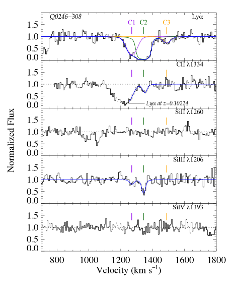
Figure 8.— Metal absorption lines found towards Q0246. The defining component of the system is labelled C2, seen in both Si III, Ly$\alpha$, and possibly, C II; weaker Si III and Ly$\alpha$ components exist at a more negative velocity, labelled C1. No Si II or Si IV is detected from either C1 or C2. C3 is identified only by Ly$\alpha$ absorption. The absorption at the expected velocities of the C II components is complex, and the strongest feature is probably a Ly$\alpha$ line at $z=0.10224$. Although we identify C II from system C2, it remains possible that this feature is part of that higher-$z$ complex at $z=0.10272$.

5.5.2 Ly$\alpha$

The Ly$\alpha$ absorption from NGC 1097 towards Q0246 is comprised of 3 components. Two of these well match the systems C1 & C2 identified in the metals; a third broader line is evident at a higher velocity, which we label C3 in Figure 8, but which has no corresponding metal-line absorption. The Ly$\alpha$ component in system C2 is another example of a saturated Ly$\alpha$, and constraining $N$(H I) is challenging. For this spectrum, the S/N is higher than for S393Z082, which helps constrain the fits of theoretical Voigt profiles; nevertheless, there is still a large uncertainty in $N$(H I) which is reflected in the errors listed in Table 5.

5.6. Absorption Lines Towards HE0241$-$3043

5.6.1 Metal Lines

No metal line absorption is detected from NGC 1097 along this sightline. The lack of detections are shown in Figure 9, and upper limits are listed in Table 6. Absorption by Si IV $\lambda 1393$ from NGC 1097 would be blended with a pair of Ly$\epsilon$ lines at $z\simeq 0.493$, so column density limits are measured for Si IV $\lambda 1403$ instead.

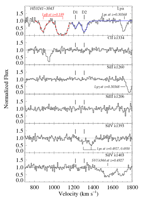
Figure 9.— Absorption lines found towards HE0241. Only Ly$\alpha$ is detected from NGC 1097.

5.6.2 Ly$\alpha$

Though no metal-lines are detected, two Ly$\alpha$ components are seen from NGC 1097. These are labelled D1 & D2 in Figure 9 and Table 6, and lie close to Ly$\beta$ lines from a two component complex at $z=0.18868$ & $z=0.18945$. D1 Ly$\alpha$ from NGC 1097 is slightly blended with the higher-$z$ of these two Ly$\beta$ lines, as can be seen in the figure. Unfortunately, any Ly$\alpha$ components at velocities less than that of D1 will be lost in the Ly$\beta$ lines. Neither D1 or D2 can, instead, be additional Ly$\beta$ components at $z\simeq 0.189$ because the corresponding Ly$\alpha$ lines are not seen at longer wavelengths. We can find no other systems for which D1 and D2 might be metal lines.

6. Photo-ionization models of absorbing clouds

In order to better understand the physical characteristics of the absorbing clouds, we have attempted to reproduce the measured values of, or limits to, the column densities for all ion species along the QSO sightlines using photoionization models. The results depend on various assumptions, and as the list is rather extensive, we present the details of our analysis in Appendix C. Unsurprisingly, only components with detected metal lines, those labelled above as A1, A3, B1, & C2 give useful constraints. In summary, the metallicities are probably sub-solar, $Z<0.3\>Z_{\odot}$ for A1, B1 & C2. For A3, however, we can find no single-phase solution, meaning that either the gas is not simply photoionized (or indeed collisionally ionized, which was also considered) or that the component-fitting model used to model $N$(H I) is inadequate.

7. Constraints on Halo Gas Kinematics

In this section we use the kinematics of the absorption lines toward NGC 1097 — the profiles of the lines and velocity centroids — to model the gas in the halo of the galaxy. We focus specifically on the detected Ly$\alpha$ lines as the H I absorbing gas is the most sensitive tracer of cool gas available from our observations, and is detected along all sight lines.

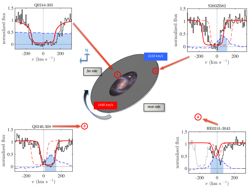
Figure 10.— Predictions of Ly$\alpha$ line profiles (red lines) for QSO sightlines passing through a rotating geometrically thin disk model, compared to our COS data. The center figure is a simple schematic of the galaxy-QSO configurations, with a disk that has approximately the same inclination and PA as NGC 1097 shown in Fig. 3; the SW side of disk is assumed to be closer to us, with the spiral arms trailing the rotation. The positions of the QSOs are indicated by red circles; they are arranged to roughly match their true configuration (Fig. 3), and indicate which structures of the model are intercepted along a given sightline. (The inset image of the image of the galaxy is not to scale, but is included to show the orientation of the spiral arms relative to the rotation.) The predicted line profiles are built from a model that follows the galaxy parameters in Table 1, as well as the positions of the QSOs on the sky, precisely. The disk has rotation speed of $v_{\rm{rot}}=+70$ km s^-1 and a turbulent velocity of 20 km s^-1. The model is qualitatively consistent with the data towards Q0244 and Q0246, although only one broad component is predicted for Q0244 when there are clearly two in the data; the model also over-predicts the strength of the absorption towards S393Z082, and cannot reproduce the double line profile towards HE0241. Also shown are $f_{\rm{min}}$ curves (blue dashed-line histograms) that are used to estimate the allowed rotation speed interval for each sightline (as shown by the blue shaded regions). For comparison, profiles are also plotted (red dashed lines) for an absorbing disk counter-rotating with respect to NGC 1097. Such counter-rotation would produce absorption at velocities quite different from that observed towards S393Z082 and Q0246.

7.1. Disk Models

Simulations of galaxy structures in a $\Lambda$CDM universe predict that the halos of galaxies should accrete gas from the IGM along cool gas streams that possess their own angular momentum (Danovich et al., 2015; Cen, 2014; Stewart et al., 2013). This leads us to question whether the absorption seen towards NGC 1097 might trace similar structures. We consider two variations of gas rotation in NGC 1097: a) a rotating disk model, and b) a rotating-inflow disk model, where gas is flowing into the disk (akin to an accretion disk). For reasons that we explain, we will also consider a third option, that of the same rotating-inflowing disk model, but with a conic outflow launched from the center of the galaxy, perpendicular to the disk. For all these models, we use the galaxy parameters listed in Table 1.

7.1.1 Rotating Disk Models

In this model, we assume an inclined thin disk rotating at a fixed azimuthal speed $v_{\rm{rot}}$. A positive value of $v_{\rm{rot}}$ indicates clockwise rotation of the disk shown in Figure 3 — the analysis by Quillen et al. (1995) suggests that the south-west (SW) side of the galaxy lies nearer to us than the north-east (NE) side, and therefore that the galaxy rotates with its spiral arms trailing the rotation. The column density of the disk is assumed to follow an exponential decline with the de-projected (e.g. Williams & Hodge, 2001) radius $\tilde{\rho}\propto\exp(-\tilde{\rho}/\tilde{\rho}_{d})$, where the disk scale is $\tilde{\rho}_{d}=11$ kpc. To model the absorption we assume that micro-turbulence in the gas produces lines with widths of $v_{\rm{turb}}=20$ km s^-1, which result in the observed line profiles after convolution with the COS LSF.

Our aim is to use the parameters described to predict the line profiles that would be expected along the four QSO sightlines. As there are many parameters that can be varied to produce the predicted profiles, we refrain from, e.g., attempting to minimize a $\chi^{2}$ statistic between the theoretical profiles and the data — there is no unique solution for the number of parameters available. Instead, we look for more qualitative agreements that might guide us toward finding a correct scenario for the origin of the absorption.

So, for example, by adopting of value of $v_{\rm{rot}}\simeq+70$ km s^-1, we find that our predicted profiles show some agreement with the observed data. (This velocity is smaller than the circular speed of the inner disk observed from 21 cm emission measurements, which is $\sim 200-300$ km s^-1, a point we return to in the next section.) Figure 10 shows the predicted profiles in comparison to the observed profiles. While the impact parameters of the two outer sightlines differ by only 15 kpc, the Ly$\alpha$ line profiles of each are markedly different, with the sightline towards HE0241 showing none of the saturated absorption seen towards Q0246. As the former sightline lies closer to the minor axis of the disk, a lower opacity would indeed be expected. Further, the absorption velocities towards Q0244 and HE0241 are centered around the systemic velocity of NGC 1097, as would be expected for sightlines at opposite ends of the galaxy’s minor axis.

In contrast, the sightlines towards S393Z082 and Q0246 lie close to the opposite ends of the major axis and the absorption ought to be shifted away from the galaxy’s systemic velocity, and with the velocities in opposite directions. The implied sense of rotation is consistent with that assumed for the inner disk; for comparison, Figure 10 also shows the results from a disk model where the gas counter-rotates with the galaxy ($v_{\rm{rot}}=-70$ km s^-1): here the predicted absorption clearly fails to match the data. As expected, the discrepancies are largest towards the sightlines along the major axis where differences in $v_{\rm{rot}}$ would be most noticeable.

To estimate the uncertainties associated with $v_{\rm{rot}}$, we define a minimum fraction of the observed line profile which lies on either side of the centroid velocity of the predicted absorption $v_{c}$, i.e. $f_{\rm{min}}(v_{\rm{rot}})={\rm{min}}[{\rm{EW}}(v>v_{c}(v_{\rm{rot}})),{\rm{EW}}(v<v_{c}(v_{\rm{rot}}))]/$EW. Hence a model whose predicted velocity is centered around the observed absorption would have $f_{\rm{min}}\simeq 0.5$. For predicted line profiles whose $v_{c}$ significantly deviates from the observed centroid velocity, $f_{\rm{min}}\ll 1$. To estimate the uncertainty of $v_{\rm{rot}}$, we calculate $f_{\rm{min}}$ for a range of $v_{\rm{rot}}$ values, and take the profile to be an acceptable replica of the data if $f_{\rm{min}}>0.2$. This variation of $f_{\rm{min}}$ as a function of $v_{\rm{rot}}$ is shown as a dashed line at the bottom of each panel in Figure 10. As noted above, some sightlines are more sensitive of the disk dynamics than others, depending on where they probe the disk. For example, the sightline towards Q0244 is largely insensitive to disk rotation (top left panel of Fig. 10), because its sightline passes close to the minor axis of NGC 1097, and hence $f_{\rm{min}}$ changes little for any value of $v_{\rm{rot}}$ ($f_{\rm{min}}\simeq 0.5$ for $-500$ km s^-1$<v_{\rm{rot}}<500$ km s^-1). The other sightlines provide more stringent constraints on $v_{\rm{rot}}$, as Figure 10 shows, and the similarity in the velocities at which $f_{\rm{min}}$ peaks in the three other panels, $\sim 70$ km s^-1, suggests that this is a good estimate of $v_{\rm{rot}}$.

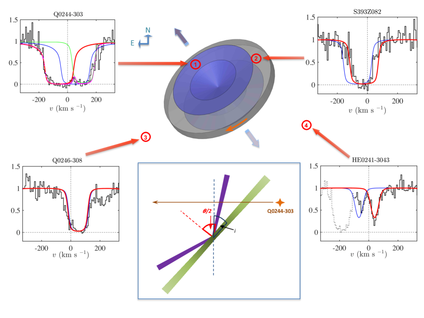
Figure 11.— Predicted Ly$\alpha$ line profiles (red lines) for QSO sightlines passing through gas accreting onto NGC 1097 via a rotating geometrically thin disk model, as compared to our COS data. The disk has $v_{\rm{turb}}=20$ km s^-1, a rotation speed of $v_{\rm{rot}}=70$ km s^-1, and an inflow speed along the disk’s (inward) radial direction of $v_{r}=70$ km s^-1. For comparison, the predicted line profiles for gas flowing away from the disk at a speed of $v_{r}=70$ km s^-1 are shown as blue lines. Compared to the thin-disk model shown in Figure 10, this model better reproduces the absorption seen towards S393Z082 and Q0246, component A1 towards Q0244, and D2 towards HE0241. However, it fails to account for components A3 towards Q0244 and D1 from HE0241. One way to explain component A3 towards Q0244 is to add a conic outflow (purple cone in the middle schematic) with an outflow velocity of 300 km s^-1 subtending an angular range of $65\arcdeg<\theta<70\arcdeg$ and extending out to at least 50 kpc above the disk. Such a model leads to the green line in the top-left panel, with the blend of the profiles from the two models shown in magenta. The inset diagram (middle, framed bottom panel) represents a cut through the model at the position of Q0244, that shows further how positive velocity absorption (i.e. component A3) can be obtained from a wide conic outflow (purple regions) as it emerges from the (green) disk. So long as $\theta\geq 90-i$, the edge of the outflow will have a velocity greater than the systemic velocity. In this particular scenario, outflowing gas occurs on only one side of the galaxy.

Although this model reproduces some of the absorption line features, there are notable discrepancies between the rotating disk model and the data. For example, the model fails to predict the two-component absorption seen towards HE0241. This might be the easiest discrepancy to understand. One possibility is that a thin disk model might no longer apply at such large radii. In fact, at a radius of $\sim 200$ kpc, the dynamical time $\sim 2\pi\tilde{\rho}/v_{\rm{rot}}$ is comparable to the Hubble time. Alternatively, the two-component absorption may mean that at large radii, H I clouds no longer form a homogeneous thin disk. Additionally, discrepancies associated with under- and over-prediction of the opacity along particular sightlines can be resolved if either $v_{\rm{turb}}$ or the column density profile deviate with radius (see, e.g., the variations in the rotation curves around a mean value in Ondrechen et al., 1989; Hsieh et al., 2011). More worryingly, the model predicts only one absorption component towards Q0244, whereas at least two are observed; and the absorption towards S393Z082 is somewhat narrower than the model predicts.

7.1.2 Rotating-Inflowing Disk Models with a Conic Outflow

As noted above, the rotation speed of an extended disk with $v_{\rm{rot}}\simeq 70$ km s^-1 is significantly smaller than the $200-300$ km s^-1 rotation speed of the inner disk (Ondrechen et al., 1989, see also §9.1). This fact, combined with results from $\Lambda CDM$ models that imply the existence of cold-flow accretion, lead us to consider a model in which the absorbing gas has an inward radial velocity $v_{r}$.

The results of such a model are shown in Figure 11; data towards sightlines that lie in the direction of the minor axis are more sensitive to $v_{r}$, and imply $v_{r}<100$ km s^-1. We find that a model with $v_{\rm{rot}}\simeq v_{r}\simeq 70$ km s^-1 improves the match between data and model towards some of the sightlines. Towards Q0244, the blue component, A1 is better reproduced by the model, but at the expense of A3, which is not predicted at all. The predicted absorption towards S393Z082 is improved, while the predicted absorption towards Q0246 is unchanged. One of the components towards HE0241, D2, now matches the predictions, but the other component, D1, is still not reproduced.

The values of $v_{\rm{rot}}$ and $v_{r}$ are not entirely unique and similar (but not superior) fits can be obtained for other $v_{\rm{rot}}$ and $v_{r}$ combinations. This model offers an improvement over the simple rotating disk presented above, but still fails to match all the observed features.

NGC 1097 shows moderate amounts of star formation at its center (Calzetti et al., 2010; Hsieh et al., 2011) so it is reasonable to consider the possible effects of an outflow in our models. In several studies where outflows have been traced by gas and dust emission (most notably towards AGN) a hollow cone geometry has been inferred whose axis lies along the disk’s angular momentum vector (Veilleux et al., 2001, 2005) and where the wind may be detected in emission out to several kpc above the disk, and potentially out to even larger scales in absorption (Murray et al., 2011).

We consider the effect of adding a hollow-cone model to our rotating-inflowing model by including gas that flows out of the galaxy along radial trajectories at a speed $v_{\rm{rad}}$. This addition is also shown in Figure 11. The most notable result from adding an outflow component is that we can replicate the additional A3 absorption component (Table 3) towards Q0244, using a model that has a cone with $v_{\rm{rad}}\simeq 300$ km s^-1 and that is so wide — $65\arcdeg<\theta<70\arcdeg$ — that part of the cone wall is still receding from us, providing an absorption component that has a positive velocity (redshift) with respect to the rest of the galaxy. This scheme is highlighted in the inset diagram in Figure 11. Wide angle outflow cones have been seen in the inner regions of some galaxies, e.g., towards ESO 097-G013 (Greenhill et al., 2003), so a weak outflow that contributes to the absorption is plausible. A wide, amorphous outflow more like the superwind seen towards M82 might be the best analog (e.g. Leroy et al., 2015, and refs. therein).

7.1.3 Contributions from Warped Disks

Galaxy disks are known to exhibit warps, especially in systems undergoing interactions with other galaxies. If the inclination angle of the disk changes with radius, for example, and/or the position angle of the major axis changes with radius, absorption line profiles could be replicated to better match the data with these added variables. For example, the simplest case is where the inclination angle varies with radius, which would allow for a wider range of $v_{\rm{rot}}$ at different radii. Among the various possibilities for geometrically thin disks we mention only two: good agreement between data and line profiles can be found when the outer disk has $v_{\rm{rot}}=250$ km s^-1 and $i=10\arcdeg$ (i.e. nearly face-on), or, $v_{\rm{rot}}=60$ km s^-1, $i=75\arcdeg$, and a very large disk scale of $\sim 30$ kpc. So, given the inclination of NGC 1097 ($40\pm 5\arcdeg$), substantial warping would be required to account for the observed absorption. There is some indication from the 21 cm H I maps of Higdon & Wallin (2003) that the outer spiral arms of NGC 1097 are disturbed by tidal interactions (which we discuss later), so distortions in the structure of any extended disk are a possibility. However, far more additional data on the nature of the warps in NGC 1097’s disk would be needed before they could be reliably added to our model.

7.2. Outflow Models

While a conic outflow can be added to the disk model to explain the additional absorption (component A3) seen towards Q0244, its inclusion is somewhat ad hoc, and leads us to examine whether, in fact, outflow models alone — with no contribution from an absorbing disk of gas — could adequately reproduce the observations. We assume bi-conic outflows whose symmetry axis is parallel to the angular momentum vector of the inner disk. Geometrically, the outflow is defined by an inner and an outer polar angle, as well as an inner and outer radius. This parameterization allows us to construct both spherical and polar outflows. By specifying an inner and outer radius to the outflow, intermittent flows or shells — rather than continuous winds — can also be modeled. We set the outer radius to arbitrarily large values; whether outflowing gas ejected from the center of a galaxy can travel well into, and survive within, the outer regions of a galactic halo, is a separate issue, and beyond the scope of this paper. For the sake of brevity, we do not reproduce a figure similar to Figures 10 and 11, but simply describe the results from our analysis.

We assume that the outflows are coasting at a constant radial outflow velocity, $v_{\rm rad}$. If mass is conserved along outflow lines (e.g., no mass loading), then the gas density is $n\propto r^{-2}$, where $r$ is the radial coordinate. For continuous spherical winds, this also implies that the absorbing column density declines as $1/\rho$. In contrast, for thin shell geometries whose size is larger than the impact parameter range in question, the column density is independent of $\rho$. Clearly, significant deviations from the above scalings could occur if $v_{\rm rad}$ varies with $r$, or if there are multiple ionization phases within the outflow (Rupke & Veilleux, 2013; Scannapieco & Brüggen, 2015). Such models cannot be constrained by the current data set.

7.2.1 Spherical Outflow Models

By virtue of isotropy, the absorption line profiles predicted from a spherical outflow model are centered symmetrically around the systemic velocity. For example, expanding shells would generally produce two-component line profiles as the sightlines towards the background QSOs intercept the front and back sides of the outflow. This well matches the double component profile (D1 and D2) towards HE0241, and we used these components to calibrate a thin-shell model with $\delta r\ll r$ (a similar approach was adopted by Tripp et al., 2011). Specifically, by matching the model to the D1 and D2 components, we find that the mass in the outflowing shell is $>3\times 10^{5}\eta\,{M_{\odot}}$, where $1/\eta$ is the mass fraction of the gas in the form of H I, a potentially small number related to the uncertainties in the ionization corrections and/or the multiphase nature of the outflow. The mass-loss rate is then of order $4\pi r^{2}\eta N({\rm H~{}I})m_{p}(v_{\rm rad}/r)\simeq 10^{-4}\eta(r/200\>{\rm kpc})(N({\rm H~{}I})/10^{14}\,{\rm cm}^{-2})(v_{\rm rad}/40\,{\rm km~{}s^{-1}})\,{M_{\odot}~{}{\rm{yr}}^{-1}}$, which is probably much smaller than the current rate of star-formation. Irrespective of this argument, thin-shell models fail to explain the decreasing gas opacity with impact parameter — the predicted column densities are always too low to produce the strong absorption seen along all the sightlines. Moreover, the asymmetric absorption around the systemic velocity along sightlines at opposite ends of the disk’s major axis (i.e. towards S393Z082 and Q0246) cannot be reproduced.

We find that the simplest models of spherical outflows seem to be inadequate for reproducing the observed absorption, and given the limited set of observational constraints, a more detailed analysis seems unwarranted.

7.2.2 Polar Outflow Models

In §7.1.2 we showed how adding a polar outflow to the rotating disk models could account for the A3 component seen towards Q0244. In general, however, models which include only polar outflows and no disk component run into difficulties explaining the absorption along the sightlines which lie in the direction of the major axis and are at large impact parameters, unless the opening angle is large or the flow extends far enough above the disk. For example, assuming an outflow that extends out to $R_{v}$, and opening angle of $>50\arcdeg$ is needed to produce absorption towards Q0246.

The model shown in Figure 11 assumes outflow from only one side of the galaxy, but a bipolar outflow would produce additional positive velocity absorption. Outflowing gas from the backside of the galaxy would need to extend further than the front-side flow to intercept the sightline. We do indeed see weak components — A4 and A5 — at higher velocities, which might fit such a scenario. Whether the extent and covering factor of the outer regions of an outflow could account for such weak absorption is unclear.

We should note that gas outflowing at the observed velocities would need to travel over timescales that are comparable to the dynamical time of the halo, which would most likely invalidate the simple conic geometry. For example, gas may be dragged perpendicular to the outflow if the halo is rotating, or minor mergers may disrupt the geometry of the escaping gas. Again, modelling the absorbing properties of such disrupted outflows is beyond the scope of this paper.

8. Global Properties of the absorption

We have observed 4 QSOs with impact parameters of $\rho=48-165$ kpc from NGC 1097 and searched for absorption from the galaxy along each sightline. The lowest quality spectrum has a 2$\sigma$ equivalent width limit of 35 mÅ at short wavelengths, defining the limiting EW of our survey for Ly$\alpha$ and Si III $\lambda 1206$. These limits correspond to column densities of $\log N$(H I)$\>=12.9$ and $\log N$(Si III)$\>=12.3$ (for Doppler parameters of $b\geq 7.1$ km s^-1, or thermal temperatures $\geq 3000$ K). We have seen that while the EWs of all the detected lines are measured precisely, $N$(H I) derived from the Ly$\alpha$ lines for 3 of the sightlines are less well defined, because the lines have equivalent widths where $b$ and $N$(H I) are degenerate. For the four sightlines, our most basic statistic suggests that the covering fraction of H I and Si III is 100 % and 75%, respectively, at a limit of $\rho=165$ kpc.

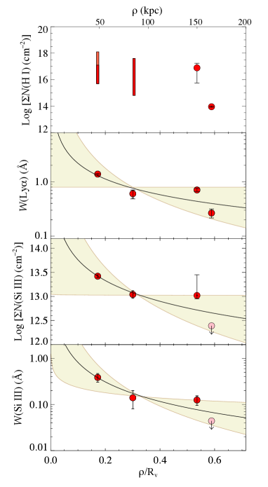
Figure 12.— Left: Distribution of total $N$(H I) summed over all components (top panel), Ly$\alpha$ EW (second panel), total $N$(Si III) (third panel), and Si III $\lambda 1206$ EW (bottom panel) towards NGC 1097 as a function of impact parameter normalized by virial radius. Our data are shown as red circles for detections, and pink circles for upper limits. For the $N$(H I) values in the top panel, our measurements are uncertain for the sightlines with the two smallest $\rho$, and we represent the range in possible $N$(H I) as two red/orange vertical bars. For Q0244, there are two possible upper limits to $N$(H I), one set by the maximum possible from component A3, which is shown in red, and one set by the maximum towards A2, extended in orange (§5.3). For S393Z082, the range is set by the two possible values of $N$(H I) that arise from two line profiles that are nearly identical (§5.4). For the three lower panels, power-law fits to the 4 points are shown as black lines, and the beige regions indicate errors obtained from $\chi^{2}$ confidence intervals (see text). Right: Contour plots of $\chi^{2}$ centered on the minimum values (shown with crosses) found for power-law fits to Ly$\alpha$ EWs (top panel), Si III EWs (middle panel) and $N$(Si III) (bottom panel). The best fit values are listed in the top right corner of each panel. Sets of $\alpha$ and $W^{*}$ or $N^{*}$ at the extreme deviations of the $1\sigma$ confidence intervals (black circles) are also indicated, and these two sets of values are the ones used to draw the shaded beige regions in the left-hand side of the plot.

The values of Ly$\alpha$ and Si III EWs, and H I and Si III column densities, plotted against their impact parameters normalized by the virial radius $R_{v}$, are shown in the left-hand column of Figure 12. The gas in the halo of the galaxy does not appear to be smoothly distributed. While a rank correlation test suggests that $\rho/R_{v}$ and $W$(Ly$\alpha$) are significantly anti-correlated, a Pearson’s product-moment analysis shows that the correlation is not significant (the probability of the null hypothesis is $p=0.18$, well above the 0.05 significance level often used to define a significant correlation). The same test for $W$(Si III) with $\rho/R_{v}$ actually finds more significance for anti-correlation.

Irrespective of these rank correlation tests, however, we would like to measure how $\rho/R_{v}$ and $W$(Ly$\alpha$) vary if the underlying relationship is a power-law, in part because a such a relationship is often suggested for higher-$z$ collations between EW and impact parameter in single-galaxy/single-QSO-sightline systems (see §8.1). Even though we have only 4 sightlines through NGC 1097, the sampling of multiple points in a single galactic halo is unique, and we therefore examine the results of fitting a power-law to the NGC 1097 data.

Both EWs and column densities are assumed to be related as

$$W=W^{*}\left(\frac{\rho}{R_{v}}\right)^{\alpha},\>\>N=N^{*}\left(\frac{\rho}{R_{v}}\right)^{\alpha}.$$ (1)

We fit the Ly$\alpha$ and Si III EWs, and the distribution of Si III column densities; we do not fit the H I column densities because we only have a range of values for 2 sightlines. We also take the Si III EW and column density upper limit towards HE0241 to be a detected value.

If a power-law fit to the data is justified, then the distributions do not vary smoothly with $\rho/R_{v}$. We can fit a power-law by varying $W^{*}$ or $N^{*}$, and $\alpha$, and minimizing the $\chi^{2}$ statistic between the NGC 1097 data and values expected from equation 1, but the reduced $\chi^{2}$ is $\chi^{2}_{\nu}\gg 1$ given the small errors relative to the overall dispersion in $N$ and $W$. To account for this, we introduce an additional “error” which accounts for the clumpiness in the distribution. This approach is the same as that used to account for patchiness in absorption from O VI in the Milky Way described by Bowen et al. (2008) [after the work of Savage et al. (1990)]. For each value of $W$ measured towards the QSOs behind NGC 1097 we introduce an additional relative error of $\sigma_{\rm{CL}}$ beyond that of the equivalent width error $\sigma(W)$ described in §5.2:

$$\sigma^{2}(W)_{T}=\sigma^{2}(W)+\sigma^{2}_{\rm{CL}}.$$ (2)

For the given points, $\sigma_{\rm{CL}}$ can be varied until $\chi^{2}_{\nu}=1$. The values of $\sigma_{\rm{CL}}$ that we find are listed in the right hand panels of Figure 12; for both the Ly$\alpha$ and Si III EW, $\sigma_{\rm{CL}}$ is similar, around 0.2 dex (top two panels), which might be expected if the Ly$\alpha$ and Si III absorbing regions are the same. For $N$(Si III), $\sigma_{\rm{CL}}$ is a little higher, $\simeq 0.3$ dex. Of course, $\sigma_{\rm{CL}}$ need not be the same for EW and column density measurements, for while the two parameters are obviously related, the EW of a line represents both the column density of absorbing clouds as well as the dispersion between components comprising the line. In all three cases, $\sigma_{\rm{CL}}\gg\sigma(W)$, as expected. With $\sigma_{\rm{CL}}$ fixed to the values that gives the $\chi^{2}_{\nu}=1$ value, the corresponding values of $W^{*}$, $N^{*}$ and $\alpha$ are considered to be the best-fit values. These are again listed given in the right hand panels of Figure 12, and the resulting curves are shown in the bottom three panels of the left hand column of Figure 12 as black solid lines. The values of $\alpha$ for $N$(Si III) are identical, $\alpha=-1.4$, which may reflect a more direct relationship between the simple, weak Si III EWs and their column densities.

The errors in $W^{*}$ or $N^{*}$, and $\alpha$, can be estimated by calculating $\chi^{2}$ as these values move aways from a minimum $\chi^{2}$. Full details are given in Bowen et al. (2008), which followed an identical procedure. To summarise: as $W^{*}$ or $N^{*}$, and $\alpha$, vary, contours in $\chi^{2}$ can be selected at particular confidence levels; in the right hand column of Figure 12 we show the confidence levels at 0.38, 0.68, 0.95 and 0.997, which resemble the confidence intervals applied to a normal distribution. In that figure, we also list the values of $W^{*}$ or $N^{*}$, and $\alpha$, that correspond to the extreme deviations of the $1\sigma$ confidence interval for both parameters (the end point of the major axis of the contour); and for these pairings, we plot envelopes to the deviations in the left hand panels of Figure 12 (shown in beige). Unsurprisingly, given only 4 data points, the errors are large. In fact, for one of the $1\sigma$ confidence intervals, the deviations are consistent with no correlation at all for the Ly$\alpha$ EW and $N$(Si III).

8.1. Comparison to Other Datasets

In this section, we compare the properties of the absorption lines seen towards NGC 1097 with the properties of absorption lines seen towards galaxies in three other low-redshift studies. We first review the samples and galaxy types in §8.1.1$-$§8.1.4, and draw comparisons between the published results and NGC 1097 in §8.1.5. Our goal is to determine whether NGC 1097 is a typical QSOALS.

8.1.1 Comparison to COS-Halos

In Figure 12 of §8 we showed how Ly$\alpha$ and Si III column densities and EWs changed with impact parameter. We also introduced a comparison set of data, taken from the COS-Halos program, and in this section we discuss these results further. The properties of Ly$\alpha$, and of metal lines, from the absorbers were studied by Tumlinson et al. (2013), and Werk et al. (2013), respectively. To compare with our NGC 1097 data, we need to derive galaxy virial radii in the same way as we have for NGC 1097. Tumlinson et al list stellar masses for all their galaxies, derived from SDSS colors, from which we can estimate halo masses, and hence $R_{v}$, again using the relationships between the two described by Behroozi et al. (2013).

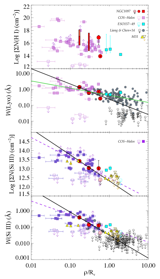
Figure 13.— Same as Fig. 12, now with the addition of values from published datasets, and with the x-axis extended beyond $1R_{v}$. Data from COS-Halos are shown as light pink squares for H I (Tumlinson et al., 2013) and purple squares for Si III (Werk et al., 2013). The black lines in the bottom three panels show the power-law fits to the NGC 1097 data alone from Fig. 12; the dashed purple lines for Si III show the fits from Werk et al. (2013) [where the slopes were found to be $-0.84\pm 0.24$ and $-1.11\pm 0.29$ for $W$(Si III) and $N$(Si III), respectively]. The green line in the second panel represents a least-squares fit to the COS-Halos and LC14 data, ignoring their upper limits.

In Figure 13 the COS-Halos data are shown as light pink squares, while the Si III values are purple squares. The H I column densities and EWs show a large dispersion, and include a set of sensitive non-detections at very small impact parameters which Tumlinson et al suggested was due to the lack of a cool halo around early type galaxies. These non-absorbing galaxies are only a small fraction of the total sample, and the bulk of the absorbers show unity covering fractions out to the $\sim 0.6\>R_{v}$ limit of the survey. Our range of $N$(H I) values, and the inferred covering fraction, appears consistent with the COS-Halos sample.

For Si III lines, Werk et al fitted a power law to the distribution of $N$(Si III) and $W$(Si III) with $\rho/R_{v}$ (ignoring both upper and lower limits). These fits are reproduced in the bottom two panels of Figure 13; their fits to $N$(Si III) and $W$(Si III) are close to what we find for the four sightlines towards NGC 1097. They also calculated a covering fraction for Si III of $73^{+9}_{-14}$% over a radius of $0-160$ kpc for galaxies with stellar masses $\log M_{*}(M_{\odot})\geq 10.5$. This again is consistent with the 3/4 detections in the halo of NGC 1097 at similar radii and at the same stellar mass limit.

In Figure 14 we introduce the detections and limits for C II (orange points), Si II (green points) and SI IV (blue points) for the COS-Halos galaxies. With C II, Si II and Si IV detections towards only Q0244, and a possible C II detection towards Q0246 (which we include) comparisons with NGC 1097 are tenuous. We note simply that the strengths of the metals towards NGC 1097 are similar to the COS-Halos sample. They lie in regions where the covering fraction of the metals in the COS-Halos sample are less than unity, and our non-detections are compatible with those low values.

8.1.2 Comparison to ESO 157-49

Three background probes were used by Keeney et al. (2013) to probe the edge-on galaxy ESO 157$-$149, a much less luminous ($L/L^{*}=0.12$) and weaker star-forming galaxy ($0.2-1.1$ $M_{\odot}$ yr^-1) than NGC 1097. We assume a viral mass of $\log M(M_{\odot})=10.6$ for the galaxy (the lower limit set by Keeney et al.), which corresponds to $R_{v}=88$ kpc. This puts their sightlines at impact parameters of $\rho/R_{v}\simeq 0.9,1.1$, and 2.0, distances larger than those probed for NGC 1097. We adopt the sum of the 3 $N$(H I) components towards the outermost sightline, HE 0435$-$5304, to be $\log N($H I) = $14.22\pm 0.11$ and calculate the total EW by reconstructing the line profile from their Voigt profile fits, $W$(Ly$\alpha$) = 0.63 Å. The Ly$\alpha$ lines towards the inner 2 sightlines are of similar strength to the inner two sightlines towards NGC 1097, and Keeney et al. had the same problem in determining $N$(H I) as we have had, with moderately strong $W$(Ly$\alpha$) yielding ambiguous column densities. Figure 13 shows these points compared to the NGC 1097 values; although the errors are large, $N$(H I) (filled cyan squares) appears to continue to decline with $\rho/R_{v}$ beyond 0.9$R_{v}$. Si III is detected towards the inner two ESO 157$-$49 sightlines, beyond the last limit from NGC 1097. No C II or Si II is detected towards any of the sightlines (open cyan squares) but Si IV is seen at distances beyond where the COS-Halos or the NGC 1097 data probe.

With the absorbers at either side of the major axis of the edge-on galaxy both having negative velocities relative to the galaxy, Keeney et al. concluded that the absorption (at least for one of the sightlines) was unlikely to be associated with any galaxy rotation, and that it was more likely to have arisen in material once ejected from the galaxy. This interpretation is clearly quite different from the ones discussed in §7 designed to account for the absorption towards NGC 1097.

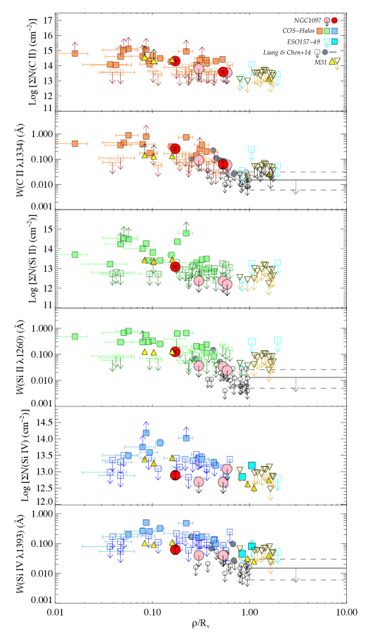
Figure 14.— Distribution of total column densities summed over all components, and equivalents widths, for C II, Si II and Si IV, as a function of impact parameter normalized by virial radius. Our data towards NGC 1097 are shown as red circles for detections, and pink circles for upper limits. Several other datasets are included for comparison, and their origin is shown in the legend top right of the first panel. Unfilled symbols represent upper limits, while lower limits (usually from mildly saturated lines) are indicated as filled symbols with the appropriate upward pointing arrow. Liang & Chen’s data contain a large number of EW upper limits beyond $1R_{v}$, and to avoid confusion, we draw the median of those upper limits with a single solid grey line and indicate the range of their limits with two dashed grey lines. Individual upper limits at $<1R_{v}$ are still plotted. Errors in $\rho/R_{v}$ are shown for the COS-Halos data, but to avoid confusion, they are omitted for the rest of the data sets. In most cases, uncertainties in $R_{v}$ are similar.

8.1.3 Comparison to M31

M31 offers an interesting comparison with NGC 1097 in that M31 has a luminosity and halo mass close to that of NGC 1097 (van der Marel et al., 2012a, b). The one important difference is that M31 is interacting with another galaxy of comparable mass only 0.8 Mpc away, with the same halo mass and luminosity — namely the Milky Way; as discussed in §2.3, there are no galaxies as bright as NGC 1097 within $4-5$ Mpc. Although there are a large number of QSOs that can be found at interesting impact parameters behind M31, the low velocity of the galaxy makes it difficult to study in absorption (§1). Nevertheless, Rao et al. (2013) found no absorption beyond $0.2\>R_{v}$ along the major axis of the disk (assuming $R_{v}=300$ kpc for M31), but low-ionization absorption from 4 of 6 sightlines below $0.1\>R_{v}$. These data are hard to incorporate in this study because i) the low resolution of the COS G140L and G230L observations make it difficult to fully separate out absorption from the strong MW ISM absorption lines, ii) understanding the relationship between the velocities of the detected lines and the velocity of MS+HVC gas (if any) at the positions probed is beyond the scope of this paper; and iii) both the Ly$\alpha$ and Si III $\lambda 1206$ line which are integral to our study are not available in their low resolution data. For these reasons, these data are not plotted in Figures 13 and 14. Nevertheless, Rao et al. drew an important distinction in claiming that M31 is not a typical Mg II absorbing galaxy compared to higher-redshift samples.

On the other hand, Lehner et al. (2015) used COS G130M and G160M Archival data of 18 sightlines passing within $2R_{v}$ of M31. They distinguished a specific velocity range over which to measure absorption that they considered sufficient to avoid contamination of MW ISM absorption and the MS. These data are included in Figures 13 and 14 (shown as triangles). Lehner et al. did not provide EW measurements from their data, and so we estimate EWs directly from the column densities assuming the lines are optically thin. These represent lower limits to the true EWs because not only may some of the lines be mildly saturated, but also because the wings of the absorption profile are often lost in the blended MW ISM and the MS lines either side of the absorption from M31.

8.1.4 Comparison to Intermediate-Redshift Sample

Like the COS-Halos sample, the collation by Liang & Chen (2014) is of absorption along single sightlines through many galaxies. Nevertheless, the sample is useful in that the sightlines probe beyond the impact parameters of the COS-Halos galaxies, and that measurements of many species of metal lines, as well as Ly$\alpha$, are provided. This sample of galaxies (hereafter designated as LC14) has a median redshift of 0.02, and samples galaxies with stellar masses of $10^{7}-10^{11}\>M_{\odot}$. Their derivation of $R_{v}$ is the same as described above, so we use their tabulated values. Only EWs are given by Liang & Chen, and since these cannot be converted to column densities with any reliability, column densities are not plotted. In Figure 13 all the data for Ly$\alpha$ and Si III $\lambda 1206$ are included, but in Figure 14, most points at $\rho/R_{v}>1.0$ are only upper limits, and not sensitive enough to show any significant decline in EW above those radii. To avoid confusion with points from the other datasets, we show only the median EW limit at $\rho/R_{v}>1.0$ as a grey horizontal bar.

8.1.5 Is NGC 1097 a typical absorber?

Our fitting of a power-law to the data obtained for NGC 1097 shows that the evidence for a decline in H I and Si III column densities and EWs with $\rho/R_{v}$ — based only on the 4 sightlines — is weak. Tumlinson et al. reported no decline in $N$(H I) or $W$(Ly$\alpha$) with $\rho/R_{v}$ in the COS-Halos sample, which we see recreated in the top panel of Figure 12. However, Figure 13 shows that when we combine the COS-Halos results with the LC14 data it seems more plausible that Ly$\alpha$ and Si III decline with impact parameter, and indeed that NGC 1097 follows the same decline. If we exclude the upper limits in the COS-Halos and LC14 datasets, then a linear regression analysis of the two larger samples confirms a strong correlation with a high probability of being able to exclude the null hypothesis that there is no correlation. A least-squares fit to the $W$(Ly$\alpha$) data (shown as a green line in the second panel of Fig. 13) has $\log W^{*}=-0.37\pm 0.02$ Å, $\alpha=-0.45\pm 0.04$; but more importantly, the standard error in the regression, $s$ is 0.27 dex, while for NGC 1097, $s=0.21$ dex. A similar result is found for $W$(Si III). This standard error is the average distance that the observed values fall from the fitted line, and conventionally, 95% of all points should fall within 2$s$. The fact that the values of $s$ for NGC 1097 and the two samples of COS-Halos and LC14 are similar suggests that the overall variability or clumpiness within the halo of NGC 1097 is largely the same as the dispersion seen from the galaxies in the larger single-probe datasets.

Of course, while the Ly$\alpha$ and Si III absorption in the halo of NGC 1097 may have much the same characteristics as the other datasets, we only know this to be true for impact parameters $<0.6R_{v}$. Beyond $1R_{v}$, LC14 have shown that the number of non-detections of Ly$\alpha$ increases rapidly, i.e. the covering fraction declines to $\sim 60$% at an EW threshold of 0.05 Å (their Fig. 11). Keeney et al.’s observations of ESO 157$-$49 does not show such a decrease (and remains as flat as the values for NGC 1097 at smaller $\rho/R_{v}$). Whether this represents the way H I is distributed around all galaxies, or whether the detection/non-detection of Ly$\alpha$ points to some other property of a galaxy that influences the extent of H I around its CGM, is not clear. Observations of additional probes beyond $0.6R_{v}$ for NGC 1097 would help explain how the covering fraction really declines in a single halo at large radii.

We conclude that based on the absorbing column densities and EWs alone, NGC 1097 — and probably M31 and ESO 157$-$49 — are ‘typical’ absorbers compared to the COS-Halos and LC14 samples. This is curious, because the structures which have been suggested as origins of the absorbing gas (an isolated galaxy for NGC 1097, an interacting group for the MW-M31-MS system, and post-ejection products from ESO 157$-$49) are quite different. It may be that while galaxies do indeed possess definable CGMs which decline with radius, some absorption line properties —- in this case $N$ and EWs — are relatively insensitive to the structures that contain the baryons. For NGC 1097 we have also used kinematics to attempt to better understand the origin of absorbing gas, leveraging the use of multiple probes of a single galaxy to constrain a model (an approach that is far more ambiguous for single sightlines through single galaxies). Again, though, a similar consideration of the kinematics of the three sightlines towards ESO 157$-$49 suggest an origin quite different than that for NGC 1097, and it remains to be determined if either set of results is universal for galaxies.

9. Discussion

9.1. Likely Origin of the Absorbing Gas

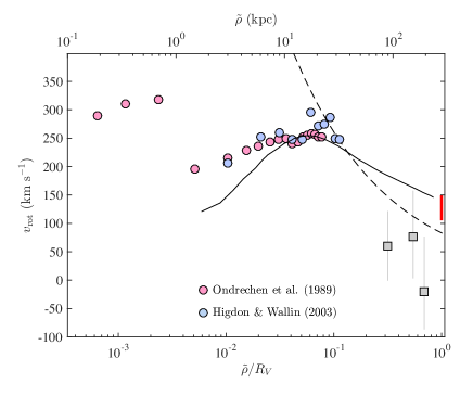
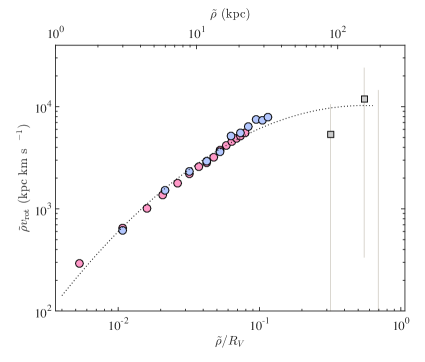
Figure 15.— Top: Rotation curve for NGC 1097’s inner disk from 21 cm data (pink and blue circles), compared to the absorbers in the CGM (grey squares) assuming that the absorbing gas is in the form of a disk and has the same inclination and position angle as the inner disk. All values are corrected for inclination effects. The sightline towards Q0244 leads to constraints on $v_{\rm{rot}}$ that are larger than the scale plotted on the y-axis, (because the sightline lies along the minor axis so has only a very small Doppler shift, and because the absorption is very broad) and so the sightline is excluded. The dashed line shows the expected $v_{\rm{rot}}$ if there were no dark matter beyond 25 kpc, and the black solid curve is a rescaled version of the Seljak (2002) galaxy-halo rotation curve. The vertical red line marks the expected virial speed for NGC 1097. If the absorbing gas really is in the configuration of a disk, the fact that $v_{\rm{rot}}$ is below the DM model expectations may imply that the gas is either infalling or that the disk is warped at large $\tilde{\rho}$. Bottom: Specific angular momentum of the gas. The dotted line shows a polynomial fit to the data.

We have shown in §7.1 that most of the absorption line profiles can be reproduced by a model in which gas is distributed in an extended rotating disk whose geometry matches those of the inner H I disk of NGC 1097. This implies that we are able to trace the rotation curve of the galaxy out to distances of $0.6R_{v}$. Figure 15 shows the 21 cm rotation curves obtained by Ondrechen et al. (1989) and Higdon & Wallin (2003) as a function $\tilde{\rho}/R_{v}$, in comparison to the Ly$\alpha$ lines towards the background QSOs. Figure 15 shows how velocities would decline for a Keplerian rotation; an extended disk model is only marginally consistent with being rotationally supported if there were no mass exterior to the inner H I disk (i.e. beyond $\sim 40$ kpc). Obviously, this is at odds with $\Lambda$CDM theory in general, and specifically, with the NGC 1097 system, where a large DM halo is required to produce the stellar streams (Higdon & Wallin, 2003; Amorisco et al., 2015). Instead, we are likely seeing absorption from an extended disk with a cool gaseous component, probably of low metallicity, falling into the inner disk of NGC 1097. Geometrically-thick quasi-disk gas distributions that are accreting on to a central object from large scales have been shown to occur naturally in simulations of structure formation (Kaufmann et al., 2006; Stewart et al., 2013; Danovich et al., 2015, e.g. their Fig. 13). There is evidence that such cold accretion inflows are now being detected at high redshift (Martin et al., 2015).

Figure 15 also shows that the specific angular momentum of the absorbing gas along the axis perpendicular to the inclined disk ($\tilde{\rho}\,v_{\rm{rot}}$) is consistent with that deduced from the 21 cm observations at the outer edges of NGC 1097’s disk. This implies that the accreting gas is infalling and does not lose angular momentum until it joins the inner halo at $\sim 0.3R_{v}$. This agrees with initial semi-analytic works on galaxy formation (e.g. Fall & Efstathiou, 1980) as well as the more recent simulations of Danovich et al. (2015) (see their Fig. 20) that explain the origin of angular momentum of galaxies by the deposition of gas from cold inflowing streams.

Our interpretation suggests that the spin parameter of the extended inclined disk (Dutton & van den Bosch, 2012, and refs. therein) is $\lambda_{\rm{extended-disk}}\simeq 0.15(\tilde{\rho}/100\>{\rm kpc})(v_{\rm{rot}}/70\>$km s^-1). This is $\sim 4$ times larger than the typical spins values of DM halos (Dutton & van den Bosch, 2012; Genel et al., 2015) and is consistent with the theoretical expectations for the spin of cold dense gas which originates from larger scales and accretes onto a halo.

Conversely, there is little obvious evidence to suggest that the absorption seen along the 4 QSO sightlines arises in outflowing gas from NGC 1097. Our attempts to replicate the kinematics of the absorption do a poor job when only outflowing gas is included, compared to the inflowing/rotating thick disk model. Nevertheless, adding an outflow to the thick disk model helps account for the A3 component towards Q0244. The primary constraint on such an outflow is that the opening angle must be large.

Moreover, galactic outflows are expected to have metallicities of order the solar value, while our investigations suggest that the absorbers might have metallicities less than this (Appendix C). The A3 component towards Q0244, again, is a possible exception, since we are unable to constrain its metallicity from photo-ionization considerations.

Finally, there is the issue of tidal debris around NGC 1097. As discussed in §2.2, NGC 1097 is interacting with an LMC-like galaxy (NGC 1097A), and has seen the passage of another, now destroyed, satellite galaxy which has given rise to the dog-leg stellar trail shown in Figure 1. It has been suggested that galaxy mergers and interactions are an effective way of distributing gas out to large distances and relative velocities from galaxies, and that complex, multi-component absorption line systems found in QSO spectra could be probing such debris (Bowen et al., 1994; Keeney et al., 2011; Rosenberg et al., 2014; Fox et al., 2014). The three outer QSO sightlines towards NGC 1097 show no obvious evidence for complex multicomponent structures spanning many hundreds of  km s^-1, which we might use to argue for the presence of tidal debris. The sightline towards Q0244, however, lies only $\simeq\>$15 kpc from Knot-A (at least, in projection), and only $\approx 10$ kpc from the limit of the trail discernable on the image. Components A1$-$A3 span only 157 km s^-1, but if the very weak positive-velocity Ly$\alpha$ components (A4 and A5) are included, the absorption covers at least 260 km s^-1. Indeed, the spread in velocity from components arising in tidal debris will depend strongly on the orientation of the debris structure. Structures that are roughly confined to a plane that is parallel to our sightline will show components that have velocities determined only by internal random motions rather than the bulk flow. Hence complex absorption lines may not be a necessary signature for tidal debris, particularly for minor mergers, where the disk of the more massive galaxy might be less perturbed.

Higdon & Wallin (2003) found no H I associated with the streams to a limit of 0.06 $M_{\odot}$ pc^-2 or $8\times 10^{18}$ cm^-2; at the position of the right-angle of the dog-leg trail, they set a limit of 0.021 $M_{\odot}$ pc^-2 or $3\times 10^{18}$ cm^-2 in a 4 arcsec aperture. [This is consistent with the value of $N$(H I) found towards Q0244.] Higdon & Wallin’s $N$-body simulations suggest that X-shaped tidal tails develop only after a second or third pass of the accreting galaxy through the host ($1.7-3.8$ Gyr from the first collision), and that the dwarf’s ISM will have been destroyed by ram pressure from the disk. In that case, there may be no remnants of cool gas associated with the dwarf or its interaction with the host galaxy. Our absorption line detections towards all four QSO sightlines, however, are sensitive to the much lower column densities that may arise in more highly ionized gas, and it remains possible that the absorption we see is related to the fate of the gas from the cannibalism of the dwarf galaxy.

We have seen in §7.1.2 that while a rotating, infalling disk can explain most of the kinematics of the absorption lines from NGC 1097, an additional model component of an conic outflow is needed to explain the A3 component to the absorption. It is possible that instead, this component — and the weak A4 and A5 Ly$\alpha$ lines — come from tidal debris associated with the stellar trails. This may help explain the difficulty in finding suitable solutions for photoionized gas in §C.1.2 for A3. The models of the debris constructed by Higdon & Wallin (their Fig. 13) show that stellar material ought to be distributed out to the sightlines of Q0244 and S393Z082, but, as expected, the covering fraction would probably depend quite strongly on the galaxy’s orientation to the line of sight. Modelling the evolution of gas associated with tidal mergers is beyond the scope of this paper. While the kinematics of the gas and the arguments made above show consistency with the models described, it is worth emphasizing that with only 4 sightlines, the correspondence could be fortuitous.

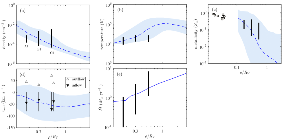
Figure 16.— Comparison between the results for the absorbers towards NGC 1097 and those predicted by the simulations of cold-mode gas accretion at $z=0$ made by van de Voort & Schaye (2012). The dashed blue lines mark the median of the property from their simulations, while the blue shaded regions mark the 16th to 84th percentiles around the median. Triangles mark upper or lower limits, while vertical bars mark the range of values, found from our analysis of the absorbers. The simulations calculate distances in real (3D) space, while we only probe projected impact parameters $\rho$; as shown in previous plots, however, $\rho$ and the de-projected values $\tilde{\rho}$ are similar for all but the outermost sightline, and we plot our data in terms of $\rho/R_{v}$. Panels (a) to (e) show the gas density, temperature, metallicity, inflow velocity and mass accretion rate assuming azimuthal symmetry in the plane of the disk. In panel (c) we plot inner disk metallicities of NGC 1097 (grey circles) taken from Moustakas et al. (2010) [using the normalization from Pilyugin & Thuan (2005)]. For the mass accretion rates in panel (e), van de Voort & Schaye do not quote estimates in the scatter of $\dot{M}$, so no blue shaded region is drawn. In panel (d) two sets of limits exist, either for inflowing or outflowing gas, while the vertical bars indicate the allowed inflow velocity range based on the rotating-inflowing disk model (§7.1.2). Overall, there is good agreement between the absorber properties deduced in this paper and these particular simulations.

9.2. Comparisons with simulations

As argued above, there are good reasons to believe that most of the absorbing gas we see in the CGM of NGC 1097 comes from material that is being accreted onto the galaxy from the outskirts of the halo. We conclude by comparing our data with one further set of simulations that evolve galactic structures down to $z=0$, those of van de Voort & Schaye (2012). Their calculations include radiative cooling, sub-grid star-formation and feedback prescriptions. Approximately 500 simulated halos are used to quantify the statistical properties of the halo gas. Conveniently, their results include a halo mass that is consistent with that of NGC 1097. Two ‘modes’ of gaseous structures are identified, a “cold-mode” component in the form of cool $<10^{5.5}$ K gas filaments, and a “hot-mode” component which contains a volume-filling gas component. Our data imply gas temperatures of $<10^{5}$ K, and so would be related to the cold-mode structures in the halo.

Figure 16 compares the results from the simulations with our analyses of the absorption systems. We find good agreement with many of the variables recorded in the simulations as they vary with $\rho/R_{v}$: the surface density profile is consistent with the model within the (non-negligible) uncertainties; the deduced gas temperatures coincide with the simulated values; and the absorbing gas metallicities also show good correspondence with the model.

The comparison between gas kinematics is shown on the bottom panel of the first column of Figure 16. It is impossible to distinguish an outflow that is launched away from us from the more distant side of a disk, from an infall of gas towards the side of a disk nearest to us. If we assume that the absorbers are falling towards the center of NGC 1097, then the absorption velocities are consistent with values in the simulation. We note however, that we only measure line-of-sight velocities, with a radial velocity component being potentially larger.

We can crudely estimate the mass infall rate from our data as a function of galactocentric radius, by assuming azimuthal symmetry: $\dot{M}(\tilde{\rho})\simeq\pi\tilde{\rho}^{2}N$(H) $(\tilde{\rho})(v_{\rm{rad}}/\tilde{\rho})$ . If $v_{\rm{rad}}$ is independent of $\tilde{\rho}$, we find $\dot{M}(\tilde{\rho})$ rises monotonically with $\tilde{\rho}$, as predicted in the simulations. Specifically, if we take a fiducial value of $v_{\rm{rad}}=70$ km s^-1, there is qualitative agreement between a mass infall rate of $\simeq 1M_{\odot}$ yr^-1 at small $\tilde{\rho}/R_{v}$ and the current star-formation rate, despite the $\gtrsim 1$ Gy dynamical timescales implied.

Figure 16 suggests good agreement between theoretical simulations and the absorption line data for NGC 1097. Intriguingly, van de Voort & Schaye noted that in their simulations, the probability of detecting these cold streams was low. Similarly, Goerdt et al. (2012, their Fig. 4) calculated a covering fraction of only $\sim 20$% for cool gas within $1R_{v}$ at $z=1.4$, with the value dropping with time. In the case of NGC 1097, and despite the small numbers of sightlines used, the covering fraction at $\log N$(H I)$\gtrsim 14$ is of order unity out to $\simeq 0.6R_{v}$. While it is possible that NGC 1097 may be unique in some way, there are no clear indications from the absorption line data that this is so. In fact, in §8.1.5, we argued that NGC 1097 was a ’typical’ absorber, in comparison to the ensemble of higher-redshift absorbers. If our results are not entirely due to a fortuitous combination of sightlines, then the apparent discrepancy could be related to problems with the simulations, a topic that is beyond the scope of this paper.

10. Summary

In this paper, we have observed 4 QSO whose sightlines pass through the halo of NGC 1097: Q0244$-$303 (referred to as Q0244 in the text), 2dFGRS S393Z082 (S393Z082), Q0246$-$308 (Q0246) and HE 0241$-$3043 (HE0241). These sightlines lie at impact parameters of 48, 84, 150, and 165 kpc, or $\approx 0.2,0.3,0.5$ and 0.6 times the virial radius of the galaxy, which we take to be $R_{v}=280$ kpc. We can summarise our results as follows:

1. We detect Ly$\alpha$ absorption towards all four sightlines. The total equivalent widths range from $\simeq 0.3-1.4$ Å, but the column densities towards the inner two sightlines are difficult to determine due to saturation of the lines. Nevertheless, they all have $N$(H I)$\>\geq 14.0$, which implies that the cross-section of NGC 1097 is unity out to 165 kpc ($0.6\>R_{v}$) at that limit. Si III $\lambda 1206$ is detected towards the 3 inner sightlines, with $W=0.13-0.39$ Å, all lines having $\log N$(Si III)$>13.0$, again suggesting a covering fraction of unity at 150 kpc ($0.5R_{v}$) at this column density.

2. The strongest Ly$\alpha$ absorption, and the one that shows the most metal lines (including C II, Si II, Si III and Si IV lines) occurs along the sightline to the inner-most sightline, Q0244$-$303 at 48 kpc ($0.2R_{v}$), and is comprised of a minimum of 2 components. A lower limit for the integrated column density of $\log N$(H I)$\>\geq\>15.7$ is robust, but the upper limit depends on whether a third component also exists, which is defined by the presence of a single C II component and no other metal lines. For a 2 component model, we establish $\log N$(H I)$\>\leq 17.1$, but if a third component exist, we cannot rule out a column density as high as $\log N$(H I)$\lesssim 18.1$. It is therefore possible that the absorption along this sightline is equivalent to a higher redshift Lyman limit system. This may also be true for the second inner-most sightline, 2dFGRS S393Z082 ($\rho\simeq 0.3\>R_{v}$), because although the Ly$\alpha$ line appears to consist of a single component, a high-$N$(H I)/low-$b$ profile fit is indistinguishable from a low-$N$(H I)/high-$b$ solution.

3. As noted above, Si IV is detected only along the inner-most sightline, with $\log N$(Si IV)$=12.9$. Beyond this, Si IV is absent at a level of $\log N$(Si IV)$\simeq\>12.7-13.1$, implying a small covering fraction at these limits beyond 48 kpc ($0.2R_{v}$).

4. There is only marginal evidence that $N$(H I) and $N$(Si III) decline with galactocentric radius, and the distribution of gas is clearly inhomogeneous within the CGM. We have fitted a power-law to the decline in column density with impact parameter, and for $W$(Ly$\alpha$) and $\log N$(Si III), the errors in the fit show that there could be no anti-correlation at all. An anti-correlation in $W$(Si III) with $\rho$ appears more plausible. In all cases, the CGM appears clumpy with respect to any possible smooth decline with $\rho$, and we characterize the clumpiness to be more than $\sim 0.2$ dex for an assumed power-law decline of $W$ and $N$ with $\rho$ for both Ly$\alpha$ and Si III.

5. We have modeled the observed column densities and column density limits using CLOUDY, assuming that the gas is photoionized. There are considerable uncertainties in the results, either because $N$(H I) is not well known and the SED of NGC 1097 is difficult to account for — as in the case towards Q0244$-$303 — or because few metals are actually detected (as towards the outer sightlines). The simplest solutions suggest that the gas has metallicities that are sub-solar, if the gas is dust-free.

6. We have attempted to replicate the observed absorption lines using a suite of models for the CGM around NGC 1097, including gas that is rotating in a huge extended disk, inflowing from the IGM, or outflowing from the galaxy. None of the models replicate the observations exactly, but one that has a disk of gas rotating roughly planar to, but more slowly, than the inner disk observed from 21 cm data, and which also includes gas infalling from the IGM, recreates the data well. The models that provide the poorest predictions of the data are those dominated by conical or spherical outflows. The exception to this statement arises in modeling the absorption towards Q0244$-$303, where the most positive velocity component requires additional absorption either from a broad outflow, or from tidal debris.

7. While these models provide a plausible insight into how the CGM may be distributed around NGC 1097, it is also possible that some of the absorption could arise from ionized gas associated with the stellar streams that exist around the galaxy as a result of a multiple-bypass minor merger. Gas associated with a cannabalized dwarf galaxy may have been stripped during its encounter, but its remains may contribute to the observed absorption.

8. In comparison only to the column densities and equivalent widths observed from the CGMs of other galaxies obtained from recent COS surveys, the absorption from NGC 1097 seems typical. Given the variations in these quantities in the single halo of NGC 1097, however, it may be that column density and equivalent width measurements are not a particularly sensitive way to disentangle how the origin of CGMs depend on the properties of the host galaxies. Our data demonstrate the necessity to observe absorption lines from the nearest local galaxies where the CGM can be defined a priori from multiple techniques, and that multiple probes of single galaxy CGMs is now a priority.

Table 3Equivalent widths and column densities towards v20, Q0244

	$v$	$\Delta v$	$\sigma(v)$	$W^{b}$	$b^{b}$	$\sigma(b)_{T}$
IDa	(km s-1)	(km s-1)	(km s-1)	(Å)	(km s-1)	(km s-1)	$\log(N)$	$\sigma(N)_{T}$
(1)	(2)	(3)	(4)	(5)	(6)	(7)	(8)	(9)
				H I Ly$\alpha$
A1	1227	$-44$	11	string${}^{-}|$	62.7	$-10.2,+8.7$	string15.57	$-0.23,+0.55$
A2	1261	$-10$	5	string1.316	$--$$--$$--$$--$$--$$--$ no unique fit $--$$--$$--$$--$$--$$--$
A3	1384	+113	2	string${}_{-}|$	18.9	$\pm 2.0$	string15.07	$-0.32,+0.24$
A4	1456	+185	2	string0.035	$\leq$9	…	$\geq$13.10	…
A5	1491	+220	3	string0.045	$\leq$9	…	$\geq$13.10	…
total [p]				string$1.385+0.035-0.058$			$\geq$15.69c	..
total [$N=90$]				string$1.365+0.095-0.109$				..
				C II $\lambda 1334$
A1	1227	$-44$	11	string0…	(52)	…	$<$13.9d	…
A2	1261	$-10$	5	string$0.062$	10.9	$-4.7$,+5.3	string13.62	$-0.08$,+0.12
A3	1384	+113	2	string$0.200$	24.4	$\pm 3.0$	string14.22	$\pm 0.03$
A4	1456	+185	2	$<$0.044	(9)	…	$<$13.46	…
A5	1491	+220	3	$<$0.046	(9)	…	$<$13.48	…
total [p]				string$0.261\pm 0.027$			string14.31	$\pm 0.03$
total [$N=60]$				string$0.266\pm 0.064$
				Si IIe
A1	1227	$-44$	11	$<$0.028	(52)	…	$<$12.24	…
A2	1261	$-10$	5	$<$0.028	(11)	…	$<$12.29	…
A3	1384	+113	2	string0.124	16.2	$\pm 2.4$	string13.09	$\pm 0.05$
A4	1456	+185	2	$<$0.028	(9)	…	$<$12.30	…
A5	1491	+220	3	$<$0.028	(9)	…	$<$12.30	…
total [p]				string$0.124\pm 0.013$			string13.09	$\pm 0.05$
total [$N=30$]				string$0.118\pm 0.020$
				Si III $\lambda 1206$
A1	1227	$-44$	11	string0.204	51.9	$-10.3,+11.4$	string13.08	$\pm 0.14$
A2	1261	$-10$	5	string0…	(11)	…	$<$12.2f0	…
A3	1384	+113	2	string0.183	24.9	$\pm 5.0$	string13.16	$\pm 0.07$
A4	1456	+185	2	$<$0.090	(9)	…	$<$13.01	…
A5	1491	+220	3	$<$0.090	(9)	…	$<$13.01	…
total [p]				string$0.387\pm 0.084$			string13.42	$\pm 0.03$
total [$N=60$]				string$0.380+0.134-0.162$
				Si IV $\lambda 1393^{g}$
A1	1227	$-44$	11	$<$0.034	(52)	…	$<$12.60	…
A2	1261	$-10$	5	$<$0.032	(11)	…	$<$12.62	…
A3	1384	+113	2	string0.063	30.2	$-9.2,+19.2$	string12.89	$\pm 0.13$
A4	1456	+185	2	$<$0.032	(9)	…	$<$12.64	…
A5	1491	+220	3	$<$0.032	(9)	…	$<$12.64	…
total [p]				string$0.063\pm 0.020$			string12.89	$\pm 0.13$
total [$N=30$]				string$0.058\pm 0.024$
				N V $\lambda 1238$
A1	1227	$-44$	11	$<$0.028	(52)	…	$<$13.13	…
A2	1261	$-10$	5	$<$0.028	(11)	…	$<$13.18	…
A3	1384	+113	2	$<$0.030	(30)	…	$<$13.17	…
A4	1456	+185	2	$<$0.030	(9)	…	$<$13.23	…
A5	1491	+220	3	$<$0.030	(9)	…	$<$13.23	…

Table 4Equivalent widths and column densities towards v40, S393Z082

	$v$	$\Delta v$	$\sigma(v)$	$W^{b}$	$b^{b}$	$\sigma(b)_{T}$
IDa	(km s-1)	(km s-1)	(km s-1)	(Å)	(km s-1)	(km s-1)	$\log(N)$	$\sigma(N)_{T}$
(1)	(2)	(3)	(4)	(5)	(6)	(7)	(8)	(9)
				H I Ly$\alpha$
B1	1240	$-31$	8	string$0.594\pm 0.036$	$19.1\leq b\leq 46.2$		string$17.60\geq\log N\geq 14.80$
total [$N=60$]				string$0.603+0.101-0.119$
				C II $\lambda 1334^{c}$
B1	1240	$-31$	8	$<$0.092	(22)	…	$<$13.80	…
				Si II $\lambda 1260$
B1	1240	$-31$	8	$<$0.036	(22)	…	$<$12.37	…
				Si III $\lambda 1206$
B1	1240	$-31$	8	string0.148$\pm 0.023$	22.2	$\pm 5.0$	string13.04	$\pm 0.08$
total [$N=30$]				string$0.140+0.054-0.060$
				Si IV $\lambda 1393$
B1	1240	$-31$	8	$<$0.040	(22)	…	$<$12.69	…
				N V $\lambda 1238$
B1	1240	$-31$	8	$<$0.048	(22)	…	$<$13.41	…

Table 5Equivalent widths and column densities towards v60, Q0246

	$v$	$\Delta v$	$\sigma(v)$	$W^{b}$	$b^{b}$	$\sigma(b)_{T}$
IDa	(km s-1)	(km s-1)	(km s-1)	(Å)	(km s-1)	(km s-1)	$\log(N)$	$\sigma(N)_{T}$
(1)	(2)	(3)	(4)	(5)	(6)	(7)	(8)	(9)
				H I Ly$\alpha$
C1	1269	$-20$	11	string0.269	34.7	$-2.7,+3.1$	string13.93	$-0.02,+0.03$
C2	1342	+71	3	string0.436	16.8	$-1.6,+4.7$	string16.89	$-1.39,+0.50$
C3	1488	+217	14	string0.070	28.7	$-8.6,+11.7$	string13.16	$-0.10,+0.13$
total [p]				string$0.707+0.056-0.047$			string16.89	$-1.14,+0.35$
total [$N=60$]				string$0.693\pm 0.055$
				C II $\lambda 1334$
C1	1269	$-20$	11	blended
C2	1342	+71	3	string0.063	14.5	$-5.7$,+6.6	string13.59	$-0.07,+0.09$
C3	1488	+217	14	$<$0.044	(29)	…	$<$13.37	…
total [p]				string$0.063\pm 0.019$			string13.59	$-0.07,+0.09$
				Si II $\lambda 1260$
C1	1269	$-20$	11	$<$0.036	(16)	…	$<$12.36	…
C2	1342	+71	3	$<$0.034	(17)	…	$<$12.36	…
C3	1488	+217	14	$<$0.040	(29)	…	$<$12.41	…
				Si III $\lambda 1206$
C1	1269	$-20$	11	string0.040	15.5	$-12.6,+13.5$	string12.33	$\pm 0.24$
C2	1342	+71	3	string0.085	9.3	$-3.8,+5.1$	string12.92	$-0.10,+0.56$
C3	1488	+217	14	$<$0.058	(29)	…	$<$12.49	…
total [p]				string$0.125\pm 0.029$			string13.02	$-0.07,+0.43$
total [$N=35$]				string$0.125+0.055-0.060$
				Si IV $\lambda 1393$
C1	1269	$-20$	11	$<$0.040	(16)	…	$<$12.68	…
C2	1342	+71	3	$<$0.040	(17)	…	$<$12.70	…
C3	1488	+217	14	$<$0.044	(29)	…	$<$12.73	…
				N V
C1	1269	$-20$	11	$<$0.030c	(16)	…	$<$13.47	…
C2	1342	+71	3	$<$0.030c	(17)	…	$<$13.49	…
C3	1488	+217	14	$<$0.038	(29)	…	$<$13.28	…

Table 6Equivalent widths and column densities towards v70, HE0241

	$v$	$\Delta v$	$\sigma(v)$	$W^{b}$	$b^{b}$	$\sigma(b)_{T}$
IDa	(km s-1)	(km s-1)	(km s-1)	(Å)	(km s-1)	(km s-1)	$\log(N)$	$\sigma(N)_{T}$
(1)	(2)	(3)	(4)	(5)	(6)	(7)	(8)	(9)
				H I Ly$\alpha$
D1	1219	$-52$	4	string0.087	16.0	$-6.6,+11.5$	string13.34	$-0.13,+0.22$
D2	1309	+38	2	string0.179	19.7	$\pm 4.3$	string13.82	$\pm 0.04$
total [p]				string$0.266\pm 0.050$			string13.95	$\pm 0.04$
				C II $\lambda 1334$
D1	1219	$-52$	4	$<$0.064	(16)	…	$<$13.59	…
D2	1309	+38	2	$<$0.060	(20)	…	$<$13.54	…
				Si II $\lambda 1260$
D1	1219	$-52$	4	$<$0.024	(16)	…	$<$12.19	…
D2	1309	+38	2	$<$0.024	(20)	…	$<$12.19	…
				Si III $\lambda 1206$
D1	1219	$-52$	4	$<$0.044	(16)	…	$<$12.39	…
D2	1309	+38	2	$<$0.046	(20)	…	$<$12.40	…
				Si IV $\lambda 1402^{c}$
D1	1219	$-52$	4	$<$0.048	(16)	…	$<$13.10	…
D2	1309	+38	2	$<$0.048	(20)	…	$<$13.08	…
				N V $\lambda 1238$
D1	1219	$-52$	4	$<$0.032	(16)	…	$<$13.22	…
D2	1309	+38	2	$<$0.032	(20)	…	$<$13.22	…

Appendix A Notes on Individual QSOs and GALEX Grism Observations

As noted in §3, we observed NGC 1097 as part of a GALEX Cycle 1 Guest Investigator program (Program 085) designed to obtain FUV grism spectra of UV-bright objects in nearby galaxy fields with the aim of discovering new extragalactic sources. In this Appendix we summarize these observations, as well as remark on the original discoveries of QSOs in the field of NGC 1097 which made the observations discussed in this paper possible.

Many of the largest angular-diameter galaxies in our original list of target fields were to be observed as part of the GALEX Nearby Galaxy Survey (NGS) (Gil de Paz et al., 2007). This made it possible to add grism observations as part of a GALEX SNAP program without needing to acquire long UV images beforehand. We observed NGC 1097 for 1786 sec on 26-Oct-2004 as part of this program, and a total of 117 grism spectra were extracted with good quality data in both FUV and NUV channels. Of these, 80% showed spectra with very irregular continua, decreasing to zero flux below 2000 Å, indicative of the spectral energy distribution of stars. Of the remaining objects with discernable FUV flux, nine already had published identifications, leaving three un-identified. These three unfortunately showed no discernable emission line features and could not be added to our list of potential targets. Hence for this field, we were not able to discover any new UV-bright AGN or QSOs near NGC 1097.

Even though our selection of QSOs behind nearby galaxies was constructed by first selecting UV-bright objects from GALEX data (§3), our eventual choice of targets relied on them having extant redshifts. While NED catalogs the majority of redshifts from all published redshift surveys, it turns out that for NGC 1097, much of the redshift information comes from surveys conducted three decades ago by Wolstencroft et al. (1983) and Arp et al. (1984). The apparent over-density of X-bright QSOs in the field, and a hypothesized alignment of some QSOs with the galaxy’s jets, made this field of particular interest to the latter author (Arp & Carosati, 2007; Arp, 1998). Several redshifts were measured for objects in the field of NGC 1097 as part of that research.

Q0244 was originally discovered as a $z=0.528$ X-ray source by Wolstencroft et al. (1983), (their “Q1097.2”); Arp et al. (1984) labelled this as “#27” in a follow-up paper. It was later recovered by the 2dF QSO Redshift Survey (Croom et al., 2004) as 2QZ J024649.8$-$300742, which confirmed the original detection of Mg II in emission, as well as several Balmer emission lines. We detected C IV emission at the correct wavelength in our GALEX grism data.

S393Z082 was detected as part of the 2dF Galaxy Redshift Survey (2dFGRS) (Colless et al., 2001), where broad, weak H$\beta$, H$\gamma$ and Mg II were clearly detected at $z=0.339$. Equally narrow and weak Ly$\alpha$ emission was also detected in our GALEX grism data at the expected wavelength.

Q0246  was discovered as an X-ray bright object by Arp et al. (1984), their “#35”. Their redshift of $z=1.09$ was determined unambiguously from optical data, and we detected strong and broad Ly$\alpha$ emission in our GALEX grism data.

HE0241 was discovered by Wisotzki et al. (2000) as part of the Hamburg/ESO survey for bright QSOs. We obtained no GALEX grism spectra for the QSO, since it lies just outside of the GALEX field centered on NGC 1097.

S394Z150 was identified as an AGN in the 2dFGRS with $z=0.131$, and we selected the target based on the cataloged redshift and measured FUV magnitude. No spectrum was supplied in the original grism catalog produced after the GALEX data were taken, but more recent GALEX Data Releases now provide a grism spectrum for the object. It shows the flux rising towards the FUV at levels predicted from the FUV magnitude, but is featureless. After obtaining the HST COS spectrum, it became apparent that the object is not extragalactic, and is likely to be a local White Dwarf star, based on the extremely strong damped Ly$\alpha$ absorption profile at $z=0$ and the weakness of any metal lines that would normally be expected from a sightline passing through the Milky Way. A retrospective examination of the optical spectrum from the 2dFGRS database shows that no emission or absorption lines were detected, making the original redshift measurement erroneous.

One final note: Wolstencroft et al. (1983) found a relatively bright X-ray QSO, J024645.60$-$300051.9 (their “Q1097.3”), with $z=1.00$. We recovered this QSO independently from our GALEX grism data, with Ly$\alpha$ emission clearly visible at the expected redshift. However, there is no FUV flux below a strong discontinuity at 1900 Å, which could be due to Lyman limit absorption at the redshift of the QSO itself. For this reason, this QSO was never a potential HST COS target.

Appendix B Notes on NGC 1097B

Figures 1 and 3 also show the position of NGC 1097B. This faint galaxy was reported by Higdon & Wallin (2003) to have a 21 cm velocity of 1015$\pm 11$ km s^-1. (The position of the galaxy appears to be mis-reported in their Table 1 but the position discussed in their text is only 13$"$ from the optical position of the 2dFGRS source.) It was also observed as part of the 2dF Galaxy Redshift Survey (2dFGRS), designated S393Z052 with $b_{J}=18.1$, and assigned a redshift of $z=0.0645$ ($\simeq 19,300$ km s^-1), but there is little evidence from the galaxy spectrum that this is correct. Indeed, although the spectrum is of low signal-to-noise (S/N), there is better evidence for a 4000 Å break and, perhaps, H$\alpha$ emission, close to the 1015 km s^-1 given by Higdon & Wallin (2003). The galaxy has an absolute magnitude $M(b_{J})=-12.5$ if at the redshift measured by Higdon & Wallin, reminiscent of the ultra-compact dwarf galaxies (UCDs) found by Phillipps et al. (2001) in the Fornax cluster, but NGC 1097B does not look as compact as those UCDs. It is possible that NGC 1097B constitues a third satellite of NGC 1097, although more accurate redshift information is obviously needed. There is no evidence for any absorption lines at the velocity of 1015 km s^-1 and there is no reason to suppose that the galaxy contributes directly to the detected absorption. It would, nevertheless, be of interest to determine if this is indeed another dwarf galaxy in the halo of NGC 1097.

Appendix C Notes on photoionization calculations for the absorption systems

All of the fits in Tables 3$-$6 are based on allowing the $b$-values of individual species to vary independently of one another. (The only parameter in common for all the lines are their fixed velocities.) An alternative approach might be to fit all the species demanding that the same Doppler parameter be used, an approach which would be acceptable if all the line widths were dominated by non-thermal processes. However, at certain temperatures, the widths of Ly$\alpha$ lines, and the widths of metal lines, can be dominated by different processes: it is well known that the width of a line is usually represented by summing, in quadrature, the width expected from thermal broadening by gas at a temperature $T$, $b_{\rm{therm}}$, with a width that describes a turbulent velocity $b_{\rm{turb}}$, such that the total width in km s^-1 is $b^{2}=b_{\rm{therm}}^{2}+b_{\rm{turb}}^{2}$, or for an ion of atomic mass $A$,

$$b^{2}=\frac{2k_{B}\,T}{A\,m_{p}}+b_{\rm{turb}}^{2},$$ (C1)

— assuming that the turbulent width can be adequately described by a Gaussian. (Here, as usual, $k_{B}$ is the Boltzmann constant and $m_{p}$ is the mass of the proton.) Hence if the kinetic temperature of H I is, e.g., $3000$ K, the thermal width of a Ly$\alpha$ line is $7$ km s^-1, while for metals such as, e.g., silicon, $b_{\rm{therm}}$ is only $\sim 1$ km s^-1. So while the thermal widths of the metal lines are largely unresolved at these temperatures in COS data, the thermal width of H I can be a significant fraction of the total line width as $T$ increases.

While $b_{\rm{therm}}$ and $b_{\rm{turb}}$ cannot be determined independently, we can make a series of fits to the H I and metal lines together, assuming a set of temperatures which fixes $b_{\rm{therm}}$ for each line, and which lets $b_{\rm{turb}}$ vary, while always constructing a total width from Equation C1 (which is used for fitting the observed profile). This yields a grid of column densities and values of $b_{\rm{turb}}$ for each $T$ (or $b_{\rm{therm}}$). Uncertainties on each model can be calculated using the same Monte-Carlo procedures described in §5.1. An example of the results from this multiple-$T$ fitting is shown in Figure 17 for both components of A1 and A3 towards Q0244. This method enables us to better understand the range of column densities — particularly $N$(H I) in this complicated system — that are likely causing the absorption. The only drawback is that we need to assume that the temperature of the two components (i.e. the $b_{\rm{therm}}$ values) are the same. This assumption need not be true, but so long as $b_{\rm{therm}}$ is not considerably different for the two components, the results remain largely valid.

Further, we can use these results to construct models for photoionized gas of density $n$ and metallicity $Z$ for each value of $T$. We do this using the CLOUDY software package (Ferland et al., 2013, version C08.01). The analysis assumes all abundances are relative to the total hydrogen density and are scaled to each other in a solar abundance pattern; the solar values for carbon and silicon come from Allende Prieto et al. (2002) and Holweger (2001), respectively. Unless otherwise stated in the sections that follow, the models are dust-free. We adopt a UV background based on the meta-galactic field of Haardt & Madau (1996, 2012, hereafter HM), but discuss the possible contribution from NGC 1097 itself when appropriate. The total hydrogen column density $N$(H) is obtained by scaling the solution to the measured $N$(H I) at that temperature, and the absorber scale-length $l=N$(H)$/n$ is deduced.

In the following sections we discuss the results of this analysis for the metal line components toward three of the sightlines. For HE0241, the two absorption components D1 and D2 (Table 6 and Fig. 9) are only detected in H I, and constraints on their physical properties are of little use. Hence no results are reported for these.

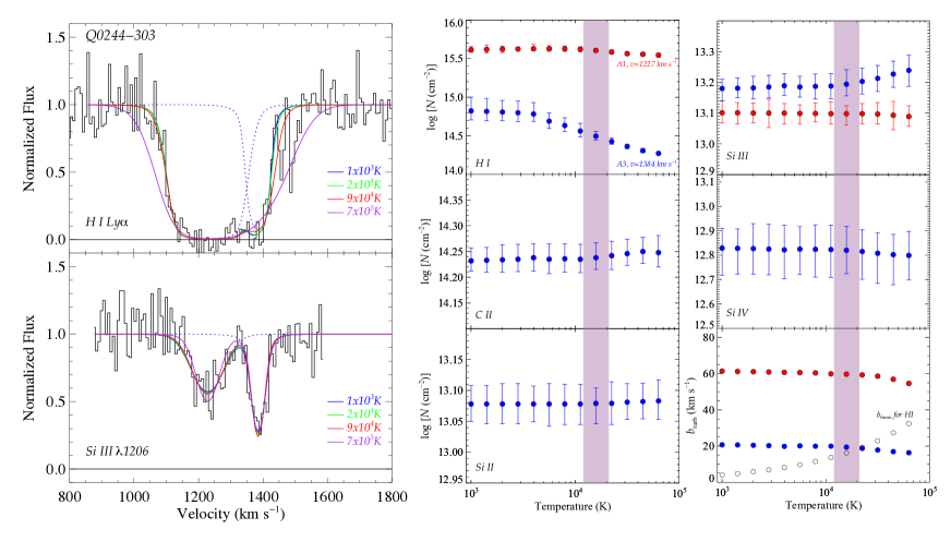
Figure 17.— Voigt-profile fits to the lines towards Q0244, assuming that the gas has a range of thermal temperatures. Left: Simultaneous fits to both the Ly$\alpha$ and Si III $\lambda 1206$ lines for a two component model when the $b$-value is determined by a combination of turbulent and thermal broadening, with the thermal component $b_{\rm{therm}}$ fixed by the four indicated temperatures $T$. (The thermal widths are by necessity assumed to be the same for both components.) Although only two species are shown here, the profiles are a result of simultaneous fits to all available lines. The dotted profiles indicate the individual components A1 and A3 that comprise the fit for $b_{\rm{therm}}$$=1\times 10^{3}$ K and are shown only to highlight the assumed 2-component nature of the line. Fits to the high-velocity weak Ly$\alpha$ lines (A4 & A5 in Fig. 5) are not shown here. The profiles demonstrate that the absorbing H I cannot be at temperatures $T\gtrsim 10^{5}$ K. Right: Variations in the column densities when $b_{\rm{therm}}$ — and hence $b_{\rm{turb}}$— changes with $T$. Red points are for component A1 and blue points are for A3. The metal column densities are largely insensitive to different temperatures, but $N$(H I) may change by $\sim 1$ dex for A3, making it difficult to reliably constrain the physical properties of the system. The purple-shaded regions mark the temperature range where the CLOUDY predictions discussed in §C.1 match the observed values. Bottom-right: the deduced turbulent velocities of the gas are shown for both A1 and A3, while the thermal speeds for H I are shown as black circles.

C.1. Absorption System Towards Q0244

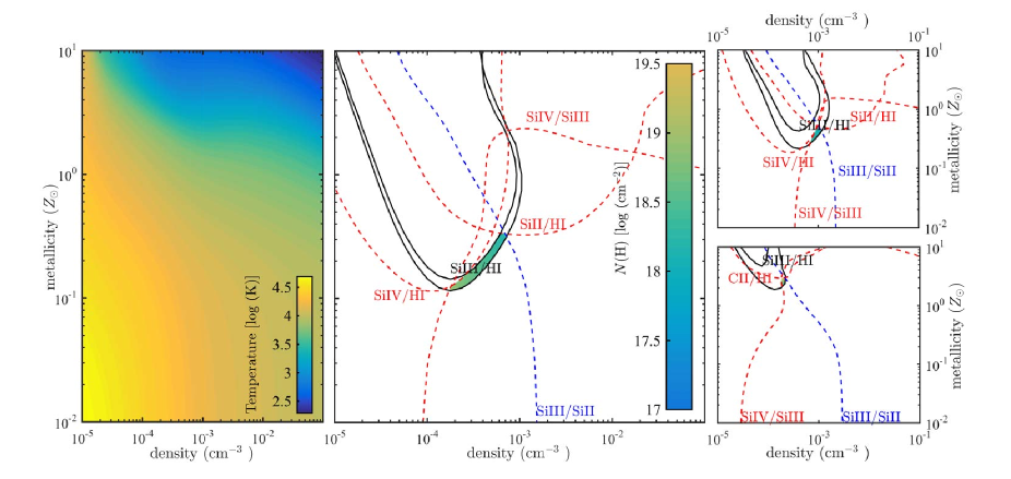
Figure 18.— Photoionization models for component A1 towards Q0244. Left: variations in temperature for different densities and metallicities, $T=T(n,Z)$, for photoionized, dust-free, optically thin gas exposed to the metagalactic background radiation field under non local thermodynamic equilibrium (non-LTE) conditions. Middle: the phase-space of $n$ and $Z$ allowed by the different column density ratios. Solid curves mark ratios for which measured column densities were available for both ions, plotted for $\pm 1\sigma$ variations as a result of the errors in the column densities. Dashed curves mark ion ratios for which only upper limits are available for one of the ions: upper limits to $n$ and $Z$ are marked in red while lower limits are shown in blue. The colored shaded region near the center marks the phase space that satisfies all the constraints, with the colors representing the total H column density (shown by the inset color-bar). For simplicity, only ion ratios that provide useful constraints are plotted. Right: the upper panel shows models for which the contribution of flux from NGC 1097 is included (see text) while the lower panel shows the effects of including Milky Way dust-to-metals mixtures (the latter yielding no solution). The colors of the lines in these panels are the same as those in the middle panel.

This system is the most complicated of the four studied. Our analysis is restricted to the A1 and A3 systems listed in Table 3 and labelled in Figure 5. Component A2 has no unique H I column density (and may not be real) while components A4 and A5 show only weak Ly$\alpha$ and no metal lines. Figure 17 shows that $N$(H I) for component A1 remains largely constant for all values of $b_{\rm{therm}}$, $\log N$(H I)$\>\simeq 15.6$. For component A3, $\log N$(H I)$\>=14.8$ for $T\sim 5\times 10^{3}$ K but decreases at higher temperatures. The metal-line column densities remain constant for all values of $b_{\rm{therm}}$. We should emphasize, however, that this apparently well-behaved change in $N$(H I) with temperature is strongly dependent on a likely over-simplified 2 component model: obviously, it is always possible that the entire Ly$\alpha$ complex could be made up of many more high-$N$(H I)/low-$b$ components that are blended together, and which we are unable to separate.

C.1.1 Photoionization models for Component A1

A single-phase solution (i.e. a single cloud with a uniform density) for this component which satisfies all the observational constraints is obtained for $n\lesssim 7\times 10^{-4}$ cm^-3 and $Z\lesssim 0.3\>Z_{\odot}$, which yields $\log N$(H)$\>\gtrsim\>18$ (Fig. 18). Taking the extreme values of this solution, the resulting length-scale is 0.5 kpc $\lesssim l\lesssim 10$ kpc, which implies that the gas occupies only a small fraction of the volume as $l/\rho<0.2$.

The contribution of NGC 1097 to the flux ionizing the absorbing gas along this sightline may not be negligible, given the relatively small impact parameter of Q0244. Assessing the galaxy’s contribution is difficult as the UV and X-ray flux that the absorbers see may depend on the galaxy’s inclination relative to where the clouds are, on their distance and orientation to star-forming regions in the disk, and on any contribution from the central AGN (all of which are highly uncertain). The spectral energy distribution (SED) of the UV background, which is dominated by galaxies at $z=0$, will likely have, to first order, a similar shape to that of NGC 1097, so the contribution from the galaxy can be accounted for by simply scaling-up the background flux level. In this case, a solution is obtained for the same ratio of photon-to-particle density, and the allowed density range scales with the flux level (by roughly +0.6 dex given the luminosity of NGC 1097).

Alternatively, we can at least qualitatively assess the effects of assuming that the SED below the He II edge is similar to that of the Milky Way (Fox et al., 2005), by using a flux below the He II edge that is twice as high as that given by the HM SED (and which includes a contribution from both quasars and galaxies); the results are shown in Figure 18, where a single-phase solution can only be found if the upper limit to the Si IV column density is under-estimated by 0.1 dex. The resulting model then has $n\sim 10^{-3}$ cm^-3, $Z\sim\>0.5\>Z_{\odot}$, $\log N$(H)$\>=18.0$ ($l\sim 0.3$ kpc), which implies slightly higher gas metallicities and slightly more compact absorbers.

We also consider the possibility that the elements might be depleted onto dust grains. Adopting any depletion patterns that are similar to the Milky Way is difficult, since these are known to differ widely for, e.g. disk and halo gas (e.g. Savage & Sembach, 1996). CLOUDY offers a compromise of using an average of values from both warm and cold gas, and we use these to see how our calculations might change with dust included. Ignoring any contribution to the UV flux from NGC 1097, using all the available column density ratios and limits, there is no single-phase solution. Only if we raise the column density upper limits by a factor of 2, and use $\pm 2\sigma$ intervals around the measured values, do we find a solution that has $Z\sim 3\>Z_{\odot}$ and $n\gtrsim 1\times 10^{-4}$ cm^-3. We consider it unlikely, however, that the errors and upper limits for the metal lines in A1 are so badly determined by our analysis, and we reject these values.

C.1.2 Photoionization models for Component A3

The analysis of this component yields no single-phase solution that can simultaneously account for all the observational constraints. The phase spaces for many line ratios are shown in Figure 19, and we see that none of the regions intersect. Considering the $N$(C II)/$N$(H I) ratio alone (for example), the phase space available is completely ruled out because the allowed area is completely outside the region plotted in Figure 19 (unless $Z>10\>Z_{\odot}$). As discussed in §5.3, $N$(H I) is poorly constrained for this component (although apparently less so than A1), which certainly adds to the difficulty in finding a suitable solution. Nevertheless, even allowing for a wide range of $N$(H I), there is no single-phase solution which accounts for all the metal line ratios alone (Fig. 19).

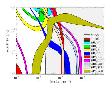
Figure 19.— Allowed $n,Z$ phase-space regions set by the different ion ratios for the A3 system towards Q0244. The inset legend shows how individual ion ratios are colored in the figure. No single-phase solution solution exists for the model because no region exists where all the colored regions intersect. The C II/H I ratio requires $Z>10\>Z_{\odot}$ and so is not shown at the scales used for this plot (i.e. $10^{-2}\>Z_{\odot}<Z<10\>Z_{\odot}$). Possible reasons for the poor agreement between model and observations include: a) that $N$(H I) is poorly determined, b) that the relative metal abundances are different from the solar values, and/or c) that multiple thermal phases are responsible for the absorption. If we consider only the silicon lines, a model with slightly super-solar abundances and densities of $\gtrsim 10^{-4}$ cm^-3 is implied.

This problem remains even if additional flux is added from NGC 1097, or if the absorbing gas is assumed to be depleted by dust like the Galactic ISM, and it persists even when pure collisional heating is considered instead of photoionization. The difficulties can be seen most acutely when considering low-ionization line ratios [in particular the $N$(Si II)/$N$(C II) ratio, which seems to be more shifted towards lower densities compared to the other line ratios], which suggests that the problem is not simply because we have searched for a single phase to explain all the line ratios simultaneously. For the particular case of $N$(Si II)/$N$(C II), if carbon is under-abundant by a factor of $\sim 3$ compared to the solar value, then the phase-space traced by this ratio is in better agreement with those of other metal-line column density ratios.

We can further attempt to constrain the physical conditions of the absorber by narrowly focussing on only the silicon lines, for which three ionization levels are observed: the gas density is then restricted by $N$(Si IV)/$N$(Si II) to be $10^{-4}$ cm${}^{-3}\lesssim n\lesssim 10^{-3}$ cm^-3 over nearly three decades in metallicity. Constraints for all silicon column density ratios yield a single-phase solution at $2\times 10^{-4}$ cm${}^{-3}<n<3\times 10^{-4}$ cm^-3 with $1.4\>Z_{\odot}<Z<3\>Z_{\odot}$. The total hydrogen column density depends on the uncertain $N$(H I), but is in the range $17.3<\log N$(H)$\><19.5$, which gives a scale-length $l\sim 0.2-50$ kpc.

In conclusion, the physical parameters of the A3 absorbing cloud remain far from clear. It is possible, for example, that the gas is not in equilibrium. In that case, a more detailed treatment of this system would require additional data.

C.2. Absorption System Towards S393Z082

This sightline shows a single system B1 (Table 4 and Fig. 6), and the results of our analysis is shown in Figure 20 (left panel). A solution is obtained within a range of $\pm 0.5$ dex around values centered at $n\sim 3\times 10^{-4}$ cm^-3, $Z\sim 0.1\>Z_{\odot}$, and $\log N$(H)$\>\lesssim 19$. This gives $l\sim 10$ kpc ($l/\rho\sim 0.1$) with deviations of up to $\pm 1$ dex of that value. At $\rho=84$ kpc, the contribution of any flux from NGC 1097 is smaller than it is for Q0244 (see above), which itself led to only small changes in metallicity and density for plausible changes in the SED. Assuming a Galactic-like ISM gas-to-dust mixture results in a solution with similar densities and total column densities, but with a metallicity increased to $\sim 0.5\>Z_{\odot}$.

C.3. Absorption System Towards Q0246

This sightline shows two closely blended components C1 and C2 (Table 5 and Fig. 8), and a third more kinematically distinct component C3. Only C2 shows metal line absorption, so we only discuss our results for that component.

The solutions we obtain for this system depends on whether the detection of the C II line is real (§5.5). Without including this line, we obtain a solution with $5\times 10^{-5}$ cm^-3 $<n<3\times 10^{-3}$ cm^-3 and $0.02\>Z_{\odot}<Z<0.2\>Z_{\odot}$ (Fig. 20, right panel), and a total column density in the range $3\times 10^{18}$ cm^-2$<N$(H)$\><3\times 10^{19}$ cm^-2, implying $0.3$ kpc $<l<300$ kpc. When including the ISM-like gas-to-dust patterns used in CLOUDY, the gas is found to have a similar density range, but with $0.2\>Z_{\odot}<Z<0.6\>Z_{\odot}$, and $\log N$(H)$\>\gtrsim 19.0$. As discussed above, there is a wide variation in the depletion patterns that exist in the Galactic ISM: our analysis shows merely that for depletions that are at least similar to the Galaxy, the deduced metallicity still appears to be sub-solar.

If we assume that the C II line is real, then a single phase solution is only found when the confidence levels are increased to 3$\sigma$ for C II. The allowed region in shown in magenta in Fig. 20. The deduced metallicity changes little, but the density is confined to a much smaller range.

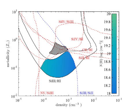
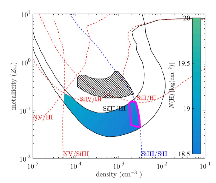
Figure 20.— Allowed phase-space for the absorption system B1 towards S393Z082 (left) and C2 towards Q0246 (right). (See Fig. 18 for details.) The hatched surfaces correspond to the allowed phase space when dust is included (see text).

References

- Allende Prieto et al. (2002) Allende Prieto, C., Lambert, D. L., & Asplund, M. 2002, ApJ, 573, L137
- Amorisco et al. (2015) Amorisco, N. C., Martinez-Delgado, D., & Schedler, J. 2015, ArXiv e-prints
- Arp (1976) Arp, H. 1976, ApJ, 207, L147
- Arp (1998) —. 1998, Seeing Red, p43 (Apeiron, Canada)
- Arp & Carosati (2007) Arp, H. & Carosati, D. 2007, ArXiv:0706.0143
- Arp et al. (1984) Arp, H., Wolstencroft, R. D., & He, X. T. 1984, ApJ, 285, 44
- Barth et al. (1995) Barth, A. J., Ho, L. C., Filippenko, A. V., & Sargent, W. L. 1995, AJ, 110, 1009
- Bechtold et al. (1994) Bechtold, J., Crotts, A. P. S., Duncan, R. C., & Fang, Y. 1994, ApJ, 437, L83
- Behroozi et al. (2013) Behroozi, P. S., Wechsler, R. H., & Conroy, C. 2013, ApJ, 770, 57
- Bessiere et al. (2012) Bessiere, P. S., Tadhunter, C. N., Ramos Almeida, C., & Villar Martín, M. 2012, MNRAS, 426, 276
- Bordoloi et al. (2014a) Bordoloi, R., et al. 2014a, ApJ, 794, 130
- Bordoloi et al. (2014b) Bordoloi, R., et al. 2014b, ApJ, 796, 136
- Borthakur et al. (2013) Borthakur, S., Heckman, T., Strickland, D., Wild, V., & Schiminovich, D. 2013, ApJ, 768, 18
- Borthakur et al. (2015) Borthakur, S., et al. 2015, ApJ, 813, 46
- Bowen et al. (2008) Bowen, D. V., et al. 2008, ApJS, 176, 59
- Bowen et al. (1994) Bowen, D. V., Roth, K. C., Blades, J. C., & Meyer, D. M. 1994, ApJ, 420, L71
- Bowen et al. (1997) Bowen, D. V., Tolstoy, E., Ferrara, A., Blades, J. C., & Brinks, E. 1997, ApJ, 478, 530
- Braun & Thilker (2004) Braun, R. & Thilker, D. A. 2004, A&A, 417, 421
- Burchett et al. (2016) Burchett, J. N., Tripp, T. M., Bordoloi, R., Werk, J. K., Prochaska, J. X., Tumlinson, J., Willmer, C. N. A., O’Meara, J., & Katz, N. 2016, ArXiv e-prints
- Burchett et al. (2015) Burchett, J. N., Tripp, T. M., Prochaska, J. X., Werk, J. K., Tumlinson, J., O’Meara, J. M., Bordoloi, R., Katz, N., & Willmer, C. N. A. 2015, ApJ, 815, 91
- Calzetti et al. (2010) Calzetti, D., et al. 2010, ApJ, 714, 1256
- Cen (2014) Cen, R. 2014, ApJ, 789, L21
- Chen et al. (2014) Chen, H.-W., Gauthier, J.-R., Sharon, K., Johnson, S. D., Nair, P., & Liang, C. J. 2014, MNRAS, 438, 1435
- Churchill et al. (2003) Churchill, C. W., Mellon, R. R., Charlton, J. C., & Vogt, S. S. 2003, ApJ, 593, 203
- Cioni et al. (2013) Cioni, M.-R. L., et al. 2013, A&A, 549, A29
- Colless et al. (2001) Colless, M., et al. 2001, MNRAS, 328, 1039
- Cooke et al. (2010) Cooke, R., Pettini, M., Steidel, C. C., King, L. J., Rudie, G. C., & Rakic, O. 2010, MNRAS, 409, 679
- Corbelli et al. (2010) Corbelli, E., Lorenzoni, S., Walterbos, R., Braun, R., & Thilker, D. 2010, A&A, 511, A89
- Croom et al. (2004) Croom, S. M., Smith, R. J., Boyle, B. J., Shanks, T., Miller, L., Outram, P. J., & Loaring, N. S. 2004, MNRAS, 349, 1397
- Cunnama et al. (2014) Cunnama, D., Andrianomena, S., Cress, C. M., Faltenbacher, A., Gibson, B. K., & Theuns, T. 2014, MNRAS
- Daddi et al. (2010) Daddi, E., Elbaz, D., Walter, F., Bournaud, F., Salmi, F., Carilli, C., Dannerbauer, H., Dickinson, M., Monaco, P., & Riechers, D. 2010, ApJ, 714, L118
- Danovich et al. (2015) Danovich, M., Dekel, A., Hahn, O., Ceverino, D., & Primack, J. 2015, MNRAS, 449, 2087
- de Vaucouleurs et al. (1991) de Vaucouleurs, G., de Vaucouleurs, A., Corwin, J. R., Buta, R. J., Paturel, G., & Fouque, P. 1991, in Third reference catalogue of Bright galaxies, New York : Springer-Verlag., 1
- Dinshaw et al. (1998) Dinshaw, N., Foltz, C. B., Impey, C. D., & Weymann, R. J. 1998, ApJ, 494, 567
- Dinshaw et al. (1997) Dinshaw, N., Weymann, R. J., Impey, C. D., Foltz, C. B., Morris, S. L., & Ake, T. 1997, ApJ, 491, 45
- D’Odorico et al. (1998) D’Odorico, V., Cristiani, S., D’Odorico, S., Fontana, A., Giallongo, E., & Shaver, P. 1998, A&A, 339, 678
- Doyle et al. (2005) Doyle, M. T., et al. 2005, MNRAS, 361, 34
- Dunn & Jerjen (2006) Dunn, L. P. & Jerjen, H. 2006, AJ, 132, 1384
- Dutton & van den Bosch (2012) Dutton, A. A. & van den Bosch, F. C. 2012, MNRAS, 421, 608
- Ellison et al. (2004) Ellison, S. L., Ibata, R., Pettini, M., Lewis, G. F., Aracil, B., Petitjean, P., & Srianand, R. 2004, A&A, 414, 79
- Fall & Efstathiou (1980) Fall, S. M. & Efstathiou, G. 1980, MNRAS, 193, 189
- Fang et al. (1996) Fang, Y., Duncan, R. C., Crotts, A. P. S., & Bechtold, J. 1996, ApJ, 462, 77
- Fathi et al. (2013) Fathi, K., et al. 2013, ApJ, 770, L27
- Ferguson & Sandage (1989) Ferguson, H. C. & Sandage, A. 1989, ApJ, 346, L53
- Ferland et al. (2013) Ferland, G. J., Porter, R. L., van Hoof, P. A. M., Williams, R. J. R., Abel, N. P., Lykins, M. L., Shaw, G., Henney, W. J., & Stancil, P. C. 2013, Rev. Mex. A&A, 49, 137
- Ford et al. (2014) Ford, A. B., Davé, R., Oppenheimer, B. D., Katz, N., Kollmeier, J. A., Thompson, R., & Weinberg, D. H. 2014, MNRAS, 444, 1260
- Fox et al. (2005) Fox, A. J., Savage, B. D., Wakker, B. P., Tripp, T. M., Sembach, K. R., & Bland-Hawthorn, J. 2005, ApJ, 630, 332
- Fox et al. (2014) Fox, A. J., et al. 2014, ApJ, 787, 147
- Galianni et al. (2010) Galianni, P., Patat, F., Higdon, J. L., Mieske, S., & Kroupa, P. 2010, A&A, 521, A20
- Gehrels (1986) Gehrels, N. 1986, ApJ, 303, 336
- Genel et al. (2015) Genel, S., Fall, S. M., Hernquist, L., Vogelsberger, M., Snyder, G. F., Rodriguez-Gomez, V., Sijacki, D., & Springel, V. 2015, ApJ, 804, L40
- Gil de Paz et al. (2007) Gil de Paz, A., et al. 2007, ApJS, 173, 185
- Goerdt et al. (2012) Goerdt, T., Dekel, A., Sternberg, A., Gnat, O., & Ceverino, D. 2012, MNRAS, 424, 2292
- Green et al. (2012) Green, J. C., et al. 2012, ApJ, 744, 60
- Greenhill et al. (2003) Greenhill, L. J., et al. 2003, ApJ, 590, 162
- Haardt & Madau (1996) Haardt, F. & Madau, P. 1996, ApJ, 461, 20
- Haardt & Madau (2012) —. 2012, ApJ, 746, 125
- Higdon & Wallin (2003) Higdon, J. L. & Wallin, J. F. 2003, ApJ, 585, 281
- Hobbs et al. (2013) Hobbs, A., Read, J., Power, C., & Cole, D. 2013, MNRAS, 434, 1849
- Holland et al. (2012) Holland, S. T., et al, & . 2012, Cosmic Origins Spectrograph Instrument Handbook, Tech. rep., Baltimore: STScI
- Holweger (2001) Holweger, H. 2001, in American Institute of Physics Conference Series, Vol. 598, Joint SOHO/ACE workshop ”Solar and Galactic Composition”, ed. R. F. Wimmer-Schweingruber, 23–30
- Hsieh et al. (2011) Hsieh, P.-Y., Matsushita, S., Liu, G., Ho, P. T. P., Oi, N., & Wu, Y.-L. 2011, ApJ, 736, 129
- Izumi et al. (2013) Izumi, T., et al. 2013, PASJ, 65, 100
- Kaufmann et al. (2006) Kaufmann, T., Mayer, L., Wadsley, J., Stadel, J., & Moore, B. 2006, MNRAS, 370, 1612
- Keeney et al. (2011) Keeney, B. A., Stocke, J. T., Danforth, C. W., & Carilli, C. L. 2011, AJ, 141, 66
- Keeney et al. (2013) Keeney, B. A., Stocke, J. T., Rosenberg, J. L., Danforth, C. W., Ryan-Weber, E. V., Shull, J. M., Savage, B. D., & Green, J. C. 2013, ApJ, 765, 27
- Kobayashi et al. (2002) Kobayashi, N., Terada, H., Goto, M., & Tokunaga, A. 2002, ApJ, 569, 676
- Kohno et al. (2003) Kohno, K., Ishizuki, S., Matsushita, S., Vila-Vilaró, B., & Kawabe, R. 2003, PASJ, 55, L1
- Koribalski et al. (2004) Koribalski, B. S., et al. 2004, AJ, 128, 16
- Kriss (2011) Kriss, G. 2011, Improved Medium Resolution Line Spread Functions for COS FUV Spectra, Tech. rep., STScI
- Lehner et al. (2015) Lehner, N., Howk, J. C., & Wakker, B. P. 2015, ApJ, 804, 79
- Lehner et al. (2014) Lehner, N., O’Meara, J. M., Fox, A. J., Howk, J. C., Prochaska, J. X., Burns, V., & Armstrong, A. A. 2014, ApJ, 788, 119
- Leroy et al. (2015) Leroy, A. K., et al. 2015, ApJ, 814, 83
- Liang & Chen (2014) Liang, C. J. & Chen, H.-W. 2014, MNRAS, 445, 2061
- Lopez et al. (2005) Lopez, S., Reimers, D., Gregg, M. D., Wisotzki, L., Wucknitz, O., & Guzman, A. 2005, ApJ, 626, 767
- Lopez et al. (1999) Lopez, S., Reimers, D., Rauch, M., Sargent, W. L. W., & Smette, A. 1999, ApJ, 513, 598
- Lorre (1978) Lorre, J. J. 1978, ApJ, 222, L99
- Madore et al. (1999) Madore, B. F., et al. 1999, ApJ, 515, 29
- Maller & Bullock (2004) Maller, A. H. & Bullock, J. S. 2004, MNRAS, 355, 694
- Martin et al. (2012) Martin, C. L., Shapley, A. E., Coil, A. L., Kornei, K. A., Bundy, K., Weiner, B. J., Noeske, K. G., & Schiminovich, D. 2012, ApJ, 760, 127
- Martin et al. (2015) Martin, D. C., Matuszewski, M., Morrissey, P., Neill, J. D., Moore, A., Cantalupo, S., Prochaska, J. X., & Chang, D. 2015, Nature, 524, 192
- McClure-Griffiths et al. (2009) McClure-Griffiths, N. M., et al. 2009, ApJS, 181, 398
- Meiring et al. (2013) Meiring, J. D., Tripp, T. M., Werk, J. K., Howk, J. C., Jenkins, E. B., Prochaska, J. X., Lehner, N., & Sembach, K. R. 2013, ApJ, 767, 49
- Mo & Miralda-Escude (1996) Mo, H. J. & Miralda-Escude, J. 1996, ApJ, 469, 589
- Monier et al. (1998) Monier, E. M., Turnshek, D. A., & Lupie, O. L. 1998, ApJ, 496, 177
- Monk et al. (1986) Monk, A. S., Penston, M. V., Pettini, M., & Blades, J. C. 1986, MNRAS, 222, 787
- Moustakas et al. (2010) Moustakas, J., Kennicutt, Jr., R. C., Tremonti, C. A., Dale, D. A., Smith, J.-D. T., & Calzetti, D. 2010, ApJS, 190, 233
- Muñoz-Mateos et al. (2011) Muñoz-Mateos, J. C., Boissier, S., Gil de Paz, A., Zamorano, J., Kennicutt, Jr., R. C., Moustakas, J., Prantzos, N., & Gallego, J. 2011, ApJ, 731, 10
- Murray et al. (2011) Murray, N., Ménard, B., & Thompson, T. A. 2011, ApJ, 735, 66
- Muzahid (2014) Muzahid, S. 2014, ApJ, 784, 5
- Norberg et al. (2002) Norberg, P., et al. 2002, MNRAS, 336, 907
- Norman et al. (1996) Norman, C. A., Bowen, D. V., Heckman, T., Blades, C., & Danly, L. 1996, ApJ, 472, 73
- Ondrechen et al. (1989) Ondrechen, M. P., van der Hulst, J. M., & Hummel, E. 1989, ApJ, 342, 39
- Petry et al. (1998) Petry, C. E., Impey, C. D., & Foltz, C. B. 1998, ApJ, 494, 60
- Phillipps et al. (2001) Phillipps, S., Drinkwater, M. J., Gregg, M. D., & Jones, J. B. 2001, ApJ, 560, 201
- Piñol-Ferrer et al. (2014) Piñol-Ferrer, N., Fathi, K., Carignan, C., Font, J., Hernandez, O., Karlsson, R., & van de Ven, G. 2014, MNRAS, 438, 971
- Pilyugin & Thuan (2005) Pilyugin, L. S. & Thuan, T. X. 2005, ApJ, 631, 231
- Prieto et al. (2005) Prieto, M. A., Maciejewski, W., & Reunanen, J. 2005, AJ, 130, 1472
- Putman et al. (2009) Putman, M. E., Peek, J. E. G., Muratov, A., Gnedin, O. Y., Hsu, W., Douglas, K. A., Heiles, C., Stanimirovic, S., Korpela, E. J., & Gibson, S. J. 2009, ApJ, 703, 1486
- Quillen et al. (1995) Quillen, A. C., Frogel, J. A., Kuchinski, L. E., & Terndrup, D. M. 1995, AJ, 110, 156
- Rao et al. (2013) Rao, S. M., Sardane, G., Turnshek, D. A., Thilker, D., Walterbos, R., Vanden Berk, D., & York, D. G. 2013, MNRAS, 432, 866
- Rauch et al. (2001) Rauch, M., Sargent, W. L. W., & Barlow, T. A. 2001, ApJ, 554, 823
- Rauch et al. (2002) Rauch, M., Sargent, W. L. W., Barlow, T. A., & Simcoe, R. A. 2002, ApJ, 576, 45
- Rogerson & Hall (2012) Rogerson, J. A. & Hall, P. B. 2012, MNRAS, 421, 971
- Rosenberg et al. (2014) Rosenberg, J. L., Haislmaier, K., Giroux, M. L., Keeney, B. A., & Schneider, S. E. 2014, ApJ, 790, 64
- Rubin et al. (2012) Rubin, K. H. R., Prochaska, J. X., Koo, D. C., & Phillips, A. C. 2012, ApJ, 747, L26
- Rubin et al. (2014) Rubin, K. H. R., Prochaska, J. X., Koo, D. C., Phillips, A. C., Martin, C. L., & Winstrom, L. O. 2014, ApJ, 794, 156
- Rupke & Veilleux (2013) Rupke, D. S. N. & Veilleux, S. 2013, ApJ, 768, 75
- Savage et al. (1990) Savage, B. D., Edgar, R. J., & Diplas, A. 1990, ApJ, 361, 107
- Savage et al. (2014) Savage, B. D., Kim, T.-S., Wakker, B. P., Keeney, B., Shull, J. M., Stocke, J. T., & Green, J. C. 2014, ApJS, 212, 8
- Savage & Sembach (1996) Savage, B. D. & Sembach, K. R. 1996, ARA&A, 34, 279
- Scannapieco & Brüggen (2015) Scannapieco, E. & Brüggen, M. 2015, ApJ, 805, 158
- Seljak (2002) Seljak, U. 2002, MNRAS, 334, 797
- Shull (2014) Shull, J. M. 2014, ApJ, 784, 142
- Skibba et al. (2011) Skibba, R. A., et al. 2011, ApJ, 738, 89
- Smette et al. (1995) Smette, A., Robertson, J. G., Shaver, P. A., Reimers, D., Wisotzki, L., & Koehler, T. 1995, A&AS, 113, 199
- Smette et al. (1992) Smette, A., Surdej, J., Shaver, P. A., Foltz, C. B., Chaffee, F. H., Weymann, R. J., Williams, R. E., & Magain, P. 1992, ApJ, 389, 39
- Sternberg et al. (2002) Sternberg, A., McKee, C. F., & Wolfire, M. G. 2002, ApJS, 143, 419
- Stewart et al. (2013) Stewart, K. R., Brooks, A. M., Bullock, J. S., Maller, A. H., Diemand, J., Wadsley, J., & Moustakas, L. A. 2013, ApJ, 769, 74
- Stinson et al. (2012) Stinson, G. S., et al. 2012, MNRAS, 425, 1270
- Stocke et al. (2013) Stocke, J. T., Keeney, B. A., Danforth, C. W., Shull, J. M., Froning, C. S., Green, J. C., Penton, S. V., & Savage, B. D. 2013, ApJ, 763, 148
- Thompson et al. (2005) Thompson, T. A., Quataert, E., & Murray, N. 2005, ApJ, 630, 167
- Toomre (1964) Toomre, A. 1964, ApJ, 139, 1217
- Tripp et al. (2011) Tripp, T. M., et al. 2011, Science, 334, 952
- Tripp et al. (2008) Tripp, T. M., Sembach, K. R., Bowen, D. V., Savage, B. D., Jenkins, E. B., Lehner, N., & Richter, P. 2008, ApJS, 177, 39
- Tripp & Song (2012) Tripp, T. M. & Song, L. 2012, ApJ, 746, 173
- Tully & Fisher (1977) Tully, R. B. & Fisher, J. R. 1977, A&A, 54, 661
- Tully et al. (2008) Tully, R. B., Shaya, E. J., Karachentsev, I. D., Courtois, H. M., Kocevski, D. D., Rizzi, L., & Peel, A. 2008, ApJ, 676, 184
- Tumlinson et al. (2013) Tumlinson, J., et al. 2013, ApJ, 777, 59
- van de Voort & Schaye (2012) van de Voort, F. & Schaye, J. 2012, MNRAS, 423, 2991
- van der Marel et al. (2012a) van der Marel, R. P., Besla, G., Cox, T. J., Sohn, S. T., & Anderson, J. 2012a, ApJ, 753, 9
- van der Marel et al. (2012b) van der Marel, R. P., Fardal, M., Besla, G., Beaton, R. L., Sohn, S. T., Anderson, J., Brown, T., & Guhathakurta, P. 2012b, ApJ, 753, 8
- Veilleux et al. (2005) Veilleux, S., Cecil, G., & Bland-Hawthorn, J. 2005, ARA&A, 43, 769
- Veilleux et al. (2001) Veilleux, S., Shopbell, P. L., & Miller, S. T. 2001, AJ, 121, 198
- Waugh et al. (2002) Waugh, M., et al. 2002, MNRAS, 337, 641
- Wehrle et al. (1997) Wehrle, A. E., Keel, W. C., & Jones, D. L. 1997, AJ, 114, 115
- Werk et al. (2013) Werk, J. K., Prochaska, J. X., Thom, C., Tumlinson, J., Tripp, T. M., O’Meara, J. M., & Peeples, M. S. 2013, ApJS, 204, 17
- Williams & Hodge (2001) Williams, B. F. & Hodge, P. W. 2001, ApJ, 559, 851
- Wisotzki et al. (2000) Wisotzki, L., Christlieb, N., Bade, N., Beckmann, V., Köhler, T., Vanelle, C., & Reimers, D. 2000, A&A, 358, 77
- Wolstencroft et al. (1983) Wolstencroft, R. D., Ku, W. H.-M., Arp, H. C., & Scarrott, S. M. 1983, MNRAS, 205, 67
- Wolstencroft & Zealey (1975) Wolstencroft, R. D. & Zealey, W. J. 1975, MNRAS, 173, 51P
- Zahedy et al. (2016) Zahedy, F. S., Chen, H.-W., Rauch, M., Wilson, M. L., & Zabludoff, A. 2016, MNRAS, 458, 2423
- Zuo et al. (1997) Zuo, L., Beaver, E. A., Burbidge, E. M., Cohen, R. D., Junkkarinen, V. T., & Lyons, R. W. 1997, ApJ, 477, 568